Wheat genotypes evaluated under North Eastern plains zone of the country for genotype x environment interaction analysis
Bạn đang xem bản rút gọn của tài liệu. Xem và tải ngay bản đầy đủ của tài liệu tại đây (475.45 KB, 14 trang )
Int.J.Curr.Microbiol.App.Sci (2020) 9(5): 1257-1270
International Journal of Current Microbiology and Applied Sciences
ISSN: 2319-7706 Volume 9 Number 5 (2020)
Journal homepage:
Original Research Article
/>
Wheat Genotypes Evaluated under North Eastern Plains Zone of the
Country for Genotype X Environment Interaction Analysis
Ajay Verma* and G. P. Singh
ICAR-Indian Institute of Wheat & Barley Research, Karnal 132001 Haryana, India
*Corresponding author
ABSTRACT
Keywords
AMMI analysis,
ASV, ASTAB, EV,
D, MASV, Biplot
graphs
Article Info
Accepted:
10 April 2020
Available Online:
10 May 2020
AMMI analysis observed highly significant values of environments, GxE interaction effects and genotypes effects for
both the years of study. Lower values of EV1 during (2016-17) ranked genotypes as (G6, G2, G8); D1 for (G6, G2,
G8); values of ASTAB1 for (G6, G2, G8) while SIPC1 for (G7, G1, G5) genotypes. EV2 measure pointed towards (G6,
G2, G9) as desirable, D2 for (G6, G2, G8), whereas as per SIPC2 were (G5, G7, G8) & ASTAB2 opted for (G6, G2,
G9). ASV and ASV1 recommended (G6, G2, G9) genotypes possessing stable performance as measures used 56.9% of
GxE interaction. Ranked values of EV3 preferred G2, G6, G8; SIPC3 pointed towards G5, G8, G1; D3 identified G2,
G6, G8 and ASTAB3 considered G2, G6, G8 wheat genotypes. Numerical values of D7 ranked G6, G2, G8; SIPC7
chosen G8, G1, G5. EV7 pointed towards G2, G6, G8 & ASTAB7 identified G9, G1, G4 as desirable over the studied
environments. Composite measure MASV selected G6, G2, G9 & MASV1 cited as G6, G2, G8 would be desirable.
Genotypes G8, G2 and G6 by Mean, GAI, HM, PRVG and MHPRVG measures would be of choice across environments
of study. Biplot analysis of studied measures exhibited three major clusters and most of the measures clubbed in first
cluster. Seven significant IPCA’s were used to calculate AMMI based measures during second year (2017-18) as
accounted more than 96.6%. Minimum values of EV1 ranked (G9, G6, G1), D1 pointed (G9, G6, G1) , ASTAB1 for
(G9, G6, G1) and for SIPC1 were (G7, G5, G10). EV2 pointed towards (G9, G1, G6) as desirable, for values of D2
genotypes were (G9, G1, G6) as per criterion of SIPC2 were (G7, G5, G10) & ASTAB2 favoured (G9, G1, G6). ASV
and ASV1 recommended (G9, G1, G6) as of stable performance. D7 expressed minimum values G9, G1, G6; SIPC7
observed G5, G9, G10, measure EV7 pointed towards G1, G5, G4. ASTAB7 identified G9, G1, G4 as desirable.
Composite measure MASV selected G9, G5, G1 and MASV1 as G9, G1, G5 for desirable performance. Genotypes G8
G9 by Mean, G7, G4 by GAI & HM, G4, G10 by PRVG and G7, G4 by MHPRVG measures based on yield of
genotypes across environments of study. Association analysis among AMMI measures and yield based analytic measures
by multivariate hierarchical Ward’s clustering approach grouped into four major clusters. Largest group I clubbed
measures as MASV1, ASV, MASV, D2, D3, D7, with EV2, EV3, SIPC5, SIPC7, EV7. Group II contains ASTAB1,
ASTAB2, ASTAB5, D1, D5, EV1, EV5, ASV1 whereas yield based measures exhibited close proximity and placed
close to each other as in separate group.
Introduction
Quite large number of statistical methods are
available for analysis of multi environment
trials, aimed to subdivide the complex GxE
interaction into simpler and more meaningful
responses of genotypes among studied
environments (Agahi et al., 2020). Multi
Environment trials of cereal crops had been
planned to have efficient estimation of main
and interaction effects (Bocianowski et al.,
2019). The procedures vary from univariate
parametric, non-parametric and multivariate
models. AMMI model ((Additive main effects
and multiplicative interaction), incorporates
both additive and multiplicative components
with aim to summarize the genotypeenvironment interaction (Guilly et al., 2017).
1257
Int.J.Curr.Microbiol.App.Sci (2020) 9(5): 1257-1270
Although, analysis of variance (ANOVA)
provided an interaction sum of squares that
would be difficult to interpret and the
prediction of yields in different environments
is not easy (Kamila et al., 2016). AMMI
separates the additive variance from the
multiplicative variance and then applies
principal component analysis (PCA) to the
interaction portion to a new set of coordinate
axes that explains in more detail the
interaction pattern (Tekdal & Kendal, 2018).
AMMI analysis has been shown to be
effective because it captures a large portion of
the GxE sum of squares, clearly separating
main and interaction effects that provide
researchers with different opportunities
(Gauch 2013; Tena et al., 2019). Prime
objectives of this study are (i) AMMI based
measures depend on utilization of significant
principal components (ii) explore the
association among AMMI along with yield
and adaptability measures.
Materials and Methods
North Eastern Plains Zone of India comprises
eastern Uttar Pradesh, Bihar, Jharkhand,
Assam and plains of West Bengal. Nine
advanced wheat genotypes twelve locations
and eleven genotypes at fifteen locations were
evaluated under field trials at of north eastern
plains zone during 2017-18 and 2018-19
cropping seasons respectively. Field trials
were conducted at research centers in
randomized complete block designs with
three replications.
Recommended agronomic practices were
followed to harvest good yield. Details of
genotype parentage along with environmental
conditions were reflected in tables 1 & 2 for
ready reference. AMMI first calculate
genotype and environment additive effect
using analysis of variance (ANOVA) and then
analyse residual from these model using
principal components analysis (PCA). AMMI
stability value (ASV) was initially proposed
by Purchase (1997) to quantify the stability
measure by considering relative weight of
IPCA1 and IPCA2 scores. In certain cases
where more than two IPCAs were significant,
ASV failed to encompass all the variability
explained by GEI. In order to overcome this
difficulty, Zali et al., (2012) attempted to
present a modified version ASV i.e., Modified
ASV which would cover all available IPCAs.
But in doing so, Zali et al., (2012) interpreted
the formula of ASV incorrectly compared to
the original formula of Purchase (1997). In
the present study the MASV of Zali et al.,
(2012) and a revised version of MASV (Ajay
et al., 2019) were compared with other
AMMI based measures. The description of
widely used measures based on AMMI
analysis was mentioned for completeness.
Zobel
1994
EV1
EVF
Sneller et al.,
1997
SIPC1
SIPCF
Purchase
1997
ASV
ASV = [
Annicchiarico
1997
D
D=
Rao and
Prabhakaran
2005
ASTAB
1258
Int.J.Curr.Microbiol.App.Sci (2020) 9(5): 1257-1270
Zali et al.,
2012
Zali et al.,
2012
Ajay et al.,
2019
ASV1
ASV1 = [
AMMI analysis was performed using
AMMISOFT version 1.0, available at
/>hughgauch/ and SAS software version 9.3. AMMI
based measures were compared with recent
analytic measures of adaptability calculated as
the relative performance of genetic values
(PRVG) and MHVG (Harmonic mean of
Genetic Values), based on the harmonic mean
of the genotypic values across different
environments.
Another harmonic mean based measure of the
relative performance of the genotypic values
(MHPRVG) for the simultaneous analysis of
stability, adaptability and yield (Resende &
Durate, 2007).
genotype across environments and n is
number of environments. Genotypes with
higher values of GAI are desirable
Results and Discussion
AMMI
analysis
provided
a
better
understanding of the GxE interaction through
analysis of variance, facilitated discriminating
environments and adaptability of the
genotypes to specific environments. Actually
AMMI fits a family of models with retaining
0, 1, 2, or more significant interaction
principal components (IPCs).
First year (2017-18)
AMMI analysis
PRVGij = VGij / VGi
MHVGi = Number of environments /
MHPRVGi.
= Number of environments /
VGij is the genotypic value of the i genotype,
in the j environment, expressed as a
proportion of the average in this environment.
Geometric
adaptability
index
(GAI)
(Mohammadi & Amri, 2008) was calculated
as
; in which 1, 2, 3, … m are
the mean yields of the first, second and mth
Model diagnosis is required to determine the
suitable AMMI model for a given dataset
while satisfying statistical and practical
considerations. FR-tests at the 0.01 level
diagnose AMMI6. Sums of squares for GxE
signal and noise were 85.47% and 14.53%
respectively of total GxE sum of squares.
Sum of Squares for GxE signal is 3.53 times
of genotypes main effects depicts narrow
adaptations are important for this dataset.
Even just IPC1 alone is 1.56 times the
genotypes main effects. Also note that GxE
noise is 0.60 times the genotypes main
1259
Int.J.Curr.Microbiol.App.Sci (2020) 9(5): 1257-1270
effects. Highly significant environments, GxE
interactions and genotypes effects were
depicted in table 3. Large magnitude of GxE
interactions for yield found in this
investigation are similar to those found in
other crops (Nowosad et al., 2018). AMMI
derived measures based on the use of
significant IPCA’s were calculated as EV1,
ASTAB1, SIPC1, D1 measures (only first
significant IPCA), while ASV, EV2,
ASTAB2, SIPC2, ASV1, D2 considered
IPCA1 & IPCA2, measures EV3, ASTAB3,
SIPC3 and D3 used three IPCAs, measures
EV5, ASTAB5, SIPC5 & D5 (based on five
IPCAs), and finally EV7, ASTAB7, SIPC7
and D7 measures utilized all significant
IPCAs.
Significant GxE interactions sum of squares
was further divided into seven significant
interaction principal component axes (IPCAs)
mentioned in table 3. Explained variation of
GxE interaction accounted by each of IPCA
exploited by defined measures, as type-1
AMMI based measures benefited 37.7%,
type-2 measures utilized 60.4%, type 3
measures used up to 73.8%, type 5 measures
benefited up to 92.6%, while type 7 measures
accounted for most of variation and utilized to
the extent of benefits 99.6% (Table 3).
This justifies the use of AMMI derived
measures based on the large numbers of
IPCAs results in the most usage of GxE
interaction variations (Mohammadi et al.,
2015; Kendal &Tekdal, 2016).
Lower and maximum values of EV1 ranked
genotypes as (G6, G2, G8) and (G7, G1)
whereas for D1 were (G6, G2, G8) and (G7,
G1) values of ASTAB1 for (G6, G2, G8) and
(G7, G1) and for SIPC1 were (G7, G1, G5) &
(G3, G4), of low yield performance (Tables 5
& 6). EV2 measure pointed towards (G6, G2,
G9) as desirable and (G1, G5) vice versa, D2
for genotypes (G6, G2, G8) & (G1, G3),
whereas as per SIPC2 were (G5, G7, G8) &
(G3, G4) and of ASTAB2 were (G6, G2, G9)
& (G1, G3). In recent studies, agronomic
concept of stability would be more preferred
instead of static concept of stability (Nowosad
et al., 2016). Using first two IPCAs in
stability analysis could benefits dynamic
concept of stability in identification of the
stable high yielder genotypes. ASV and
ASV1 recommended (G6, G2, G9) genotypes
possessing stable performance and unsuitable
ones were G1, G7 wheat genotypes for this
zone. First two IPCAs in ASV and ASV1
measures used 56.9% of GxE interaction.
The two IPCAs have different values and
meanings and the ASV parameter using the
Pythagoras theorem and to get estimated
values between IPCA1 and IPCA2 scores to
produce a balanced measure between the two
IPCA scores (Purchase, 1997). ASV and
ASV1 measures had used advantages of cross
validation as computations are based on first
two significant IPCAs.
Ranked values EV3 preferred G2, G6, G8 and
unstable performance of G1, G5 while SIPC3
pointed towards G5, G8, G1 and G4, G3 D3
identified G2, G6, G8 & G1, G7 genotypes;
ASTAB3 values considered G2, G6, G8 &
G1, G7 (Table 4). Genotypes
G6, G9, G8 preferred by least values EV5
along with higher values found for G5, G1,
SIPC5 values found G8, G5, G1 and G4, G3
whereas D5 considered G6, G8, G2 as
suitable & G1, G5 as unsuitable ones;
ASTAB5 selected G6, G8, G2 for stable
performance & G1, G5 would be of
unsuitable choice.
D7 ranked genotypes G6, G2, G8 as of stable
yield while G1 and G7would be undesirable;
SIPC7 observed G8, G1, G5 of choice & G3,
G2 of unstable yield (Tables 4 and 5). EV7
pointed towards G2, G6, G8 & G5, G1 as
1260
Int.J.Curr.Microbiol.App.Sci (2020) 9(5): 1257-1270
suitable and unsuitable respectively. Measure
ASTAB7 identified G9, G1, and G4 as
desirable and G4, G3 would be unstable over
the studied environments.
Composite measure MASV selected G6, G2,
G9 genotypes as of stable performance and
G1, G5 not recommended for cultivation due
to unstable yield behavior. More over
MASV1 cited as G6, G2, G8 would be
desirable and G1, G5 vice versa. Genotypes
G8, G2 and G6 along with G1 & G7 by
Mean, GAI, HM, PRVG and MHPRVG
measures would be of choice across
environments of study.
Biplot analysis
First two significant principal components
were considered for biplot analysis among the
considered measures to understand the
association among measures if any. The
relationship among these is depicted in graph
as number clusters of considered measures
(Ndhlela et al., 2014). First two significant
principal components of considered measures
accounted for variation 85.4 % of total
variations.
Three clusters of studied measures were
observed in Figure 1. Most of the measures
clubbed in first cluster as of D1, D2, D3, D5,
D7, , EV1, EV2, EV3, EV5, EV7, MASV1,
ASV, MASV, ASV1, SIPC1, SIPC2, SIPC3,
SIPC5, SIPC7,PRVG, MHPRVG. Second
cluster comprised of Mean, HA and GAI
while ASTAB1, ASTAB2, ASTAB3,
ASTAB5 and ASTAB7 were in separate
cluster.
Second year (2018-19)
AMMI analysis
Model diagnosis based on statistical and
practical considerations observed suitability
of AMMI7 as also confirmed by FR-tests at
the 0.01 level of significance. The sums of
squares for GxE signal and noise were
83.31% and 16.69% of total GxE interaction
sum of squares respectively.
Accordingly, this much signal suggests
AMMI7 also merits consideration. Sum of
squares for GxE signal is 4.13 times that for
genotypes main effects.
Hence, narrow adaptations are important for
this dataset. Even just IPC1 alone is 1.73
times the genotype main effects. Also note
that GxE noise is 0.83 times the genotype
main effects. Accuracy may be improved by
discarding
noise,
as
this
increases
repeatability helps to simplifies conclusions
and accelerates progress from selection
process.
First four IPCA’s contributed more than 80%.
IPCA1 explained 34.8% of the variation
affected by interaction, while IPCA2, IPCA3
and IPCA4 accounted for 22.1, 13.8 and 10%,
respectively. Explained variation of GxE
interaction accounted by each of IPCA
exploited by defined measures, as type-1
AMMI based measures benefited 34.8%,
type-2 measures utilized 56.9%, type 3
measures used up to 70.8%, type 5 measures
benefited up to 87.5%, while type 7 measures
accounted for most of variation and utilized to
the extent of benefits 96.6% (Table 4). This
justifies the use of AMMI derived measures
based on the large numbers of IPCAs results
in the most usage of GxE interaction
variations.
Minimum and maximum values of EV1
observed for (G9, G6, G1) and (G7, G5)
while corresponding to D1 were (G9, G6,
G1) and (G7, G5) absolute values of
ASTAB1 for (G9, G6, G1) and (G7, G5) and
for SIPC1 were (G7, G5, G10) & (G11, G2),
of low yield performance (Tables 3 & 4).
1261
Int.J.Curr.Microbiol.App.Sci (2020) 9(5): 1257-1270
Table.1 Parentage details of genotypes along with environmental conditions (2017-18)
Code
Genotype
Parentage
Code
Locations
Latitude
Longitude
G1
G2
G3
G4
G5
G6
G7
G8
G9
HD2888
HI 1612
WH 1235
BRW3806
K 1317
DBW2 52
K 8027
HD3171
HI1628
(C 306/T.SPHAEROCOCCUM//HW2004)
(KAUZ//ALTAR84/AOS/3/MILAN/KAUZ/4/HUITES)
(METSO/ER2000/5/2*SERI*3//RL6010/4*YR/3/PASTOR/4/BAV92)
(NI 5439/MACS 2496)
(K0307/K9162)
(PFAU/MILAN/5/CHEN/AE.SQ(TAUS)//BCN/3/VEE#7/BOW/4/PASTOR)
(HD 1696/2*K852)
(PBW343/HD2879
(FRET2*2/4/SNI/TRAP#1/3/KAUZ*2/TRAP//KAUZ/5/PFAU/WEAVER//BRAMBLING)
E1
E2
E3
E4
E5
E6
E7
E8
E9
E10
E11
E12
Varanasi
Burdwan
Coochbehar
Chianki
Deegh
Ghaghraghat
Kalyani
Kanpur
Purnea
Pusa
Ranchi
Sabour
25° 19' N
23° 13'N
26° 34' N
24° 01' N
26° 02' N
26° 54' N
22° 58 ' N
26° 26'N
25° 46' N
25° 98' N
23° 20'N
25° 23' N
82° 59’E
87° 51’E
89° 44’E
84° 10’E
80° 54’E
81° 56’E
88° 26’E
80° 19’E
87° 28’E
85° 67’E
85° 18’E
87° 04’E
Altitud
e (m)
84
38
42
241
121
100
16
133
43
56
644
42
Table.2 Parentage details of genotypes along with environmental conditions (2018-19)
Code
G1
G2
G3
Genotype
HD 3249
HD 2733
PBW 781
G4
G5
G6
G7
G8
G9
G10
G11
DBW 257
DBW 39
HD 3277
RAJ 4529
DBW 187
WH 1239
K0307
HD 2967
Parentage
PBW343*2/KUKUNA//SRTU/3/PBW343*2/KHVAKI
ATTILA/3/TUI/CARC//CHEN/CHTO/4/ATTILA
PBW621/4/BW9250*3//Yr10/6* Avocet/3/ BW9250*3//Yr15/6*
Avocet/5/2*PBW 621
HUW640/HD3055
ATTILA/HUI
CHEN/AEG.SQUARROSA//BCN/3/BAV92/4/BERKUT
PHS 0624/WR1136
NAC/TH.AC//3*PVN/3/MIRLO/BUC/4/2*PASTOR/5/KACHU/6/KACHU
TAM200/PASTOR//TOBA97
K8321/UP2003
ALD/CUC//URES/HD2160M/HD2278
1262
Code
E1
E2
E3
Location
Kanpur
Faizabad
Varanasi
Latitude
26° 26' N
26° 46' N
25° 19' N
Longitude
80° 19' E
82° 9' E
82° 59' E
Altitude
126
97
81
E4
E5
E6
E7
E8
E9
E10
E11
E12
E13
E14
E15
Gorakhpur
IARI-Pusa
Sabour
Purnea
Banka
RPCAU-Pusa
Ranchi
Chianki
Dumka
Kalyani
Burdhwan
Shillongani
26° 45' N
28°38 ' N
25°23' N
25° 46' N
24° 53' N
25°98' N
23°20'N
23°45'N
24°27' N
22° 58' N
23° 13' N
26° 8' N
83° 21' E
77°09' E
87°04' E
87° 28' E
86° 55 ' E
25°67 E
85°18'E
85°30'E
87°26' E
88° 26'E
87° 51' E
91° 43' E
84
52
46
36
79
52
651
215
137
11
30
86
Int.J.Curr.Microbiol.App.Sci (2020) 9(5): 1257-1270
Table.3 AMMI analysis of genotypes (2017-18)
Source
Treatments
Genotypes
Environments
GxE interaction
IPC1
IPC2
IPC3
IPC4
IPC5
IPC6
IPC7
Residual
Error
Total
Degree of freedom
107
8
11
88
18
16
14
12
10
8
6
4
324
431
MS
231.71
166.47
1632.53
62.54
115.32
78.09
52.49
54.99
37.82
30.04
23.55
5.81
9.09
64.35
Level of significance
***
***
***
***
***
***
***
***
***
***
***
% of Total SS % of GxE SS Cumulative % SS by PCA’s
89.39
4.80
64.74
19.84
37.72
37.72
22.71
60.43
13.35
73.78
11.99
85.77
6.87
92.64
4.37
97.01
2.57
99.58
Table.4 AMMI analysis of genotypes (2018-19)
Source
Treatments
Genotypes
Environments
GxE interaction
IPC1
IPC2
IPC3
IPC4
IPC5
IPC6
IPC7
Residual
Error
Total
Degree of freedom
164
10
14
140
23
21
19
17
15
13
11
21
495
659
MS
226.6779
253.3109
1578.168
89.62649
190.0607
132.1767
91.42374
74.01184
55.89603
55.62916
38.39033
20.06844
14.9596
67.64822
Level of significance
***
***
***
***
***
***
***
***
***
***
**
1263
% of Total SS
83.39
5.68
49.56
28.15
% of GxE SS
Cumulative % SS by PCA’s
34.84
22.12
13.84
10.03
6.68
5.76
3.37
34.84
56.96
70.80
80.83
87.51
93.28
96.64
Int.J.Curr.Microbiol.App.Sci (2020) 9(5): 1257-1270
Table.5 Principal components analysis of genotypes (2017-18)
EV1
EV2
EV3
EV5
EV7
D1
D2
D3
D5
D7
SIPC1
SIPC2
SIPC3
SIPC5
SIPC7
G1
0.1314
0.1472
0.1210
0.0769
0.0630
6.3572
8.6421
9.1840
9.3368
9.4660
-2.4469
-0.0460
-1.4080
-2.0995
-3.1828
G2
0.0098
0.0076
0.0170
0.0537
0.0470
1.7340
2.0352
3.0346
5.5861
5.8546
0.6674
0.2305
-0.7560
-1.0334
-0.9600
G3
0.1192
0.0861
0.0610
0.0567
0.0550
6.0540
6.9147
7.0228
7.7961
8.0735
2.3302
3.7004
3.1625
2.7346
4.2003
G4
0.0449
0.0456
0.0336
0.0722
0.0540
3.7155
4.8503
4.9872
7.5772
7.6460
1.4301
2.7087
3.2174
6.4158
5.8597
G5
0.0137
0.0967
0.0866
0.0861
0.0634
2.0562
6.4801
7.1666
8.1295
8.1749
-0.7914
-3.3117
-4.6531
-2.6253
-2.4446
G6
0.0002
0.0001
0.0224
0.0205
0.0500
0.2365
0.2811
3.0888
3.6766
5.3456
-0.0910
-0.1533
1.1947
-0.0629
1.6934
G7
0.1542
0.0776
0.0792
0.0508
0.0575
6.8857
6.9029
7.6999
7.8331
8.2202
-2.6503
-2.8500
-1.3550
-0.8605
0.1483
G8
0.0110
0.0250
0.0281
0.0427
0.0503
1.8356
3.4029
4.0544
5.3494
6.0128
0.7065
-0.4687
-1.4346
-3.6609
-4.1156
G9
0.0157
0.0139
0.0510
0.0403
0.0597
2.1967
2.7167
5.0047
5.5894
6.4615
0.8455
0.1900
2.0321
1.1922
-1.1988
EV = Eigenvector, D = Parameter of Annicchiarico; SIPC1 = SIPC for first IPCA, SIPC 2 = SIPC for first two IPCAs, …, ASV = AMMI stability value;
MASV = Modified AMMI stability value
Table.6 AMMI based estimates of genotypes (2017-18)
G1
G2
G3
G4
G5
G6
G7
G8
G9
ASTAB1 ASTAB2 ASTAB3 ASTAB5 ASTAB7 MASV1 MASV ASV1 ASV MEAN GAI PRVG MHPRVG HM
40.41
74.69
84.35
87.18
89.61
6.81
5.64
4.72 3.96 31.42 30.61 0.9206
0.8979
29.72
3.01
4.14
9.21
31.20
34.28
4.87
4.16
1.19 0.96 36.52 35.53 1.0575
1.0531
34.46
36.65
47.81
49.32
60.78
65.18
5.82
4.76
4.11 3.30 34.04 33.11 0.9908
0.9761
32.01
13.80
23.52
24.87
57.41
58.46
6.29
5.18
2.70 2.24 33.30 32.08 0.9618
0.9414
30.66
4.23
41.99
51.36
66.09
66.83
6.54
5.57
2.84 2.72 34.66 33.35 0.9988
0.9812
31.88
0.06
0.08
9.54
13.52
28.58
4.70
4.04
0.16 0.13 36.17 35.68 1.0623
1.0572
35.14
47.41
47.65
59.29
61.36
67.57
5.31
4.42
4.41 3.42 32.22 31.37 0.9385
0.9250
30.44
3.37
11.58
16.44
28.62
36.15
4.96
4.23
1.66 1.49 36.74 35.82 1.0675
1.0605
34.77
4.83
7.38
25.05
31.24
41.75
4.77
4.23
1.55 1.27 34.10 33.59 1.0021
0.9937
33.04
ASTAB = AMMI stability; PRVG = Relative performance of genetic values; MHPRVG= (Harmonic mean of relative performance of genetic values;
GAI= Geometric adaptability measure
1264
Int.J.Curr.Microbiol.App.Sci (2020) 9(5): 1257-1270
Table.7 Principal components analysis of genotypes (2018-19)
EV1
G1 0.0068
G2 0.0429
G3 0.0256
G4 0.0180
G5 0.0944
G6 0.0032
G7 0.2130
G8 0.0154
G9 0.0016
G10 0.0309
G11 0.0481
EV2
0.0063
0.0619
0.0387
0.0200
0.0472
0.0141
0.1074
0.0873
0.0029
0.0199
0.0943
EV3
0.0292
0.0604
0.0258
0.0669
0.0525
0.0359
0.0831
0.0587
0.0050
0.0134
0.0690
EV5
0.0440
0.0378
0.0238
0.0465
0.0381
0.0362
0.0735
0.0379
0.0553
0.0592
0.0478
EV7
0.0316
0.0606
0.0500
0.0336
0.0316
0.0527
0.0527
0.0461
0.0396
0.0542
0.0473
D1
5.47
13.70
10.58
8.87
20.31
3.76
30.52
8.20
2.62
11.62
14.51
D2
6.79
20.31
15.99
11.81
20.32
9.14
30.59
22.57
4.33
12.63
24.50
D3
13.28
22.62
16.00
20.46
22.86
14.89
31.56
22.63
5.88
12.66
25.15
D5
16.95
22.79
17.52
21.10
23.46
17.60
33.83
22.97
15.98
21.90
25.78
D7
16.98
26.24
21.17
21.13
23.86
20.36
33.84
24.21
16.00
22.69
26.57
SIPC1
0.6721
1.6843
1.3014
1.0907
-2.4984
0.4619
-3.7528
1.0088
-0.3228
-1.4292
1.7841
SIPC2
1.2277
3.7498
2.9536
2.1660
-2.5216
1.6103
-3.4548
-1.8875
-0.7966
-2.1115
-0.9353
SIPC3
-0.5408
5.2938
3.0151
-0.4221
-4.1444
3.4301
-2.2543
-2.1491
-0.1801
-1.9940
-0.0542
SIPC5
-2.4070
5.9807
4.4624
0.5340
-3.2038
2.4244
-0.1099
-1.2515
-3.2776
-4.5138
1.3620
SIPC7
-2.4964
3.2040
7.7698
0.3238
-4.3990
2.4621
0.1576
-2.4167
-3.4798
-3.3179
2.1925
Table.8 AMMI based estimates of genotypes (2018-19)
ASTAB1 ASTAB2 ASTAB3 ASTAB5 ASTAB7 ASV ASV1 MASV MASV1 MEAN GAI HM PRVG MHPRVG
3.67
5.91
26.10
46.70
46.86
1.0100 1.1954 4.1596 4.5159
48.81 48.49 48.16 1.0358
1.0300
G1
23.07
54.03
69.42
70.78
103.42 2.9553 3.3619 6.2246 7.3708
48.16 47.53 46.86 1.0170
1.0076
G2
13.77
33.59
33.61
42.19
70.46
2.3232 2.6326 5.0702 5.9705
45.93 45.34 44.76 0.9690
0.9625
G3
9.67
18.07
61.31
66.25
66.52
1.7406 2.0265 4.7818 5.3608
45.33 44.88 44.40 0.9602
0.9512
G4
50.75
50.76
67.76
72.92
76.74
3.1354 3.9347 4.4604 5.2721
45.79 45.34 44.88 0.9710
0.9597
G5
1.73
11.31
32.69
47.63
69.04
1.2864 1.3594 5.1141 5.8188
47.06 46.54 45.98 0.9945
0.9881
G6
114.52
115.16
124.47
149.40
149.59 4.7190 5.9178 6.0329 7.2914
45.67 44.85 44.04 0.9646
0.9455
G7
8.27
69.16
69.60
72.26
84.98
3.1608 3.3034 5.2706 6.1060
51.17 50.61 50.07 1.0814
1.0747
G8
0.85
2.48
4.93
45.90
46.01
0.6234 0.6950 4.2612 4.4906
50.41 49.95 49.46 1.0665
1.0615
G9
16.61
19.99
20.08
73.80
81.54
1.9190 2.3520 5.3592 6.1410
45.50 44.97 44.45 0.9615
0.9543
G10
25.88
79.56
84.57
90.24
99.22
3.5225 3.9102 5.5448 6.4681
46.71 45.65 44.51 0.9785
0.9660
G11
1265
Int.J.Curr.Microbiol.App.Sci (2020) 9(5): 1257-1270
0.5
G6
PC1 = 70.5; PC2=14.9; TOTAL = 85.4%
G2
0.4
G8
G9
0.3
GAI
MEAN
HM
0.2
G4
0.1
G5
0
-0.2
-0.1
SIPC1
PRVG
EV1
0
0.1
0.2
0.3
D7
D5 -0.1
D3
D1D2
SIPC2
ASV1 SIPC3 MASV1
-0.2
EV7 SIPC7
ASV
EV5
EV3
MHPRVG
EV2 SIPC5
0.4
0.5
MASV
ASTAB7
G3
G7
ASTAB5
-0.3
ASTAB1
ASTAB3
-0.4
G1
ASTAB2
-0.5
Figure.1 Biplot analysis of genotypes and AMMI based estimates (2017-18)
1266
0.6
Int.J.Curr.Microbiol.App.Sci (2020) 9(5): 1257-1270
0.4
EV5G5
G9
0.3
G7
ASTAB5
EV1
ASTAB1
D5
D1
0.2
G1
G10
G8
PRVG GAI
HM
0.1
MHPRVG
MEAN
ASV1
-1
-0.9
-0.8
-0.7
ASTAB2
ASTAB3
-0.6
-0.5
-0.4
-0.3
D7D2
EV2
ASV
D3
EV3
ASTAB7
0
-0.2
-0.1
0
-0.1
0.1
0.2
0.3
G4
G11
-0.2
MASV1
G6
-0.3
MASV
EV7
-0.4
SIPC1
-0.5
G3
G2
SIPC2
SIPC7
-0.6
SIPC3
PC1 = 56.04; PC2=18.07; TOTAL = 74.12%
SIPC5
-0.7
Figure.2 Biplot analysis of genotypes and AMMI based estimates (2018-19)
1267
0.4
0.5
0.6
0.7
Int.J.Curr.Microbiol.App.Sci (2020) 9(5): 1257-1270
Genotypes EV2 pointed towards (G9, G1,
G6) as desirable at the same time undesirable
genotypes (G7, G11), for values of D2
genotypes were (G9, G1, G6) & (G7, G11),
whereas as per criterion of SIPC2 were (G7,
G5, G10) & (G2, G3) and of ASTAB2 were
(G9, G1, G6) & (G7, G11) (Tables 4 and 5).
In recent studies, agronomic concept of
stability would be more preferred instead of
static concept of stability (Karimizadeh et al.,
2016).
stable performance and G2, G7 not
recommended for cultivation due to unstable
yield
behavior.
Moreover,
similar
performance cited by MASV1 as G9, G1, G5
for desirable and G2, G7 vice versa.
Genotypes G8 G9 and G1 along with G4 G10
by Mean, G7, G4 by GAI and HM, G4, G10
by PRVG and G7, G4 by MHPRVG measures
based on yield of genotypes across
environments of study.
Biplot analysis
Using first two IPCAs in stability analysis
could benefits dynamic concept of stability in
identification of the stable high yielder
genotypes. ASV and ASV1 recommended
(G9, G1, G6) as of stable performance and
unsuitable were G7, G11 as well as G7, G5 by
measures respectively (Table 8). First two
IPCAs in ASV and ASV1 measures used
56.9% of GxE interaction. Minimum values
EV3 preferred G9, G10, G3 as well of
unstable performance of G7, G11 while
SIPC3 pointed towards G5, G7, G8 and G2,
G6 whereas D3 for G9, G10, G1 & G7, G11;
ASTAB3 measure considered G9, G10, G1 &
G7, G11 (Table 4).
G3, G6, G2 preferred by least values EV5 and
maximum values found for
G7, G10,
measure SIPC5 identified G10, G9, G5 and
G2, G3 whereas D5 considered G9, G2, G3,
as suitable & G7, G11 as unsuitable ones;
ASTAB5 selected G3, G9, G1 as suitable &
G7, G11 as unsuitable genotypes. According
to D7 minimum values G9, G1, G6 were
genotypes of stable yield while G7 and G11
as undesirable; SIPC7 observed G5, G9, G10,
as of stable & G3, G2 of unstable yield
(Tables 4 and 5). EV7 pointed towards G1,
G5, G4 & G2, G10.
Measure ASTAB7 identified G9, G1, G4 as
desirable and G7, G9 for unstable behavior
over the studied environments. Composite
measure MASV selected G9, G5, G1 as of
AMMI based measures had distributed among
four quadrants in biplot analysis based on first
two significant principal components. AMMI
based measures along with yield could be
divided into four clusters of measures were
observed in Figure 1.
Largest group I clubbed measures as MASV1,
ASV, MASV, D2, D3, D7, with EV2, EV3,
SIPC5, SIPC7, EV7. Group II contains
ASTAB1, ASTAB2, ASTAB5, D1, D5, EV1,
EV5, ASV1 whereas yield based measures
exhibited close proximity and placed close to
each other as in separate group and SIPC1,
SIPC2, SIPC3 measures in last group.
AMMI a based measure relates to different
concepts of yield stability and would be
useful to wheat researchers attempt to identify
and recommend genotypes with high, stable
and predictable yield across environments
(Shahriari et al., 2018). Clustering of
genotypes average yield along with others
mean based measures observed with SIPC
measures.
Acknowledgements
The wheat genotypes were evaluated at
coordinated centers of AICW&BIP across the
country. Authors sincerely acknowledge the
hard work of all the staff for field evaluation
and data recording.
1268
Int.J.Curr.Microbiol.App.Sci (2020) 9(5): 1257-1270
References
Agahi K., Jafar Ahmadi, Hassan Amiri
Oghan, Mohammad Hossein Fotokian
and Sedigheh Fabriki Orang (2020)
Analysis of genotype × environment
interaction for seed yield in spring
oilseed rape using the AMMI model.
Crop
Breeding
and
Applied
Biotechnology 20(1): e26502012
Annicchiarico, P., 1997. Joint regression vs
AMMI
analysis
of
genotype×environment interactions for
cereals in Italy. Euphytica 94: 53–62.
Ajay B. C., J. Aravind, R. Abdul Fiyaz,
Narendra Kumar, Chuni Lal, K.
Gangadhar, Praveen Kona, M. C. Dagla
and S. K. Bera 2019 Rectification of
modified AMMI stability value
(MASV) Indian J. Genet., 79(4): 726731
Bocianowski, J., Niemann, J., Nowosad, K.,
2019a.
Genotype-by-environment
interaction for seed quality traits in
interspecific cross-derived Brassica
lines using additive main effects and
multiplicative
interaction
model.
Euphytica 215:7.
Gauch HG (2013) A Simple Protocol for
AMMI Analysis of Yield Trials. Crop
Science 53:1860-1869.
Guilly, S., Thomas, D., Audrey, T., Laurent,
B., Jean-Yves, H., 2017. Analysis of
multi environment trials (MET) in the
sugarcane
breeding
program
of
Re´union Island. Euphytica 213, 213.
Kamila, N., Alina, L., Wiesława, P., Jan,
B.,2016. Genotype by environment
interaction for seed yield in rapeseed
(Brassica napus L.) using additive main
effects and multiplicative interaction
model. Euphytica 208: 187–194.
Kendal, E., Tekdal, S., 2016. Application of
AMMI Model for Evolution Spring
Barley
Genotypes
in
MultiEnvironment Trials. Bangladesh Journal
of Botany45(3), 613-620.
Mohammadi R and Amri A(2008)
Comparison of parametric and nonparametric methods for selecting stable
and adapted durum wheat genotypes in
variable environments. Euphytica 159:
419-432.
Mohammadi, M., Sharifi,P., Karimizadeh,R.,
Jafarby,J.A.,
Khanzadeh,H.,
Hosseinpour, T., Poursiabidi,M.M.,
Roustaii,M., Hassanpour Hosni,M.,
Mohammadi, P., 2015. Stability of grain
yield of durum wheat genotypes by
AMMI model. Agriculture & Forestry
61(3): 181-193.
Ndhlela,T.,Herselman,L.,Magorokosho,C.,Set
imela,P.,Mutimaamba,C.,Labuschagne
M., 2014. Genotype × environment
Interaction of Maize Grain Yield Using
AMMI Biplots. Crop Science 54: 19921999.
Nowosad, K., Liersch, A., Popławska, W.,
Bocianowski, J.,2016. Genotype by
environment interaction for seed yield
in rapeseed (Brassica napus L.) using
additive main effects and multiplicative
interaction model. Euphytica 208:187–
194
Nowosad, K., Tratwal, A., Bocianowski,
J.,2018. Genotype by environment
interaction for grain yield in spring
barley using additive main effects and
multiplicative interaction model. Cereal
Research Communications 46(4):729–
738.
Purchase, J.L., 1997. Parametric analysis to
describe G×E interaction and yield
stability in winter wheat. Ph.D. thesis.
Dep. of Agronomy, Faculty of
Agriculture, Univ. of the Orange Free
State, Bloemfontein, South Africa.
Rao, A.R., Prabhakaran, V.T., 2005. Use of
AMMI in simultaneous selection of
genotypes for yield and stability.
Journal of the Indian Society of
Agricultural Statistics 59: 76-82.
1269
Int.J.Curr.Microbiol.App.Sci (2020) 9(5): 1257-1270
Resende MDV de and Duarte JB. 2007.
Precision and quality control in variety
trials. Pesquisa Agropecuaria Tropical.
37(3): 182-194.
Shahriari Z, Heidari B, Dadkhodaie A ., 2018.
Dissection of genotype × environment
interactions for mucilage and seed yield
in Plantago species: Application of
AMMI and GGE biplot analyses. PLoS
ONE 13(5): e0196095
Sneller,
C.H.,
Kilgore-Norquest,
L.,
Dombek,D., 1997. Repeatability of
yield stability statistics in soybean. Crop
Science 37: 383-390.
Tekdal, S., Kendal, E., 2018. AMMI Model to
Assess Durum Wheat Genotypes in
Multi-Environment Trials, Journal of
Agricultural Science and Technology
20, 153-166.
Tena, E., Goshu, F., Mohamad, H., Tesfa, M.,
Tesfaye,
D.,
Seife,
A.,2019.
Genotype×environment interaction by
AMMI and GGE-biplot analysis for
sugar yield in three crop cycles of
sugarcane (Saccharumofficinirum L.)
clones in Ethiopia. Cogent Food &
Agriculture 5: 1-14.
Zali H, Farshadfar E, Sabaghpour SH,
Karimizadeh R (2012) Evaluation of
genotype × environment interaction in
chickpea using measures of stability
from AMMI model. Annals of
Biological Research 3(7): 3126-3136.
Zobel, R., 1994. Stress resistance and root
systems. In Proceedings of the
Workshop on Adaptation of Plants to
Serious
Stresses.
1–4
August.
INTSORMIL Publication 94-2, Institute
of Agriculture and Natural Recourses.
Lincoln, USA: University of Nebraska.
How to cite this article:
Ajay Verma and Singh. G. P. 2020. Wheat Genotypes Evaluated under North Eastern Plains
Zone of the Country for Genotype X Environment Interaction Analysis.
Int.J.Curr.Microbiol.App.Sci. 9(05): 1251-1270. doi: />
1270