Solution manual for calculus for scientists and engineers single variable 1st edition by briggs
Bạn đang xem bản rút gọn của tài liệu. Xem và tải ngay bản đầy đủ của tài liệu tại đây (584.58 KB, 24 trang )
Solution Manual for Calculus for Scientists and Engineers Single Variable 1st Edition by Briggs
Full file at .
Chapter 1
Functions
1.1
Review of Functions
1.1.1 A function is a rule which assigns each domain element to a unique range element. The independent
variable is associated with the domain, while the dependent variable is associated with the range.
1.1.2 The independent variable belongs to the domain, while the dependent variable belongs to the range.
1.1.3 The vertical line test is used to determine whether a given graph represents a function. (Specifically,
it tests whether the variable associated with the vertical axis is a function of the variable associated with
the horizontal axis.) If every vertical line which intersects the graph does so in exactly one point, then the
given graph represents a function. If any vertical line x = a intersects the curve in more than one point,
then there is more than one range value for the domain value x = a, so the given curve does not represent a
function.
1.1.4 f (2) =
1
23 +1
= 19 . f (y 2 ) =
1
(y 2 )3 +1
=
1
y 6 +1 .
1.1.5 Item i. is true while item ii. isn’t necessarily true. In the definition of function, item i. is stipulated.
However, item ii. need not be true – for example, the function f (x) = x2 has two different domain values
associated with the one range value 4, because f (2) = f (−2) = 4.
√
3
1.1.6 (f ◦ g)(x) = f (g(x))
− 2) = x3 − 2
√= f (x 3/2
(g ◦ f )(x) = g(f (x)) = g( x) = x − 2.
√
√
√
(f ◦ f )(x) = f (f (x)) = f ( x) =
x = 4 x.
(g ◦ g)(x) = g(g(x)) = g(x3 − 2) = (x3 − 2)3 − 2 = x9 − 6x6 + 12x3 − 10
1.1.7 f (g(2)) = f (−2) = f (2) = 2. The fact that f (−2) = f (2) follows from the fact that f is an even
function.
g(f (−2)) = g(f (2)) = g(2) = −2.
1.1.8 The domain of f ◦ g is the subset of the domain of g whose range is in the domain of f . Thus, we
need to look for elements x in the domain of g so that g(x) is in the domain of f .
f
3
2
1.1.9
The defining property for an even function is that
f (−x) = f (x), which ensures that the graph of
the function is symmetric about the y-axis.
1
2
1
1
1
5
Full file at .
2
x
Solution Manual for Calculus for Scientists and Engineers Single Variable 1st Edition by Briggs
Full file at .
6
CHAPTER 1. FUNCTIONS
f
15
10
1.1.10
The defining property for an odd function is that
f (−x) = −f (x), which ensures that the graph of
the function is symmetric about the origin.
5
3
2
1
1
2
3
x
5
10
15
1.1.11 Graph A does not represent a function, while graph B does. Note that graph A fails the vertical line
test, while graph B passes it.
1.1.12 Graph A does not represent a function, while graph B does. Note that graph A fails the vertical line
test, while graph B passes it.
f
15
10
1.1.13
The natural domain of this function is the set of a
real numbers. The range is [−10, ∞).
5
2
1
1
2
x
5
10
g
3
2
1.1.14
The natural domain of this function is (−∞, −2)∪
(−2, 3) ∪ (3, ∞). The range is the set of all real
numbers.
1
4
2
2
4
6
y
1
2
3
f
4
2
1.1.15
The natural domain of this function is [−2, 2]. The
range is [0, 2].
4
2
2
2
4
Copyright c 2013 Pearson Education, Inc.
Full file at .
4
x
Solution Manual for Calculus for Scientists and Engineers Single Variable 1st Edition by Briggs
Full file at .
1.1. REVIEW OF FUNCTIONS
7
F
2.0
1.5
1.1.16
The natural domain of this function is (−∞, 2].
The range is [0, ∞).
1.0
0.5
3
2
1
0
1
2
w
h
2
1
1.1.17
The natural domain and the range for this function
are both the set of all real numbers.
5
u
5
1
2
g
50
40
30
1.1.18
The natural domain of this function is [−5, ∞).
The range is approximately [−9.03, ∞).
20
10
4
2
2
x
4
10
f
30
25
20
1.1.19
The natural domain of this function is [−3, 3]. The
range is [0, 27].
15
10
5
4
Copyright c 2013 Pearson Education, Inc.
Full file at .
2
0
2
4
x
Solution Manual for Calculus for Scientists and Engineers Single Variable 1st Edition by Briggs
Full file at .
8
CHAPTER 1. FUNCTIONS
g
1.4
1.2
1.0
1.1.20
The natural domain of this function is (−∞, ∞)].
The range is (0, 1].
0.8
0.6
0.4
0.2
6
4
2
0
2
4
6
t
1.1.21 The independent variable t is elapsed time and the dependent variable d is distance above the ground.
The domain in context is [0, 8]
1.1.22 The independent variable t is elapsed time and the dependent variable d is distance above the water.
The domain in context is [0, 2]
1.1.23 The independent variable h is the height of the water in the tank and the dependent variable V is
the volume of water in the tank. The domain in context is [0, 50]
1.1.24 The independent variable r is the radius of the balloon and the dependent variable V is the volume
of the balloon. The domain in context is [0, 3 3/(4π)]
1.1.26 f (p2 ) = (p2 )2 − 4 = p4 − 4
1.1.25 f (10) = 96
1.1.27 g(1/z) = (1/z)3 =
1.1.29 F (g(y)) = F (y 3 ) =
1
z3
1.1.28 F (y 4 ) =
1
y 3 −3
1
y 4 −3
1.1.30 f (g(w)) = f (w3 ) = (w3 )2 − 4 = w6 − 4
1.1.31 g(f (u)) = g(u2 − 4) = (u2 − 4)3
1.1.32
f (2+h)−f (2)
h
=
1.1.33 F (F (x)) = F
(2+h)2 −4−0
h
1
x−3
=
=
4+4h+h2 −4
h
1
1
x−3 −3
=
1.1.34 g(F (f (x))) = g(F (x2 − 4)) = g
=
4h+h2
h
1
3(x−3)
1
x−3 − x−3
1
x2 −4−3
=
=
=4+h
1
=
10−3x
x−3
1
x2 −7
x−3
10−3x
3
√
√
1.1.35 f ( x + 4) = ( x + 4)2 − 4 = x + 4 − 4 = x.
1.1.36 F ((3x + 1)/x) =
1
3x+1
x −3
=
1
3x+1−3x
x
=
x
3x+1−3x
= x.
1.1.37 g(x) = x3 − 5 and f (x) = x10 . The domain of h is the set of all real numbers.
1.1.38 g(x) = x6 + x2 + 1 and f (x) = x22 . The domain of h is the set of all real numbers.
√
1.1.39 g(x) = x4 + 2 and f (x) = x. The domain of h is the set of all real numbers.
1.1.40 g(x) = x3 − 1 and f (x) = √1x . The domain of h is the set of all real numbers for which x3 − 1 > 0,
which corresponds to the set (1, ∞).
1.1.41 (f ◦ g)(x) = f (g(x)) = f (x2 − 4) = |x2 − 4|. The domain of this function is the set of all real numbers.
1.1.42 (g ◦ f )(x) = g(f (x)) = g(|x|) = |x|2 − 4 = x2 − 4. The domain of this function is the set of all real
numbers.
Copyright c 2013 Pearson Education, Inc.
Full file at .
Solution Manual for Calculus for Scientists and Engineers Single Variable 1st Edition by Briggs
Full file at .
1.1. REVIEW OF FUNCTIONS
9
=
1
x−2
1.1.44 (f ◦ g ◦ G)(x) = f (g(G(x))) = f g
1
x−2
1.1.43 (f ◦ G)(x) = f (G(x)) = f
except for the number 2.
1
x−2
. The domain of this function is the set of all real numbers
1
x−2
=f
2
−4
1
x−2
=
2
− 4 . The domain of this
function is the set of all real numbers except for the number 2.
1.1.45 (G ◦ g ◦ f )(x) = G(g(f (x))) = G(g(|x|)) = G(x2 − 4) =
√
is the set of all real numbers except for the numbers ± 6.
1
x2 −4−2
=
1
x2 −6 .
The domain of this function
√
1.1.46 (F ◦ g ◦ g)(x) = F (g(g(x))) = F (g(x2 − 4)) = F ((x2 − 4)2 − 4) = (x2 − 4)2 − 4 = x4 − 8x2 + 12.
4
2
The domain of this function consists of the numbers x so that x√4 − 8x2 + 12 ≥
√ 0. Because x − 8x + 12 =
2
2
(x − 6) · (x − 2), we see that this expression is zero for x = ± 6 and x = ± 2, √
By looking
√ between
√
√ these
points, we see that the expression is greater than or equal to zero for the set (−∞, − 6]∪[− 2, 2]∪[ 2, ∞).
1.1.47 (g ◦ g)(x) = g(g(x)) = g(x2 − 4) = (x2 − 4)2 − 4 = x4 − 8x2 + 16 − 4 = x4 − 8x2 + 12.
1.1.48 (G ◦ G)(x) = G(G(x)) = G(1/(x − 2)) =
1
1
x−2 −2
=
1
1−2(x−2)
x−2
=
x−2
1−2x+4
=
x−2
5−2x .
1.1.49 Because (x2 + 3) − 3 = x2 , it must be the case that f (x) = x − 3.
1.1.50 Because the reciprocal of x2 + 3 is
1
x2 +3 ,
it must be the case that f (x) = x1 .
1.1.51 Because (x2 + 3)2 = x4 + 6x2 + 9, it must be the case that f (x) = x2 .
1.1.52 Because (x2 + 3)2 = x4 + 6x2 + 9, and the given expression is 11 more than this, it must be the case
that f (x) = x2 + 11.
1.1.53 Because (x2 )2 + 3 = x4 + 3, this expression results from squaring x2 and adding 3 to it. Thus we
must have f (x) = x2 .
√
√
1.1.54 Because x2/3 + 3 = ( 3 x)2 + 3, we must have f (x) = 3 x.
1.1.55
a. f (g(2)) = f (2) = 4
b. g(f (2)) = g(4) = 1
c. f (g(4)) = f (1) = 3
d. g(f (5)) = g(6) = 3
e. f (g(7)) = f (4) = 7
f. f (f (8)) = f (8) = 8
1.1.56
a. h(g(0)) = h(0) = −1
b. g(f (4)) = g(−1) = −1
c. h(h(0)) = h(−1) = 0
d. g(h(f (4))) = g(h(−1)) = g(0) = 0
e. f (f (f (1))) = f (f (0)) = f (1) = 0
f. h(h(h(0))) = h(h(−1)) = h(0) = −1
g. f (h(g(2))) = f (h(3)) = f (0) = 1
h. g(f (h(4))) = g(f (4)) = g(−1) = −1
i. g(g(g(1))) = g(g(2)) = g(3) = 4
j. f (f (h(3))) = f (f (0)) = f (1) = 0
1.1.57
f (x+h)−f (x)
h
f (x)−f (a)
x−a
1.1.58
=
2
=
2
x −a
x−a
f (x+h)−f (x)
h
f (x)−f (a)
x−a
=
=
(x+h)2 −x2
h
=
=
(x−a)(x+a)
x−a
(x2 +2hx+h2 )−x2
h
=
h(2x+h)
h
= 2x + h.
= x + a.
4(x+h)−3−(4x−3)
h
4x−3−(4a−3)
x−a
=
4x−4a
x−a
=
=
4x+4h−3−4x+3
h
4(x−a)
x−a
=
4h
h
= 4.
= 4.
Copyright c 2013 Pearson Education, Inc.
Full file at .
Solution Manual for Calculus for Scientists and Engineers Single Variable 1st Edition by Briggs
Full file at .
10
CHAPTER 1. FUNCTIONS
f (x+h)−f (x)
h
1.1.59
f (x)−f (a)
x−a
=
2
2
x+h − x
=
2
2
x−a
h
2a−2x
ax
=
x−a
2x−2(x+h)
x(x+h)
h
=
2x−2x−2h
(h)(x)(x+h)
2(a−x)
(x−a)(ax)
=
−2(x−a)
(x−a)(ax)
=
=
x−a
2
2
f (x+h)−f (x)
−3x+1)
= 2(x+h) −3(x+h)+1−(2x
h
h
4xh+2h −3h
= h(4x+2h−3)
= 4x + 2h − 3.
h
h
1.1.60
=
2
f (x)−f (a)
x−a
= 2x
3 = 2x + 2a − 3.
2
−3x+1−(2a2 −3a+1)
x−a
x+h
f (x)−f (a)
x−a
=
x
a
x+1 − a+1
x−a
x−a
4
=
x4 −a4
x−a
=
h
x(a+1)−a(x+1)
(x+1)(a+1)
=
(x)
1.1.62 f (x+h)−f
= (x+h)h
h
4x3 + 6x2 h + 4xh2 + h3 .
f (x)−f (a)
x−a
=
−x4
=
(x2 −a2 )(x2 +a2 )
x−a
3
3
f (x+h)−f (x)
−2x)
= (x+h) −2(x+h)−(x
h
h
2
2
(h)(3x +3xh+h −2)
= 3x2 + 3xh + h2 − 2.
h
=
2
f (x+h)−f (x)
−(4−4x−x2 )
= 4−4(x+h)−(x+h)
h
h
−4h−2xh−h2
= −4 − 2x − h.
h
1.1.65
f (x+h)−f (x)
h
f (x)−f (a)
x−a
=
=
−4
− −4
x2
a2
x−a
f (x+h)−f (x)
=
h
(h)(2x+h)
−h
−
(h)(x)(x+h)
h
1.1.66
f (x)−f (a)
x−a
=
−4
(x+h)2
− −4
x2
h
=
x−a
2
1
x+h −(x+h) −
x−a
=
=
h
=
4(x2 −a2 )
(x−a)(a2 x2 )
( x1 −x2 )
=
h
−1
= x(x+h)
− (2x + h).
2
2
1
1
x −x −( a −a )
=
1
1
x−a
x−a
−
x2 −a2
x−a
x−a
(x−a)(x+1)(a+1)
=
=
=
1
(x+1)(a+1) .
a−x
ax
x−a
=
= (x + a)(x2 + a2 ).
=
=
−4(x−a)−(x−a)(x+a)
x−a
4(x−a)(x+a)
(x−a)(a2 x2 )
h
= 2(x + a) −
=
(h)(4x3 +6x2 h+4xh2 +h3 )
h
−4x2 +4x2 +8xh+4h2
x2 (x+h)2 (h)
1
1
x+h − x
=
=
=
(x−a)(2(x+a)−3)
x−a
4−4x−4h−x2 −2xh−h2 −4+4x+x2
h
=
−4(x−a)−(x2 −a2 )
x−a
−4x2 +4(x+h)2
x2 (x+h)2
=
−4a2 +4x2
a 2 x2
=
x2 +x+hx+h−x2 −xh−x
(h)(x+1)(x+h+1)
(x−a)(x2 +ax+a2 )−2(x−a)
x−a
=
1.1.64
4−4x−x2 −(4−4a−a2 )
x−a
=
=
x3 +3x2 h+3xh2 +h3 −2x−2h−x3 +2x
h
3
3
3
3
f (x)−f (a)
−2a)
)−2(x−a)
= x −2x−(a
= (x −a x−a
x−a
x−a
(x−a)(x2 +ax+a2 −2)
= x2 + ax + a2 − 2.
x−a
=
2(x−a)(x+a)−3(x−a)
x−a
xa+x−ax−a
(x−a)(x+1)(a+1)
1.1.63
f (x)−f (a)
x−a
=
(x−a)(x+a)(x2 +a2 )
x−a
=
−2
(x)(x+h) .
−2
ax .
x4 +4x3 h+6x2 h2 +4xh3 +h4 −x4
h
=
=
2x2 +4xh+2h2 −3x−3h+1−2x2 +3x−1
h
(x+h)(x+1)−x(x+h+1)
(x+1)(x+h+1)
x
−
f (x+h)−f (x)
= x+h+1h x+1
h
h
1
(h)(x+1)(x+h+1) = (x+1)(x+h+1)
1.1.61
=
2(x2 −a2 )−3(x−a)
x−a
=
−2h
(h)(x)(x+h)
=
=
=
=
(x−a)(−4−(x+a))
x−a
8x+4h
x2 (x+h)2
=
= −4 − x − a.
4(2x+h)
x2 (x+h)2 .
4(x+a)
a2 x2 .
=
−
(x+h)2 −x2
h
−
(x−a)(x+a)
x−a
=
=
x−(x+h)
x(x+h)
h
−1
ax
−
x2 +2xh+h2 −x2
h
=
− (x + a).
1.1.67
d
5,400
400
b. The slope of the secant line is given by
400−64
= 336
5−2
3 = 112 feet per second. The
object falls at an average rate of 112 feet per
second over the interval 2 ≤ t ≤ 5.
300
200
100
a.
1
2,64
1
2
3
4
5
t
Copyright c 2013 Pearson Education, Inc.
Full file at .
Solution Manual for Calculus for Scientists and Engineers Single Variable 1st Edition by Briggs
Full file at .
1.1. REVIEW OF FUNCTIONS
11
1.1.68
D
120
20,120
100
b. The slope of the secant line is given by
120−30
90
20−5 = 15 = 6 degrees per second. The
second hand moves at an average rate of 6
degrees per second over the interval 5 ≤ t ≤
20.
80
60
40
5,30
20
a.
5
10
15
20
t
1.1.69
V
1 2,4
4
b. The slope of the secant line is given by
1−4
−3
2−(1/2) = 3/2 = −2 cubic cm per atmosphere. The volume decreases at an average
rate of 2 cubic cm per atmosphere over the
interval 0.5 ≤ p ≤ 2.
3
2
2,1
1
a.
0.5
1.0
1.5
2.0
2.5
3.0
p
1.1.70
S
60
b. The
slope
of the secant line is given by
√
√
30 5−10 15
≈ .2835 mph per foot. The
150−50
speed of the car changes with an average rate
of about .2835 mph per foot over the interval
50 ≤ l ≤ 150.
150,30 5
50
50,10 15
40
30
20
10
a.
20
40
60
80
100
120
140
l
1.1.71 This function is symmetric about the y-axis, because f (−x) = (−x)4 + 5(−x)2 − 12 = x4 + 5x2 − 12 =
f (x).
1.1.72 This function is symmetric about the origin, because f (−x) = 3(−x)5 + 2(−x)3 − (−x) = −3x5 −
2x3 + x = −(3x5 + 2x3 − x) = f (x).
1.1.73 This function has none of the indicated symmetries. For example, note that f (−2) = −26, while
f (2) = 22, so f is not symmetric about either the origin or about the y-axis, and is not symmetric about
the x-axis because it is a function.
1.1.74 This function is symmetric about the y-axis. Note that f (−x) = 2| − x| = 2|x| = f (x).
1.1.75 This curve (which is not a function) is symmetric about the x-axis, the y-axis, and the origin. Note
that replacing either x by −x or y by −y (or both) yields the same equation. This is due to the fact that
(−x)2/3 = ((−x)2 )1/3 = (x2 )1/3 = x2/3 , and a similar fact holds for the term involving y.
1.1.76 This function is symmetric about the origin. Writing the function as y = f (x) = x3/5 , we see that
f (−x) = (−x)3/5 = −(x)3/5 = −f (x).
Copyright c 2013 Pearson Education, Inc.
Full file at .
Solution Manual for Calculus for Scientists and Engineers Single Variable 1st Edition by Briggs
Full file at .
12
CHAPTER 1. FUNCTIONS
1.1.77 This function is symmetric about the origin. Note that f (−x) = (−x)|(−x)| = −x|x| = −f (x).
1.1.78 This curve (which is not a function) is symmetric about the x-axis, the y-axis, and the origin. Note
that replacing either x by −x or y by −y (or both) yields the same equation. This is due to the fact that
| − x| = |x| and | − y| = |y|.
1.1.79 Function A is symmetric about the y-axis, so is even. Function B is symmetric about the origin, so
is odd. Function C is also symmetric about the y-axis, so is even.
1.1.80 Function A is symmetric about the y-axis, so is even. Function B is symmetric about the origin, so
is odd. Function C is also symmetric about the origin, so is odd.
1.1.81
a. True. A real number z corresponds to the domain element z/2 + 19, because f (z/2 + 19) = 2(z/2 +
19) − 38 = z + 38 − 38 = z.
b. False. The definition of function does not require that each range element comes from a unique domain
element, rather that each domain element is paired with a unique range element.
c. True. f (1/x) =
1
1/x
= x, and
1
f (x)
=
1
1/x
= x.
d. False. For example, suppose that f is the straight line through the origin with slope 1, so that f (x) = x.
Then f (f (x)) = f (x) = x, while (f (x))2 = x2 .
e. False. For example, let f (x) = x+2 and g(x) = 2x−1. Then f (g(x)) = f (2x−1) = 2x−1+2 = 2x+1,
while g(f (x)) = g(x + 2) = 2(x + 2) − 1 = 2x + 3.
f. True. In fact, this is the definition of f ◦ g.
g. True. If f is even, then f (−z) = f (z) for all z, so this is true in particular for z = ax. So if
g(x) = cf (ax), then g(−x) = cf (−ax) = cf (ax) = g(x), so g is even.
h. False. For example, f (x) = x is an odd function, but h(x) = x + 1 isn’t, because h(2) = 3, while
h(−2) = −1 which isn’t −h(2).
i. True. If f (−x) = −f (x) = f (x), then in particular −f (x) = f (x), so 0 = 2f (x), so f (x) = 0 for all x.
f
100
1.1.82
If n is odd, then n = 2k + 1 for some integer k,
and (x)n = (x)2k+1 = x(x)2k , which is less than 0
when x < 0 and greater than 0 when x > 0. For
any
number P (positive or negative) the number
√
√
n
P is a real number when n is odd, and f ( n P ) =
P . So the range of f in this case is the set of all
real numbers.
If n is even, then n = 2k for some integer k, and
xn = (x2 )k . Thus g(−x) = g(x) = (x2 )k ≥ 0 for
all x. Also,
√ for any nonnegative number M , we
have g( n M ) = M , so the range of g in this case
is the set of all nonnegative numbers.
50
x
4
2
2
4
2
4
50
100
g
25
20
15
10
5
x
4
Copyright c 2013 Pearson Education, Inc.
Full file at .
2
Solution Manual for Calculus for Scientists and Engineers Single Variable 1st Edition by Briggs
Full file at .
1.1. REVIEW OF FUNCTIONS
1.1.83
13
We will make heavy use of the fact that |x| is x if
x > 0, and is −x if x < 0. In the first quadrant
where x and y are both positive, this equation
becomes x − y = 1 which is a straight line with
slope 1 and y-intercept −1. In the second quadrant where x is negative and y is positive, this
equation becomes −x − y = 1, which is a straight
line with slope −1 and y-intercept −1. In the third
quadrant where both x and y are negative, we obtain the equation −x − (−y) = 1, or y = x + 1,
and in the fourth quadrant, we obtain x + y = 1.
Graphing these lines and restricting them to the
appropriate quadrants yields the following curve:
y
4
2
x
4
2
2
4
2
4
1.1.84
a. No. For example f (x) = x2 + 3 is an even function, but f (0) is not 0.
b. Yes. because f (−x) = −f (x), and because −0 = 0, we must have f (−0) = f (0) = −f (0), so
f (0) = −f (0), and the only number which is its own additive inverse is 0, so f (0) = 0.
1.1.85 Because the composition of f with itself has first degree, we can assume that f has first degree as
well, so let f (x) = ax + b. Then (f ◦ f )(x) = f (ax + b) = a(ax + b) + b = a2 x + (ab + b). Equating coefficients,
we see that a2 = 9 and ab + b = −8. If a = 3, we get that b = −2, while if a = −3 we have b = 4. So two
possible answers are f (x) = 3x − 2 and f (x) = −3x + 4.
1.1.86 Since the square of a linear function is a quadratic, we let f (x) = ax+b. Then f (x)2 = a2 x2 +2abx+b2 .
Equating coefficients yields that a = ±3 and b = ±2. However, a quick check shows that the middle term
is correct only when one of these is positive and one is negative. So the two possible such functions f are
f (x) = 3x − 2 and f (x) = −3x + 2.
1.1.87 Let f (x) = ax2 + bx + c. Then (f ◦ f )(x) = f (ax2 + bx + c) = a(ax2 + bx + c)2 + b(ax2 + bx + c) + c.
Expanding this expression yields a3 x4 + 2a2 bx3 + 2a2 cx2 + ab2 x2 + 2abcx + ac2 + abx2 + b2 x + bc + c, which
simplifies to a3 x4 + 2a2 bx3 + (2a2 c + ab2 + ab)x2 + (2abc + b2 )x + (ac2 + bc + c). Equating coefficients yields
a3 = 1, so a = 1. Then 2a2 b = 0, so b = 0. It then follows that c = −6, so the original function was
f (x) = x2 − 6.
1.1.88 Because the square of a quadratic is a quartic, we let f (x) = ax2 + bx + c. Then the square of f
is c2 + 2bcx + b2 x2 + 2acx2 + 2abx3 + a2 x4 . By equating coefficients, we see that a2 = 1 and so a = ±1.
Because the coefficient on x3 must be 0, we have that b = 0. And the constant term reveals that c = ±6. A
quick check shows that the only possible solutions are thus f (x) = x2 − 6 and f (x) = −x2 + 6.
1.1.89
f (x+h)−f (x)
h
f (x)−f (a)
x−a
√
=
√
=
√
x− a
x−a
=
√
1.1.90
f (x+h)−f (x)
h
=
1−2(x+h)−(1−2x)
√
√
(h)( 1−2(x+h)+ 1−2x)
√
√
x+h− x
h
=
√
√
x− a
x−a
·
√
x+h− x
h
√
√
√x+√a
x+ a
√
1−2(x+h)− 1−2x
h
=√
=
·
√
√
√x+h+√x
x+h+ x
=
x−a
√
√
(x−a)( x+ a)
√
=
(x+h)−x
√
√
h( x+h+ x)
=
√
1−2(x+h)− 1−2x
h
=
√
√ 1√ .
x+ a
√
√
1−2(x+h)+ 1−2x
·√
=
√
1−2(x+h)+ 1−2x
−2
.
√
1−2(x+h)+ 1−2x
√
√
√
√
f (x)−f (a)
1−2x− 1−2a
1−2x− 1−2a
=
=
x−a
x−a
x−a
(−2)(x−a)
−2√
√
√
√
=
.
(x−a)( 1−2x+ 1−2a)
( 1−2x+ 1−2a)
·
√
√
√1−2x+√1−2a
1−2x+ 1−2a
=
(1−2x)−(1−2a)
√
√
(x−a)( 1−2x+ 1−2a)
Copyright c 2013 Pearson Education, Inc.
Full file at .
1 √
.
x+h+ x
=
Solution Manual for Calculus for Scientists and Engineers Single Variable 1st Edition by Briggs
Full file at .
14
CHAPTER 1. FUNCTIONS
f (x+h)−f (x)
h
−3(x−(x+h))
√
√ √
√
h x x+h( x+ x+h)
1.1.91
f (x)−f (a)
x−a
=
=
=
−3
−3
√
−√
x
a
x−a
−3
√−3 − √
x
x+h
h
f (x+h)−f (x)
h
=
(x+h)2 +1−(x2 +1)
√
√
(h)( (x+h)2 +1+ x2 +1)
√
√
√
−3( x− x+h)
√ √
h x x+h
=
√
√
−3( x− x+h)
√ √
h x x+h
3
√
√ √
√
.
x x+h( x+ x+h)
“√ √ ”
x
√
√
√
−3 √a−
a− x)
a x
√ √
=
= (−3)(
x−a
(x−a) a x
√
1.1.92
=
√
(x+h)2 +1− x2 +1
h
=
√
=
(h)(
+2hx+h2 −x2
√
(x+h)2 +1+ x2 +1)
√
√
2
2
f (x)−f (a)
a2 +1
a2 +1
= x +1−
= x +1−
x−a
x−a
x−a
(x−a)(x+a)
x+a
√
√
√
= √x2 +1+
.
(x−a)( x2 +1+ a2 +1)
a2 +1
√ √
√a+√x
a+ x
√
(x+h)2 +1− x2 +1
h
2
√x
·
√
·
=√
=
·
√
√
x+√x+h
√
x+ x+h
=
(3)(x−a)
√ √
√ √
(x−a)( a x)( a+ x)
=
√
√3 √ .
ax( a+ x)
√
√
(x+h)2 +1+ x2 +1
√
·√
=
2
2
(x+h) +1+ x +1
2x+h
√
.
(x+h)2 +1+ x2 +1
√
√
2
2
√x +1+√a +1
x2 +1+ a2 +1
=
x2 +1−(a2 +1)
√
√
(x−a)( x2 +1+ a2 +1)
=
h
200
1.1.93
a. The formula for the height of the rocket is
valid from t = 0 until the rocket hits the
ground, which is the positive solution to
−16t2 + 96t + 80 = 0, which
√ the quadratic
formula reveals is√t = 3 + 14. Thus, the
domain is [0, 3 + 14].
150
100
50
b.
t
1
2
3
4
5
6
The maximum appears to occur at t = 3.
The height at that time would be 224.
1.1.94
a. d(0) = (10 − (2.2) · 0)2 = 100.
b. The tank is first empty when d(t) = 0, which is when 10 − (2.2)t = 0, or t = 50/11.
c. An appropriate domain would [0, 50/11].
1.1.95 This would not necessarily have either kind of symmetry. For example, f (x) = x2 is an even function
and g(x) = x3 is odd, but the sum of these two is neither even nor odd.
1.1.96 This would be an odd function, so it would be symmetric about the origin. Suppose f is even and g
is odd. Then (f · g)(−x) = f (−x)g(−x) = f (x) · (−g(x)) = −(f · g)(x).
1.1.97 This would be an odd function, so it would be symmetric about the origin. Suppose f is even and g
(−x)
f (x)
is odd. Then fg (−x) = fg(−x)
= −g(x)
= − fg (x).
1.1.98 This would be an even function, so it would be symmetric about the y-axis. Suppose f is even and
g is odd. Then f (g(−x)) = f (−g(x)) = f (g(x)).
1.1.99 This would be an even function, so it would be symmetric about the y-axis. Suppose f is even and
g is even. Then f (g(−x)) = f (g(x)), because g(−x) = g(x).
1.1.100 This would be an odd function, so it would be symmetric about the origin. Suppose f is odd and
g is odd. Then f (g(−x)) = f (−g(x)) = −f (g(x)).
1.1.101 This would be an even function, so it would be symmetric about the y-axis. Suppose f is even and
g is odd. Then g(f (−x)) = g(f (x)), because f (−x) = f (x).
Copyright c 2013 Pearson Education, Inc.
Full file at .
Solution Manual for Calculus for Scientists and Engineers Single Variable 1st Edition by Briggs
Full file at .
1.2. REPRESENTING FUNCTIONS
15
1.1.102
a. f (g(−1)) = f (−g(1)) = f (3) = 3
b. g(f (−4)) = g(f (4)) = g(−4) = −g(4) = 2
c. f (g(−3)) = f (−g(3)) = f (4) = −4
d. f (g(−2)) = f (−g(2)) = f (1) = 2
e. g(g(−1)) = g(−g(1)) = g(3) = −4
f. f (g(0) − 1) = f (−1) = f (1) = 2
g. f (g(g(−2))) = f (g(−g(2))) = f (g(1)) = f (−3) = 3
h. g(f (f (−4))) = g(f (−4)) = g(−4) = 2
i. g(g(g(−2))) = g(g(3)) = g(−4) = 2
1.1.103
a. f (g(−2) = f (−g(2)) = f (−2) = 4
b. g(f (−2)) = g(f (2)) = g(4) = 1
c. f (g(−4)) = f (−g(4)) = f (−1) = 3
d. g(f (5) − 8) = g(−2) = −g(2) = −2
e. g(g(−7)) = g(−g(7)) = g(−4) = −1
f. f (1 − f (8)) = f (−7) = 7
1.2
Representing Functions
1.2.1 Functions can be defined and represented by a formula, through a graph, via a table, and by using
words.
1.2.2 The domain of every polynomial is the set of all real numbers.
1.2.3 The domain of a rational function
p(x)
q(x)
is the set of all real numbers for which q(x) = 0.
1.2.4 A piecewise linear function is one which is linear over intervals in the domain.
1.2.5
1.2.6
y
15
y
10
1.0
5
0.5
x
2
1
1
2
x
2
5
1
1
10
0.5
15
1.0
2
1.2.7 Compared to the graph of f (x), the graph of f (x + 2) will be shifted 2 units to the left.
1.2.8 Compared to the graph of f (x), the graph of −3f (x) will be stretched vertically by a factor of 3 and
flipped about the x axis.
1.2.9 Compared to the graph of f (x), the graph of f (3x) will be scaled horizontally by a factor of 3.
1.2.10 To produce the graph of y = 4(x + 3)2 + 6 from the graph of x2 , one must
1. shift the graph horizontally by 3 units to left
2. scale the graph vertically by a factor of 4
3. shift the graph vertically up 6 units.
1.2.11 The slope of the line shown is m =
is given by f (x) = (−2/3)x − 1.
−3−(−1)
3−0
= −2/3. The y-intercept is b = −1. Thus the function
Copyright c 2013 Pearson Education, Inc.
Full file at .
Solution Manual for Calculus for Scientists and Engineers Single Variable 1st Edition by Briggs
Full file at .
16
CHAPTER 1. FUNCTIONS
1.2.12 The slope of the line shown is m =
given by f (x) = (−4/5)x + 5.
1−(5)
5−0
= −4/5. The y-intercept is b = 5. Thus the function is
1.2.13
y
4
The slope is given by 5−3
2−1 = 2, so the equation of
the line is y − 3 = 2(x − 1), which can be written
as y = 2x − 2 + 3, or y = 2x + 1.
2
2
1
1
2
x
2
1.2.14
y
4
The slope is given by 0−(−3)
5−2 = 1, so the equation
of the line is y − 0 = 1(x − 5), or y = x − 5.
2
2
4
6
8
10
x
2
4
1.2.15 Using price as the independent variable p and the average number of units sold per day as the
dependent variable d, we have the ordered pairs (250, 12) and (200, 15). The slope of the line determined by
15−12
3
these points is m = 200−250
= −50
. Thus the demand function has the form d(p) = (−3/50)p + b for some
constant b. Using the point (200, 15), we find that 15 = (−3/50) · 200 + b, so b = 27. Thus the demand
function is d = (−3/50)p + 27. While the natural domain of this linear function is the set of all real numbers,
the formula is only likely to be valid for some subset of the interval (0, 450), because outside of that interval
either p ≤ 0 or d ≤ 0.
d
25
20
15
10
5
100
200
300
p
400
1.2.16 The profit is given by p = f (n) = 8n − 175. The break-even point is when p = 0, which occurs when
n = 175/8 = 21.875, so they need to sell at least 22 tickets to not have a negative profit.
p
200
100
10
20
30
40
50
n
100
1.2.17 The slope is given by the rate of growth, which is 24. When t = 0 (years past 2010), the population
is 500, so the point (0, 500) satisfies our linear function. Thus the population is given by p(t) = 24t + 500.
In 2025, we have t = 15, so the population will be approximately p(15) = 360 + 500 = 860.
Copyright c 2013 Pearson Education, Inc.
Full file at .
Solution Manual for Calculus for Scientists and Engineers Single Variable 1st Edition by Briggs
Full file at .
1.2. REPRESENTING FUNCTIONS
17
p
1000
800
600
400
200
5
10
15
t
20
1.2.18 The cost per mile is the slope of the desired line, and the intercept is the fixed cost of 3.5. Thus, the
cost per mile is given by c(m) = 2.5m + 3.5. When m = 9, we have c(9) = (2.5)(9) + 3.5 = 22.5 + 3.5 = 26
dollars.
c
40
30
20
10
2
4
6
8
10
12
m
14
1.2.19 For x < 0, the graph is a line with slope 1 and y- intercept 3, while for x > 0, it is a line with slope
−1/2 and y-intercept 3. Note that both of these lines contain the point (0, 3). The function shown can thus
be written
x + 3
if x ≤ 0;
f (x) =
(−1/2)x + 3 if x > 0.
1.2.20 For x < 3, the graph is a line with slope 1 and y- intercept 1, while for x > 3, it is a line with slope
−1/3. The portion to the right thus is represented by y = (−1/3)x + b, but because it contains the point
(6, 1), we must have 1 = (−1/3)(6) + b so b = 3. The function shown can thus be written
x + 1
if x < 3;
f (x) =
(−1/3)x + 3 if x ≥ 3.
Note that at x = 3 the value of the function is 2, as indicated by our formula.
1.2.21
y
The cost is given by
0.05t
for 0 ≤ t ≤ 60
c(t) =
.
1.2 + 0.03t for 60 < t ≤ 120
4
3
2
1
20
40
60
80
100
120
t
1.2.22
y
The cost is given by
3.5 + 2.5m
c(m) =
8.5 + 1.5m
20
15
for 0 ≤ m ≤ 5
for m > 5
.
10
5
2
Copyright c 2013 Pearson Education, Inc.
Full file at .
4
6
8
10
m
Solution Manual for Calculus for Scientists and Engineers Single Variable 1st Edition by Briggs
Full file at .
18
CHAPTER 1. FUNCTIONS
1.2.23
1.2.24
y
y
4
5
3
4
2
3
2
1
1
1
2
x
4
3
1
1.2.25
2
3
4
x
1.2.26
y
y
3
x
2
1
1
2
2
2
1
4
x
0.5
6
1.0
1.5
2.0
1
1.2.27
1.2.28
y
y
4
3.0
2.5
3
2.0
2
1.5
1.0
1
0.5
x
2
1
1
x
2
1
1
2
3
4
1.2.29
y
15
b. The function is a polynomial, so its domain is the set
of all real numbers.
10
5
x
2
1
1
2
c. It has one peak near its y-intercept of (0, 6) and one
valley between x = 1 and x = 2. Its x-intercept is
near x = −4/3.
3
a.
Copyright c 2013 Pearson Education, Inc.
Full file at .
Solution Manual for Calculus for Scientists and Engineers Single Variable 1st Edition by Briggs
Full file at .
1.2. REPRESENTING FUNCTIONS
19
1.2.30
y
4
b. The function is an algebraic function. Its domain is
the set of all real numbers.
3
2
1
6
4
2
2
4
6
x
c. It has a valley at the y-intercept of (0, −2), and is very
steep at x = −2 and x = 2 which are the x-intercepts.
It is symmetric about the y-axis.
1
a.
2
1.2.31
y
b. The domain of the function is the set of all real numbers except −3.
25
20
15
10
5
a.
8
6
4
2
2
4
6
x
c. There is a valley near x = −5.2 and a peak near
x = −0.8. The x-intercepts are at −2 and 2, where
the curve does not appear to be smooth. There is a
vertical asymptote at x = −3. The function is never
below the x-axis. The y-intercept is (0, 4/3).
1.2.32
y
1.5
1.0
b. The domain of the function is (−∞, −2] ∪ [2, ∞)
0.5
15
10
5
5
10
15
x
0.5
1.0
c. x-intercepts are at −2 and 2. Because 0 isn’t in the
domain, there is no y-intercept. The function has a
valley at x = −4.
1.5
a.
2.0
1.2.33
y
3
2
b. The domain of the function is (−∞, ∞)
1
3
2
1
1
1
2
3
x
4
c. The function has a maximum of 3 at x = 1/2, and a
y-intercept of 2.
2
3
a.
4
Copyright c 2013 Pearson Education, Inc.
Full file at .
Solution Manual for Calculus for Scientists and Engineers Single Variable 1st Edition by Briggs
Full file at .
20
CHAPTER 1. FUNCTIONS
1.2.34
y
1.5
1.0
b. The domain of the function is (−∞, ∞)
0.5
1
1
0.5
2
3
x
c. The function contains a jump at x = 1. The maximum value of the function is 1 and the minimum
value is −1.
1.0
a.
1.5
1.2.35 The slope of this line is constantly 2, so the slope function is s(x) = 2.
−x if x ≤ 0
1.2.36 The function can be written as |x| =
.
x
if x > 0
−1 if x < 0
The slope function is s(x) =
.
1
if x > 0
1
1.2.37 The slope function is given by s(x) =
−1/2
1
1.2.38 The slope function is given by s(x) =
−1/3
if x < 0;
if x > 0.
if x < 3;
if x > 3.
1.2.39
a. Because the area under consideration is that of a rectangle with base 2 and height 6, A(2) = 12.
b. Because the area under consideration is that of a rectangle with base 6 and height 6, A(6) = 36.
c. Because the area under consideration is that of a rectangle with base x and height 6, A(x) = 6x.
1.2.40
a. Because the area under consideration is that of a triangle with base 2 and height 1, A(2) = 1.
b. Because the area under consideration is that of a triangle with base 6 and height 3, the A(6) = 9.
c. Because A(x) represents the area of a triangle with base x and height (1/2)x, the formula for A(x) is
1
x
x2
2 ·x· 2 = 4 .
1.2.41
a. Because the area under consideration is that of a trapezoid with base 2 and heights 8 and 4, we have
A(2) = 2 · 8+4
2 = 12.
b. Note that A(3) represents the area of a trapezoid with base 3 and heights 8 and 2, so A(3) = 3· 8+2
2 = 15.
So A(6) = 15 + (A(6) − A(3)), and A(6) − A(3) represents the area of a triangle with base 3 and height
2. Thus A(6) = 15 + 6 = 21.
Copyright c 2013 Pearson Education, Inc.
Full file at .
Solution Manual for Calculus for Scientists and Engineers Single Variable 1st Edition by Briggs
Full file at .
1.2. REPRESENTING FUNCTIONS
21
c. For x between 0 and 3, A(x) represents the area of a trapezoid with base x, and heights 8 and 8 − 2x.
Thus the area is x · 8+8−2x
= 8x − x2 . For x > 3, A(x) = A(3) + A(x) − A(3) = 15 + 2(x − 3) = 2x + 9.
2
Thus
8x − x2 if 0 ≤ x ≤ 3;
A(x) =
2x + 9
if x > 3.
1.2.42
a. Because the area under consideration is that of trapezoid with base 2 and heights 3 and 1, we have
A(2) = 2 · 3+1
2 = 4.
b. Note that A(6) = A(2) + A(6) − A(2), and that A(6) − A(2) represents a trapezoid with base 6 − 2 = 4
and heights 1 and 5. The area is thus 4 + 4 · 1+5
= 4 + 12 = 16.
2
c. For x between 0 and 2, A(x) represents the area of a trapezoid with base x, and heights 3 and 3 − x.
2
Thus the area is x · 3+3−x
= 3x − x2 . For x > 2, A(x) = A(2) + A(x) − A(2) = 4 + (A(x) − A(2)). Note
2
that A(x) − A(2) represents the area of a trapezoid with base x − 2 and heights 1 and x − 1. Thus
2
A(x) = 4 + (x − 2) · 1+x−1
= 4 + (x − 2) x2 = x2 − x + 4. Thus
2
3x − x2
if 0 ≤ x ≤ 2;
2
A(x) =
x2
2 − x + 4 if x > 2.
1.2.43 f (x) = |x − 2| + 3, because the graph of f is obtained from that of |x| by shifting 2 units to the right
and 3 units up.
g(x) = −|x + 2| − 1, because the graph of g is obtained from the graph of |x| by shifting 2 units to the
left, then reflecting about the x-axis, and then shifting 1 unit down.
1.2.44
y
y
4
4
3
2
4
2
2
4
2
x
1
2
a.
b.
4
4
3
2
1
y
c.
2
1
4
8
3
6
2
4
1
2
0
2
1
2
3
4
x
d.
4
2
0
2
x
8
6
6
4
4
2
2
0
2
4
2
4
x
y
8
2
4
x
f.
4
2
Copyright c 2013 Pearson Education, Inc.
Full file at .
1
y
4
y
e.
0
0
x
Solution Manual for Calculus for Scientists and Engineers Single Variable 1st Edition by Briggs
Full file at .
22
CHAPTER 1. FUNCTIONS
1.2.45
y
y
a.
8
8
6
6
4
4
2
2
1
0
1
2
3
4
5
x
b.
1
0
1
2
3
4
5
1
2
3
4
5
x
y
y
4
4
2
2
1
1
2
3
4
5
1
x
x
2
2
c.
d.
4
4
1.2.46
y
y
6
4
5
3
4
3
2
2
1
a.
4
3
2
1
1
0
1
2
3
x
b.
1
0
1
2
3
4
5
6
5
6
7
3
4
x
y
y
2
3.0
1
2.5
1
2.0
1.5
2
1.0
3
3
4
x
4
0.5
c.
2
1
0
1
2
3
4
5
x
d.
5
y
10
8
1.2.47
The graph is obtained by shifting the graph of x2
two units to the right and one unit up.
6
4
2
1
Copyright c 2013 Pearson Education, Inc.
Full file at .
1
2
5
x
Solution Manual for Calculus for Scientists and Engineers Single Variable 1st Edition by Briggs
Full file at .
1.2. REPRESENTING FUNCTIONS
23
y
15
1.2.48
Write x2 −2x+3 as (x2 −2x+1)+2 = (x−1)2 +2.
The graph is obtained by shifting the graph of x2
one unit to the right and two units up.
10
5
2
2
x
4
y
2
1
1
2
x
2
4
1.2.49
This function is −3 · f (x) where f (x) = x
2
6
8
10
12
y
6
4
2
1.2.50
This function is 2 · f (x) − 1 where f (x) = x3
1.5
1.0
0.5
0.5
1.0
1.5
x
2
4
6
8
y
30
25
20
1.2.51
15
This function is 2 · f (x + 3) where f (x) = x2
10
5
6
4
x
2
y
4
2
1.2.52
By completing the square, we have that p(x) =
(x2 + 3x + (9/4)) − (29/4) = (x + (3/2))2 − (29/4).
So it is f (x + (3/2)) − (29/4) where f (x) = x2 .
4
3
2
1
1
2
4
6
Copyright c 2013 Pearson Education, Inc.
Full file at .
2
x
Solution Manual for Calculus for Scientists and Engineers Single Variable 1st Edition by Briggs
Full file at .
24
CHAPTER 1. FUNCTIONS
y
10
1.2.53
By completing the square, we have that h(x) =
−4(x2 + x − 3) = −4 x2 + x + 14 − 14 − 3 =
−4(x + (1/2))2 + 13. So it is −4f (x + (1/2)) + 13
where f (x) = x2 .
3
2
1
1
2
3
x
10
20
30
y
8
6
1.2.54
Because |3x−6|+1 = 3|x−2|+1, this is 3f (x−2)+1
where f (x) = |x|.
4
2
1
0
1
2
3
4
x
1.2.55
a. True. A polynomial p(x) can be written as the ratio of polynomials
However, a rational function like x1 is not a polynomial.
p(x)
1 ,
so it is a rational function.
b. False. For example, if f (x) = 2x, then (f ◦ f )(x) = f (f (x)) = f (2x) = 4x is linear, not quadratic.
c. True. In fact, if f is degree m and g is degree n, then the degree of the composition of f and g is m · n,
regardless of the order they are composed.
d. False. The graph would be shifted two units to the left.
1.2.56 The points of intersection are found by solving x2 + 2 = x + 4. This yields the quadratic equation
x2 − x − 2 = 0 or (x − 2)(x + 1) = 0. So the x-values of the points of intersection are 2 and −1. The actual
points of intersection are (2, 6) and (−1, 3).
1.2.57 The points of intersection are found by solving x2 = −x2 + 8x. This yields the quadratic equation
2x2 − 8x = 0 or (2x)(x − 4) = 0. So the x-values of the points of intersection are 0 and 4. The actual points
of intersection are (0, 0) and (4, 16).
1.2.58 y = x + 1, because the y value is always 1 more than the x value.
1.2.59 y =
√
x − 1, because the y value is always 1 less than the square root of the x value.
y
5
1.2.60
y = x3 − 1. The domain is (−∞, ∞).
2
1
1
5
Copyright c 2013 Pearson Education, Inc.
Full file at .
2
x
Solution Manual for Calculus for Scientists and Engineers Single Variable 1st Edition by Briggs
Full file at .
1.2. REPRESENTING FUNCTIONS
25
y
14
12
1.2.61
y = 5x. The natural domain for the situation is
[0, h] where h represents the maximum number of
hours that you can run at that pace before keeling
over.
10
8
6
4
2
0.5
1.0
1.5
2.0
2.5
3.0
x
y
12
10
1.2.62
50
x .
y =
Theoretically the domain is (0, ∞), but
the world record for the “hour ride” is just short
of 50 miles.
8
6
4
2
10
20
30
40
50
30
40
50
x
y
800
1.2.63
x dollars per gallon
y = 3200
x . Note that 32 miles per gallon · y miles
would represent the numbers of dollars, so this
3200
must be 100. So we have xy
32 = 100, or y = x .
We certainly have x > 0, but unfortunately, there
appears to be no no upper bound for x, so the
domain is (0, ∞).
600
400
200
10
1.2.64
20
1.2.65
y
y
2
3
1
2
3
2
1
1
2
3
x
1
1
3
2
2
1
1
2
3
x
1
3
2
1.2.66
1.2.67
y
y
1.0
0.8
0.8
0.6
1
0.6
0.4
0.4
0.2
0.2
0
1
2
3
x
1
Copyright c 2013 Pearson Education, Inc.
Full file at .
1
2
3
x
x
Solution Manual for Calculus for Scientists and Engineers Single Variable 1st Edition by Briggs
Full file at .
26
CHAPTER 1. FUNCTIONS
1.2.68
1.2.69
y
y
80
2
60
1
40
2
1
20
2
1
2
x
1
1
1
x
2
2
1.2.70
y
2.0
1.5
1.0
0.5
1
2
3
4
5
x
1.2.71
y
1.0
0.8
b. This appears to have a maximum when θ = 0. Our
vision is sharpest when we look straight ahead.
0.6
c. For |θ| ≤ .19◦ . We have an extremely narrow
range where our eyesight is sharp.
0.4
0.2
a.
15
10
5
5
10
15
1.2.72
2
.75
a. f (.75) = 1−2(.75)(.25)
= .9. There is a 90% chance that the server will win from deuce if they win 75%
of their service points.
2
.25
b. f (.25) = 1−2(.25)(.75)
= .1. There is a 10% chance that the server will win from deuce if they win 25%
of their service points.
1.2.73
a. Using the points (1986, 1875) and (2000, 6471) we see that the slope is about 328.3. At t = 0, the value
of p is 1875. Therefore a line which reasonably approximates the data is p(t) = 328.3t + 1875.
b. Using this line, we have that p(9) = 4830.
1.2.74
100−0
a. We know that the points (32, 0) and (212, 100) are on our line. The slope of our line is thus 212−32
=
100
5
180 = 9 . The function f (F ) thus has the form C = (5/9)F + b, and using the point (32, 0) we see that
0 = (5/9)32 + b, so b = −(160/9). Thus C = (5/9)F − (160/9)
b. Solving the system of equations C = (5/9)F − (160/9) and C = F , we have that F = (5/9)F − (160/9),
so (4/9)F = −160/9, so F = −40 when C = −40.
Copyright c 2013 Pearson Education, Inc.
Full file at .
Solution Manual for Calculus for Scientists and Engineers Single Variable 1st Edition by Briggs
Full file at .
1.2. REPRESENTING FUNCTIONS
27
1.2.75
a. Because you are paying $350 per month, the amount paid after m months is y = 350m + 1200.
b. After 4 years (48 months) you have paid 350 · 48 + 1200 = 18000 dollars. If you then buy the car for
$10,000, you will have paid a total of $28,000 for the car instead of $25,000. So you should buy the
car instead of leasing it.
r
0.8
1.2.76
S
Because S = 4πr2 , we have that r2 = 4π
, so |r| =
√
S
√ , but because r is positive, we can write r =
2 π
√
√S .
2 π
0.6
0.4
0.2
2
4
6
S
8
V
4
3
1.2.77
The function makes sense for 0 ≤ h ≤ 2.
2
1
0.5
1.0
1.5
2.0
h
1.2.78
d
a. Note that the island, the point P on shore, and
the point down shore x units from P form a right
triangle. By the Pythagorean
theorem, the length
√
of the hypotenuse is 40000 + x2 . So Kelly must
row this distance and then jog 600−x
√meters to get
home. So her total distance d(x) = 40000 + x2 +
(600 − x).
800
600
400
200
100
200
300
400
500
600
100
200
300
400
500
600
x
T
300
250
b. Because distance is rate times time, we have that
time
is distance divided by rate. Thus T (x) =
√
40000+x2
+ 600−x
.
2
4
200
150
100
50
x
c. By inspection, it looks as though she should head to a point about 115 meters down shore from P .
This would lead to a time of about 236.6 seconds.
Copyright c 2013 Pearson Education, Inc.
Full file at .
Solution Manual for Calculus for Scientists and Engineers Single Variable 1st Edition by Briggs
Full file at .
28
CHAPTER 1. FUNCTIONS
1.2.79
y
500
a. The volume of the box is x2 h, but because the box
has volume 125 cubic feet, we have that x2 h = 125,
so h = 125
x2 . The surface area of the box is given
by x2 (the area of the base) plus 4 · hx, because
each side has area hx. Thus S = x2 + 4hx =
x2 + 4·125·x
= x2 + 500
x2
x .
400
300
200
100
0
5
10
15
20
x
b. By inspection, it looks like the value of x which minimizes the surface area is about 6.3.
1.2.80
Let f (x) = an xn + smaller degree terms and let g(x) = bm xm + some smaller degree terms.
a. The largest degree term in f · f is an xn · an xn = a2n xn+n , so the degree of this polynomial is n + n = 2n.
b. The largest degree term in f ◦ f involves an · (an xn )n , so the degree is n2 .
c. The largest degree term in f · g is an bm xm+n , so the degree of the product is m + n.
d. The largest degree term in f ◦ g involves an · (bm xm )n , so the degree is mn.
1.2.81 Suppose that the parabola f crosses the x-axis at a and b, with a < b. Then a and b are roots of the
polynomial, so (x − a) and (x − b) are factors. Thus the polynomial must be f (x) = c(x − a)(x − b) for some
non-zero real number c. So f (x) = cx2 − c(a + b)x + abc. Because the vertex always occurs at the x value
−coefficient on x
which is 2·coefficient
we have that the vertex occurs at c(a+b)
= a+b
2c
2 , which is halfway between a and b.
on x2
1.2.82
a. We complete the square to rewrite the function f . Write f (x) = ax2 + bx + c as f (x) = a(x2 + ab x + ac ).
Completing the square yields
b
b2
x2 + x +
a
4a
a
+
c
b2
−
a 4a
=a x+
b
2a
2
+ c−
b2
4
.
b
Thus the graph of f is obtained from the graph of x2 by shifting 2a
units to the left (and then
b
doing some scaling and vertical shifting) – moving the vertex from 0 to − 2a
. The vertex is therefore
−b
2a , c
−
b2
4
.
b. We know that the graph of f touches the x-axis twice if the equation ax2 + bx + c = 0 has two real
solutions. By the quadratic formula, we know that this occurs exactly when the discriminant b2 − 4ac
is positive. So the condition we seek is for b2 − 4ac > 0, or b2 > 4ac.
1.2.83
b.
120
100
a.
n
1
2
3
4
5
80
n!
1
2
6
24
120
60
40
20
1
2
3
4
c. Using trial and error and a calculator yields that 10! is more than a million, but 9! isn’t.
Copyright c 2013 Pearson Education, Inc.
Full file at .
5
n