Solution manual for thomas calculus single variable 13th edition by thomas
Bạn đang xem bản rút gọn của tài liệu. Xem và tải ngay bản đầy đủ của tài liệu tại đây (3.06 MB, 42 trang )
CHAPTER 1 FUNCTIONS
1.1
FUNCTIONS AND THEIR GRAPHS
1. domain (, ); range [1, )
2. domain [0, ); range (, 1]
3. domain [2, ); y in range and y 5 x 10 0 y can be any nonnegative real number range [0, ).
4. domain (, 0] [3, ); y in range and y x 2 3x 0 y can be any nonnegative real number
range [0, ).
5. domain (, 3) (3, ); y in range and y
3t 0
4
3t
4 ,
3t
now if t 3 3 t 0
4
3t
0, or if t 3
0 y can be any nonzero real number range (, 0) (0, ).
6. domain (, 4) ( 4, 4) (4, ); y in range and y
2
4 t 4 16 t 2 16 0 16
2
t 2 16
2 ,
t 2 16
2
now if t 4 t 2 16 0
, or if t 4 t 16 0
2
t 2 16
2
t 2 16
0, or if
0 y can be any nonzero
real number range (, 18 ] (0, ).
7. (a) Not the graph of a function of x since it fails the vertical line test.
(b) Is the graph of a function of x since any vertical line intersects the graph at most once.
8. (a) Not the graph of a function of x since it fails the vertical line test.
(b) Not the graph of a function of x since it fails the vertical line test.
9. base x; (height) 2
2x
2
x 2 height
3
2
x; area is a( x)
1
2
(base)(height) 12 ( x )
x
3 2
x ;
4
3
2
perimeter is p ( x) x x x 3x.
10. s side length s 2 s 2 d 2 s d ; and area is a s 2 a 12 d 2
2
11. Let D diagonal length of a face of the cube and the length of an edge. Then 2 D 2 d 2 and
2
2
D 2 2 2 3 2 d 2 d . The surface area is 6 2 6 d3 2d 2 and the volume is 3 d3
3
12. The coordinates of P are x, x so the slope of the line joining P to the origin is m xx
Thus, x, x
1
m2
1
x
3/2
3
d .
3 3
( x 0).
, m1 .
25
13. 2 x 4 y 5 y 12 x 45 ; L ( x 0)2 ( y 0)2 x 2 ( 12 x 54 ) 2 x 2 14 x 2 45 x 16
5 x2
4
5
4
25
x 16
20 x 2 20 x 25
16
20 x 2 20 x 25
4
14. y x 3 y 2 3 x; L ( x 4)2 ( y 0)2 ( y 2 3 4)2 y 2 ( y 2 1)2 y 2
y4 2 y2 1 y2
y4 y2 1
Copyright 2014 Pearson Education, Inc.
1
2
Chapter 1 Functions
15. The domain is (, ).
16. The domain is (, ).
17. The domain is (, ).
18. The domain is (, 0].
19. The domain is (, 0) (0, ).
20. The domain is (, 0) (0, ).
21. The domain is (, 5) (5, 3] [3, 5) (5, ) 22. The range is [2, 3).
23. Neither graph passes the vertical line test
(a)
(b)
Copyright 2014 Pearson Education, Inc.
Section 1.1 Functions and Their Graphs
24. Neither graph passes the vertical line test
(a)
(b)
x y 1
y 1 x
x y 1
or
or
x y 1
y 1 x
25.
26.
x 0 1 2
y 0 1 0
4 x 2 , x 1
27. F ( x)
2
x 2 x, x 1
x 0 1 2
y 1 0 0
1
, x 0
28. G ( x) x
x, 0 x
29. (a) Line through (0, 0) and (1, 1): y x; Line through (1, 1) and (2, 0): y x 2
x, 0 x 1
f ( x)
x 2, 1 x 2
2,
0,
(b) f ( x)
2,
0,
0
1
2
3
x 1
x2
x3
x4
30. (a) Line through (0, 2) and (2, 0): y x 2
Line through (2, 1) and (5, 0): m
x 2, 0 x 2
f ( x) 1
5
3 x 3 , 2 x 5
0 1
52
31 13 , so y 13 ( x 2) 1 13 x 53
Copyright 2014 Pearson Education, Inc.
3
4
Chapter 1 Functions
(b) Line through (1, 0) and (0, 3): m
Line through (0, 3) and (2, 1) : m
3 x 3, 1 x 0
f ( x)
2 x 3, 0 x 2
3 0
3, so y 3x 3
0 ( 1)
1 3 4
2 2, so y 2 x 3
20
31. (a) Line through (1, 1) and (0, 0): y x
Line through (0, 1) and (1, 1): y 1
Line through (1, 1) and (3, 0): m
0 1
31
21 12 , so y 12 ( x 1) 1 12 x 32
x
1 x 0
f ( x) 1
0 x 1
1
3
1 x 3
2 x 2
(b) Line through (2, 1) and (0, 0): y 12 x
Line through (0, 2) and (1, 0): y 2 x 2
Line through (1, 1) and (3, 1): y 1
32. (a) Line through
1x
2 x 0
2
f ( x) 2 x 2 0 x 1
1
1 x 3
T2 , 0 and (T, 1): m T 1 (T0/2) T2 , so y T2 x T2 0 T2 x 1
0, 0 x T2
f ( x)
2
T
T x 1, 2 x T
A, 0 x T
2
A, T x T
2
(b) f ( x)
3T
A, T x 2
A, 32T x 2T
33. (a) x 0 for x [0, 1)
(b) x 0 for x (1, 0]
34. x x only when x is an integer.
35. For any real number x, n x n 1, where n is an integer. Now: n x n 1 (n 1) x n.
By definition: x n and x n x n. So x x for all real x.
36. To find f(x) you delete the decimal or
fractional portion of x, leaving only
the integer part.
Copyright 2014 Pearson Education, Inc.
Section 1.1 Functions and Their Graphs
37. Symmetric about the origin
Dec: x
Inc: nowhere
38. Symmetric about the y-axis
Dec: x 0
Inc: 0 x
39. Symmetric about the origin
Dec: nowhere
Inc: x 0
0x
40. Symmetric about the y-axis
Dec: 0 x
Inc: x 0
41. Symmetric about the y-axis
Dec: x 0
Inc: 0 x
42. No symmetry
Dec: x 0
Inc: nowhere
Copyright 2014 Pearson Education, Inc.
5
6
Chapter 1 Functions
43. Symmetric about the origin
Dec: nowhere
Inc: x
44. No symmetry
Dec: 0 x
Inc: nowhere
45. No symmetry
Dec: 0 x
Inc: nowhere
46. Symmetric about the y-axis
Dec: x 0
Inc: 0 x
47. Since a horizontal line not through the origin is symmetric with respect to the y-axis, but not with respect to the
origin, the function is even.
48. f ( x) x 5 15 and f ( x) ( x)5
x
1
( x )5
f ( x). Thus the function is odd.
1
x5
49. Since f ( x) x 2 1 ( x)2 1 f ( x). The function is even.
50. Since [ f ( x) x 2 x ] [ f ( x) ( x)2 x] and [ f ( x) x 2 x] [ f ( x ) ( x )2 x] the function is neither
even nor odd.
51. Since g ( x) x3 x, g ( x) x3 x ( x3 x) g ( x). So the function is odd.
52. g ( x) x 4 3 x 2 1 ( x)4 3( x)2 1 g ( x), thus the function is even.
53. g ( x)
1
x2 1
54. g ( x)
x ;
x2 1
55. h(t )
1
( x )2 1
g ( x). Thus the function is even.
g ( x )
1 ; h( t )
t 1
x
x2 1
g ( x). So the function is odd.
1 ; h (t )
t 1
1 1 t . Since h(t ) h(t ) and h(t ) h(t ), the function is neither even nor odd.
Copyright 2014 Pearson Education, Inc.
Section 1.1 Functions and Their Graphs
56. Since |t 3 | |( t )3 |, h(t ) h( t ) and the function is even.
57. h(t ) 2t 1, h(t ) 2t 1. So h(t ) h(t ). h(t ) 2t 1, so h(t ) h(t ). The function is neither even
nor odd.
58. h(t ) 2| t | 1 and h(t ) 2| t | 1 2| t | 1. So h(t ) h(t ) and the function is even.
59. s kt 25 k (75) k 13 s 13 t ; 60 13 t t 180
60. K c v 2 12960 c(18)2 c 40 K 40v 2 ; K 40(10) 2 4000 joules
61. r
k
s
6
k
4
k 24 r
24 ; 10
s
24
s
s 12
5
k k 14700 P 14700 ; 23.4 14700 V
62. P Vk 14.7 1000
V
V
24500
39
628.2 in 3
63. V f ( x ) x (14 2 x )(22 2 x ) 4 x 3 72 x 2 308 x; 0 x 7.
AB
64. (a) Let h height of the triangle. Since the triangle is isosceles, AB
2
2
22 AB 2. So,
2
h2 12 2 h 1 B is at (0, 1) slope of AB 1 The equation of AB is
y f ( x) x 1; x [0, 1].
(b) A( x) 2 xy 2 x( x 1) 2 x 2 2 x; x [0, 1].
65. (a) Graph h because it is an even function and rises less rapidly than does Graph g.
(b) Graph f because it is an odd function.
(c) Graph g because it is an even function and rises more rapidly than does Graph h.
66. (a) Graph f because it is linear.
(b) Graph g because it contains (0, 1).
(c) Graph h because it is a nonlinear odd function.
67. (a) From the graph,
(b)
x
2
x
2
1 4x x (2, 0) (4, )
1 4x 2x 1 4x 0
x 0:
x2 2 x 8
1 4x 0
0
2x
x 4 since x is positive;
x
2
x2 2 x 8
( x 4)( x 2)
2x
0
( x 4)( x 2)
2x
0
x 0: 2x 1 4x 0
0
2x
x 2 since x is negative;
sign of ( x 4)( x 2)
Solution interval: (2, 0) (4, )
Copyright 2014 Pearson Education, Inc.
7
8
Chapter 1 Functions
68. (a) From the graph,
(b) Case x 1:
2 x ( , 5) ( 1, 1)
x 1
2 3( x 1) 2
x 1
x 1
3
x 1
3
x 1
3x 3 2 x 2 x 5.
Thus, x (, 5) solves the inequality.
Case 1 x 1:
3
x 1
2 3( x 1)
x 1
x 1
2
3x 3 2 x 2 x 5 which
is true if x 1. Thus, x (1, 1)
solves the inequality.
Case 1 x : x 3 1 x 2 1 3x 3 2 x 2 x 5
which is never true if 1 x,
so no solution here.
In conclusion, x ( , 5) (1, 1).
69. A curve symmetric about the x-axis will not pass the vertical line test because the points (x, y) and ( x, y ) lie
on the same vertical line. The graph of the function y f ( x ) 0 is the x-axis, a horizontal line for which there
is a single y-value, 0, for any x.
70. price 40 5 x, quantity 300 25x R ( x) (40 5 x)(300 25 x)
71. x 2 x 2 h2 x
h
2
2h
; cost
2
5(2 x) 10h C (h) 10
10h 5h
2h
2
22
72. (a) Note that 2 mi 10,560 ft, so there are 8002 x 2 feet of river cable at $180 per foot and (10,560 x)
feet of land cable at $100 per foot. The cost is C ( x) 180 8002 x 2 100(10,560 - x).
(b) C (0) $1, 200, 000
C (500) $1,175,812
C (1000) $1,186,512
C (1500) $1, 212, 000
C (2000) $1, 243, 732
C (2500) $1, 278, 479
C (3000) $1,314,870
Values beyond this are all larger. It would appear that the least expensive location is less than 2000 feet
from the point P.
1.2
COMBINING FUNCTIONS; SHIFTING AND SCALING GRAPHS
1. D f : x , Dg : x 1 D f g D fg : x 1. R f : y , Rg : y 0, R f g : y 1, R fg : y 0
2. D f : x 1 0 x 1, Dg : x 1 0 x 1. Therefore D f g D fg : x 1.
R f Rg : y 0, R f g : y 2, R fg : y 0
3. D f : x , Dg : x , D f /g : x , Dg /f : x , R f : y 2, Rg : y 1, R f /g : 0 y 2,
Rg /f : 12 y
4. D f : x , Dg : x 0, D f /g : x 0, Dg /f : x 0; R f : y 1, Rg : y 1, R f /g : 0 y 1, Rg /f : 1 y
Copyright 2014 Pearson Education, Inc.
Section 1.2 Combining Functions; Shifting and Scaling Graphs
5. (a) 2
(d) ( x 5) 2 3 x 2 10 x 22
(g) x 10
(b) 22
(e) 5
(h) ( x 2 3)2 3 x 4 6 x 2 6
(c) x 2 2
(f ) 2
6. (a) 13
(b) 2
(c)
(d)
1
x
(e) 0
(g) x 2
(h)
(f )
1
1
x 1
1
1
x2
x 1
x 1
x2
1 1 x
x 1
x 1
3
4
7. ( f g h)( x) f ( g (h( x))) f ( g (4 x)) f (3(4 x )) f (12 3 x) (12 3x) 1 13 3x
8. ( f g h)( x) f ( g ( h( x))) f ( g ( x 2 )) f (2( x 2 ) 1) f (2 x 2 1) 3(2 x 2 1) 4 6 x 2 1
1x f
9. ( f g h)( x) f ( g (h( x))) f g
1
x
1
4
5x 1
f 1 x4 x 1 x4 x 1 1 4 x
2 x 2
f
f
2 x 2 1
2x
3 x
2x
2
3 x
2x
3 3 x
8 3x
10. ( f g h)( x) f ( g (h( x))) f g
2 x
11. (a) ( f g )( x)
(d) ( j j )( x)
(b) ( j g )( x)
(e) ( g h f )( x)
(c) ( g g )( x)
(f ) (h j f )( x)
12. (a) ( f j )( x)
(d) ( f f )( x)
(b) ( g h)( x)
(e) ( j g f )( x)
(c) (hh)( x)
(f ) ( g f h)( x)
f (x)
( f g )( x)
(a) x 7
x
x7
(b) x 2
3x
13.
g(x)
x2 5
(d)
x
x 1
x
x 1
(e)
1
x 1
1 1x
x
1
x
x
(f ) 1
x
7 2x
3( x 2) 3 x 6
x 5
(c) x 2
x
x 1
x 1
x 1
x (xx 1) x
14. (a) ( f g )( x) |g ( x)|
(b) ( f g )( x)
1 .
x 1
g ( x) 1
x x 1
g ( x)
1 g (1x) x x 1 1 x x 1 g (1x) x 1 1 g (1x) , so g ( x) x 1.
(c) Since ( f g )( x) g ( x) | x |, g ( x) x 2 .
(d) Since ( f g )( x) f x | x |, f ( x) x 2 . (Note that the domain of the composite is [0, ).)
Copyright 2014 Pearson Education, Inc.
9
10
Chapter 1 Functions
The completed table is shown. Note that the absolute value sign in part (d) is optional.
g (x)
f (x)
( f g )(x)
1
x 1
| x|
1
x 1
x 1
x 1
x
x
x 1
x2
x
| x|
x
2
| x|
x
15. (a) f ( g (1)) f (1) 1
(d) g ( g (2)) g (0) 0
16. (a)
(b)
(c)
(d)
(e)
(b) g ( f (0)) g (2) 2
(e) g ( f (2)) g (1) 1
(c) f ( f (1)) f (0) 2
(f) f ( g (1)) f (1) 0
f ( g (0)) f (1) 2 (1) 3, where g (0) 0 1 1
g ( f (3)) g (1) (1) 1, where f (3) 2 3 1
g ( g (1)) g (1) 1 1 0, where g (1) (1) 1
f ( f (2)) f (0) 2 0 2, where f (2) 2 2 0
g ( f (0)) g (2) 2 1 1, where f (0) 2 0 2
f 12 2 12 52 , where g 12 12 1 12
(f ) f g 12
1 x
17. (a) ( f g )( x) f ( g ( x)) 1x 1
x
( g f )( x) g ( f ( x)) 1
x 1
(b) Domain ( f g ): (, 1] (0, ), domain ( g f ): (1, )
(c) Range ( f g ): (1, ), range ( g f ): (0, )
18. (a) ( f g )( x ) f ( g ( x)) 1 2 x x
( g f )( x ) g ( f ( x)) 1 | x |
(b) Domain ( f g ): [0, ), domain ( g f ): (, )
(c) Range ( f g ): (0, ), range ( g f ): (, 1]
19. ( f g )( x) x f ( g ( x)) x g ( x) 2 x g ( x) ( g ( x) 2) x x g ( x) 2 x
g ( x) x g ( x) 2 x g ( x) 1 2xx x2x 1
g ( x)
20. ( f g )( x ) x 2 f ( g ( x )) x 2 2( g ( x))3 4 x 2 ( g ( x))3
21. (a) y ( x 7)2
(b) y ( x 4) 2
22. (a) y x 2 3
(b) y x 2 5
x6
2
g ( x) 3
x6
2
23. (a) Position 4
(b) Position 1
(c) Position 2
(d) Position 3
24. (a) y ( x 1) 2 4
(b) y ( x 2)2 3
(c) y ( x 4)2 1
(d) y ( x 2) 2
Copyright 2014 Pearson Education, Inc.
Section 1.2 Combining Functions; Shifting and Scaling Graphs
25.
26.
27.
28.
29.
30.
31.
32.
33.
34.
Copyright 2014 Pearson Education, Inc.
11
12
Chapter 1 Functions
35.
36.
37.
38.
39.
40.
41.
42.
43.
44.
45.
46.
Copyright 2014 Pearson Education, Inc.
Section 1.2 Combining Functions; Shifting and Scaling Graphs
47.
48.
49.
50.
51.
52.
53.
54.
55. (a) domain: [0, 2]; range: [2, 3]
(b) domain: [0, 2]; range: [–1, 0]
Copyright 2014 Pearson Education, Inc.
13
14
Chapter 1 Functions
(c) domain: [0, 2]; range: [0, 2]
(d) domain: [0, 2]; range: [–1, 0]
(e) domain: [–2, 0]; range: [0, 1]
(f ) domain: [1, 3]; range: [0,1]
(g) domain: [–2, 0]; range: [0, 1]
(h) domain: [–1, 1]; range: [0, 1]
56. (a) domain: [0, 4]; range: [–3, 0]
(b) domain: [–4, 0]; range: [0, 3]
(c) domain: [–4, 0]; range: [0, 3]
(d) domain: [–4, 0]; range: [1, 4]
Copyright 2014 Pearson Education, Inc.
Section 1.2 Combining Functions; Shifting and Scaling Graphs
(e) domain: [2, 4]; range: [–3, 0]
(f ) domain: [–2, 2]; range: [–3, 0]
(g) domain: [1, 5]; range: [–3, 0]
(h) domain: [0, 4]; range: [0, 3]
57. y 3 x 2 3
58. y (2 x)2 1 4 x 2 1
59. y 12 1 12 12 1 2
x
2x
60. y 1
61. y 4 x 1
62. y 3 x 1
1
( x /3)2
1 92
x
2
63. y 4 2x 12 16 x 2
64. y 13 4 x 2
65. y 1 (3 x)3 1 27 x3
3
3
66. y 1 2x 1 x8
67. Let y 2 x 1 f ( x) and let g ( x) x1/2 ,
, i( x) 2 x 12 , and
1/2
2 x 12 f ( x). The graph of h( x)
h( x) x 12
1/2
1/2
j ( x)
is the graph of g ( x) shifted left 12 unit; the graph
of i ( x) is the graph of h( x) stretched vertically by
a factor of 2; and the graph of j ( x) f ( x ) is the
graph of i ( x) reflected across the x-axis.
68. Let y 1 2x f ( x). Let g ( x) ( x)1/2 ,
h( x) ( x 2)1/2 , and i ( x ) 1 ( x 2)1/2
2
1
x
2
f ( x ). The graph of g ( x) is the graph
of y x reflected across the x-axis. The graph
of h( x) is the graph of g ( x) shifted right two units.
And the graph of i ( x) is the graph of h( x)
compressed vertically by a factor of 2.
Copyright 2014 Pearson Education, Inc.
15
16
Chapter 1 Functions
69. y f ( x) x3 . Shift f ( x) one unit right followed by
a shift two units up to get g ( x) ( x 1)3 2 .
70.
y (1 x)3 2 [( x 1)3 (2)] f ( x).
Let g ( x) x3 , h( x) ( x 1)3 ,
i( x) ( x 1)3 (2),
and j ( x) [( x 1)3 (2)]. The graph of h( x) is the
graph of g ( x) shifted right one unit; the graph of i ( x)
is the graph of h( x) shifted down two units; and the
graph of f ( x) is the graph of i ( x) reflected across
the x-axis.
71. Compress the graph of f ( x) 1x horizontally by a
factor of 2 to get g ( x) 21x . Then shift g ( x)
vertically down 1 unit to get h( x ) 21x 1.
72. Let f ( x)
1
x/ 2
2
1
x2
and g ( x)
1
1
2
1/ 2 x
2
x2
1
1
x2
2
1
1. Since 2 1.4, we see
that the graph of f ( x) stretched horizontally by
a factor of 1.4 and shifted up 1 unit is the graph
of g ( x).
73. Reflect the graph of y f ( x) 3 x across the x-axis
to get g ( x) 3 x .
Copyright 2014 Pearson Education, Inc.
Section 1.2 Combining Functions; Shifting and Scaling Graphs
74.
y f ( x) (2 x)2/3 [(1)(2) x]2/3 (1)2/3 (2 x)2/3
(2 x)2/3 . So the graph of f ( x) is the graph of
g ( x) x 2/3 compressed horizontally by a factor of 2.
76.
75.
77. (a) ( fg )( x) f ( x) g ( x) f ( x)( g ( x)) ( fg )( x), odd
(b)
(c)
( x)
( x)
f
g
f ( x)
g ( x)
f ( x)
g ( x)
g
f
g ( x)
f ( x)
g ( x)
f ( x)
( x), odd
( x), odd
f
g
g
f
(d) f 2 ( x) f ( x) f ( x) f ( x) f ( x) f 2 ( x), even
(e) g 2 ( x) ( g ( x))2 ( g ( x))2 g 2 ( x), even
(f ) ( f
g )( x) f ( g ( x)) f ( g ( x)) f ( g ( x)) ( f g )( x), even
(g) ( g f )( x) g ( f ( x)) g ( f ( x)) ( g f )( x), even
(h) ( f
f )( x) f ( f ( x)) f ( f ( x)) ( f f )( x), even
(i) ( g g )( x) g ( g ( x)) g ( g ( x)) g ( g ( x)) ( g g )( x), odd
78. Yes, f ( x) 0 is both even and odd since f ( x) 0 f ( x) and f ( x) 0 f ( x).
79. (a)
(b)
Copyright 2014 Pearson Education, Inc.
17
18
Chapter 1 Functions
(c)
(d)
80.
1.3
TRIGONOMETRIC FUNCTIONS
s r (10) 45 8 m
1. (a)
4.
5.
180 11018 559 m
180 225
80 80 180
49 s (6) 49 8.4 in. (since the diameter 12 in. radius 6 in.)
34
d 1 meter r 50 cm rs 30
0.6 rad or 0.6 180
50
2.
3.
(b) s r (10)(110)
s
r
108 54 radians and 54
sin
0
cos
1
0
tan
cot
und.
sec
1
csc
und.
23
0
3
2
0
1
12
1
0
3
0
und.
1
3
2
2
3
2
3
4
1
2
1
2
1
und.
0
1
1
und.
2
und.
1
2
6.
32
3
3
2
sin
1
cos
0
1
2
tan
und.
3
cot
0
sec
und.
csc
1
Copyright 2014 Pearson Education, Inc.
1
3
2
2
3
6
4
5
6
12
1
2
1
2
3
2
1
2
1
3
1
3
1
2
3
2
2
2
3
2
1
3
3
2
3
2
Section 1.3 Trigonometric Functions
7. cos x 45 , tan x 34
9. sin x
11. sin x
8
,
3
8. sin x
tan x 8
1 , cos x
5
2
5
2 ,
5
cos x
10. sin x 12
, tan x 12
13
5
12. cos x
3
,
2
tan x
14.
13.
period 4
period
16.
15.
period 4
period 2
17.
18.
period 1
period 6
19.
20.
period 2
1
5
period 2
Copyright 2014 Pearson Education, Inc.
1
3
19
20
Chapter 1 Functions
21.
22.
period 2
period 2
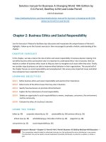
23. period 2 , symmetric about the origin
24. period 1, symmetric about the origin
s
3
2
s = tan t
1
2
1
1
2
t
0
1
2
3
26. period 4 , symmetric about the origin
25. period 4, symmetric about the s-axis
27. (a) Cos x and sec x are positive for x in the interval
2 , 2 ; and cos x and sec x are negative for x
in the intervals 32 , 2 and 2 , 32 . Sec x is
undefined when cos x is 0. The range of sec x is
(, 1] [1, ); the range of cos x is [1, 1].
Copyright 2014 Pearson Education, Inc.
Section 1.3 Trigonometric Functions
21
(b) Sin x and csc x are positive for x in the intervals
32 , and (0, ); and sin x and csc x are
negative for x in the intervals ( , 0) and
, 32 . Csc x is undefined when sin x is 0. The
range of csc x is (, 1] [1, ); the range of
sin x is [1, 1].
28. Since cot x tan1 x , cot x is undefined when tan x 0
and is zero when tan x is undefined. As tan x
approaches zero through positive values, cot x
approaches infinity. Also, cot x approaches negative
infinity as tan x approaches zero through negative
values.
29. D : x ; R : y 1, 0, 1
30. D : x ; R : y 1, 0, 1
31. cos x 2 cos x cos 2 sin x sin 2 (cos x)(0) (sin x)(1) sin x
32. cos x 2 cos x cos 2 sin x sin 2 (cos x)(0) (sin x)(1) sin x
33. sin x 2 sin x cos 2 cos x sin 2 (sin x)(0) (cos x)(1) cos x
34. sin x 2 sin x cos 2 cos x sin 2 (sin x)(0) (cos x)(1) cos x
35. cos( A B) cos( A ( B)) cos A cos( B) sin A sin( B) cos A cos B sin A( sin B)
cos A cos B sin A sin B
36. sin( A B ) sin( A ( B )) sin A cos( B ) cos A sin( B) sin A cos B cos A( sin B)
sin A cos B cos A sin B
37. If B A, A B 0 cos( A B) cos 0 1. Also cos( A B) cos( A A) cos A cos A sin A sin A
cos 2 A sin 2 A. Therefore, cos 2 A sin 2 A 1.
38. If B 2 , then cos( A 2 ) cos A cos 2 sin A sin 2 (cos A)(1) (sin A)(0) cos A and
sin( A 2 ) sin A cos 2 cos A sin 2 (sin A)(1) (cos A)(0) sin A . The result agrees with the fact that the
cosine and sine functions have period 2 .
39. cos( x) cos cos x sin sin x (1)(cos x) (0)(sin x) cos x
Copyright 2014 Pearson Education, Inc.
22
Chapter 1 Functions
40. sin(2 x) sin 2 cos( x) cos(2 ) sin( x ) (0)(cos( x)) (1)(sin( x)) sin x
41. sin 32 x sin 32 cos( x) cos 32 sin( x) ( 1)(cos x) (0)(sin( x)) cos x
42. cos 32 x cos 32 cos x sin 32 sin x (0)(cos x) (1)(sin x) sin x
43. sin 712 sin 4 3 sin 4 cos 3 cos 4 sin 3
2
2
cos 2 cos cos 2 sin sin 2
44. cos 11
12
4
3
4
3
4
3
6
4
3
2
2
2
1
2
2
2
2
3
2
2
2
1
2
2
4
6
12 22 23 22 12 23
cos cos cos sin sin
45. cos 12
3 4
3
4
3
4
46. sin 512 sin
47.
cos 2 8
23 4 sin 23 cos 4 cos 23 sin 4 23 22 12 22 12 23
1 cos
2
28 1
2
2
212 1
3
2
49. sin 2 12
1 cos
51. sin 2
3
4
2
2
2
sin
52. sin 2 cos 2
3
2
sin 2
cos 2
1 cos
1012 1 23 2
2 2
4
48.
2 3
4
1 cos
50. sin 2 38
2
cos 2 512
2
2
6
8
1 22 2
2
3
4
2
4
3 , 23 , 43 , 53
cos 2
cos 2
tan 2 1 tan 1 4 , 34 , 54 , 74
53. sin 2 cos 0 2sin cos cos 0 cos (2sin 1) 0 cos 0 or 2sin 1 0
cos 0 or sin 12 2 , 32 , or 6 , 56 6 , 2 , 56 , 32
54. cos 2 cos 0 2 cos 2 1 cos 0 2 cos 2 cos 1 0 (cos 1)(2 cos 1) 0
cos 1 0 or 2cos 1 0 cos 1 or cos 12 or 3 , 53 3 , , 53
55. tan( A B )
sin( A B )
cos( A B )
sin A cos B cos A cos B
cos A cos B sin A sin B
sin A cos B
cos A cos B
cos A cos B
cos A cos B
56. tan( A B)
sin( A B )
cos( A B )
sin A cos B cos A cos B
cos A cos B sin A sin B
sin A cos B
cos A cos B
cos A cos B
cos A cos B
cos A sin B
cos A cos B
sin A sin B
cos A cos B
1 tan A tan B
cos A sin B
cos A cos B
sin A sin B
cos A cos B
1 tan A tan B
tan A tan B
tan A tan B
57. According to the figure in the text, we have the following: By the law of cosines, c 2 a 2 b 2 2ab cos
12 12 2cos( A B ) 2 2cos( A B) . By distance formula, c 2 (cos A cos B)2 (sin A sin B)2
cos 2 A 2 cos A cos B cos 2 B sin 2 A 2sin A sin B sin 2 B 2 2(cos A cos B sin A sin B ) . Thus
c 2 2 2 cos( A B) 2 2(cos A cos B sin A sin B) cos( A B) cos A cos B sin A sin B .
Copyright 2014 Pearson Education, Inc.
Section 1.3 Trigonometric Functions
58. (a) cos( A B) cos A cos B sin A sin B
sin cos 2 and cos sin 2
Let A B
sin( A B) cos 2 ( A B) cos 2 A B cos 2 A cos B sin 2 A sin B
sin A cos B cos A sin B
(b) cos( A B ) cos A cos B sin A sin B
cos( A ( B)) cos A cos( B ) sin A sin( B )
cos( A B) cos A cos( B) sin A sin( B) cos A cos B sin A( sin B) cos A cos B sin A sin B
Because the cosine function is even and the sine functions is odd.
59. c 2 a 2 b 2 2ab cos C 22 32 2(2)(3) cos(60) 4 9 12 cos(60) 13 12
Thus, c 7 2.65.
12 7.
60. c 2 a 2 b 2 2ab cos C 22 32 2(2)(3) cos(40) 13 12 cos(40). Thus, c 13 12 cos 40° 1.951.
61. From the figures in the text, we see that sin B hc . If C is an acute angle, then sin C bh . On the other hand,
if C is obtuse (as in the figure on the right in the text), then sin C sin( C ) bh . Thus, in either case,
h b sin C c sin B ah ab sin C ac sin B.
By the law of cosines, cos C
a2 b2 c2
2ab
and cos B
a 2 c2 b2
.
2 ac
Moreover, since the sum of the interior
angles of triangle is , we have sin A sin( ( B C )) sin( B C ) sin B cos C cos B sin C
hc
a 2 b2 c2 a2 c 2 b2
2ac
2 ab
h (2a 2 b 2 c 2 c 2 b 2 ) ah ah bc sin A.
bh 2abc
bc
Combining our results we have ah ab sin C, ah ac sin B, and ah bc sin A. Dividing by abc gives
h sin A sin C sin B .
bc
a
c
b
law of sines
62. By the law of sines,
sin A
2
sin B
3
3/2
. By Exercise
c
59 we know that c 7. Thus sin B
3 3
2 7
0.982.
63. From the figure at the right and the law of cosines,
b 2 a 2 22 2(2a) cos B
a 2 4 4a
12 a2 2a 4.
Applying the law of sines to the figure,
2/2
a
3/2
b
b
3
2
sin A
a
sin B
b
a. Thus, combining results,
a 2 2a 4 b2 32 a 2 0 12 a 2 2a 4 0 a 2 4a 8 . From the quadratic formula and the fact that
a 0, we have a
4
42 4(1)( 8)
2
4 34
2
1.464.
64. (a) The graphs of y sin x and y x nearly coincide when x is near the origin (when the calculator is in
radians mode).
(b) In degree mode, when x is near zero degrees the sine of x is much closer to zero than x itself. The curves
look like intersecting straight lines near the origin when the calculator is in degree mode.
Copyright 2014 Pearson Education, Inc.
23
24
Chapter 1 Functions
65. A 2, B 2 , C , D 1
66. A 12 , B 2, C 1, D
1
2
67. A 2 , B 4, C 0, D 1
68.
A 2L , B L, C 0, D 0
69–72.
Example CAS commands:
Maple:
f : x - A*sin((2*Pi/B)*(x-C))D1;
A:3; C: 0; D1: 0;
f_list : [seq(f(x), B[1,3,2*Pi,5*Pi])];
plot(f_list, x -4*Pi..4*Pi, scaling constrained,
color [red,blue,green,cyan], linestyle [1,3,4,7],
legend ["B1", "B3","B2*Pi","B3*Pi"],
title "#69 (Section 1.3)");
Mathematica:
Clear[a, b, c, d, f, x]
f[x_]: a Sin[2/b (x c)] d
Plot[f[x]/.{a 3, b 1, c 0, d 0}, {x, 4, 4 }]
Copyright 2014 Pearson Education, Inc.
Section 1.3 Trigonometric Functions
69. (a) The graph stretches horizontally.
(b) The period remains the same: period | B |. The graph has a horizontal shift of 12 period.
70. (a) The graph is shifted right C units.
(b) The graph is shifted left C units.
(c) A shift of one period will produce no apparent shift. | C | 6
71. (a) The graph shifts upwards | D | units for D 0
(b) The graph shifts down | D | units for D 0.
72. (a) The graph stretches | A| units.
(b) For A 0, the graph is inverted.
Copyright 2014 Pearson Education, Inc.
25