Managerial economics and business strategy 8th edition solution manual baye prince
Bạn đang xem bản rút gọn của tài liệu. Xem và tải ngay bản đầy đủ của tài liệu tại đây (595.02 KB, 14 trang )
����������������������������������������������������������������������������������������������������������������������������������������������������������������������������������������������������������������������������������������������������������������������������������������������������������������������������������������������������������������������������������������������������������������������������������������������������������������������������������������������������������������������������������������������������������������������������������������������������������������������������������������������������������������������������������������������������������������������������������������������������������������������������������������������������������������������������������������������������������������������������������������������������������������������������������������������������������������������������������������������������������������������������������������������������������������������������������������������������������������������������������������������������������������������������������������������������������������������������������������������������������������������������������������������������������������������������������������������������������������������������������������������������������������������������������������������������������������������������������������������������������������������������������������������������������������������������������������������������������������������������������������������������������������������������������������������������������������������������������������������������������������������������������������������������������������������������������������������������������������������������������������������������������������������������������������������������������������������������������������������������������������������������������������������������������������������������������������������������������������������������������������������������������������������������������������������������������������������������������������������������������������������������������������������������������������������������������������������������������������������������������������������������������������������������������������������������������������������������������������������������������������������������������������������������������������������������������������������������������������������������������������������������������������������������������������������������������������������������������������������������������������������������������������������������������������������������������������������������������������������������������������������������������������������������������������������������������������������������������������������������������������������������������������������������������������������������������������������������������������������������������������������������������������������������������������������������������������������������������������������������������������������������������������������������������������������������������������������������������������������������������������������������������������������������������������������������������������������������������������������������������������������������������������������������������������������������������������������������������������������������������������������������������������������������������������������������������������������������������������������������������������������������������������������������������������������������������������������������������������������������������������������������������������������������������������������������������������������������������������������������������������������������������������������������������������������������������������������������������������������������������������������������������������������������������������������������������������������������������������������������������������will purchase 24 pounds of
store-label sugar and no producer-brand sugar. After the change, the consumer will
purchase no store-label sugar and 8 pounds of producer-brand sugar.
12.
See Figure 4-6. When there is no food stamp program, the market rate of substitution
is –0.33. The Food Stamp program leaves the market rate of substitution unchanged,
and a consumer can purchase $284 of food without spending her income. A dollarfor-dollar exchange of food stamps for money further expands a consumer’s
opportunity set, potentially making her better off.
Budget Constraint with and without Food Stamps
80
O 70
t
60
h
e 50
r
40
Budget line when food stamps are
sold on black market for $284
Budget line with $284 in food
stamps
G
30
o
o 20
d
s 10
Initial budget line
0
0
20
40
60
80
100
120
Food
Figure 4-6
4-5
140
160
180
200
220
240
Chapter 04 - The Theory of Individual Behavior
13.
See Figure 4-7. The offer expands the consumer’s budget set and allows her to
purchase more tires.
Budget Set with and without Buy 3, Get 4th Free Offer
Budget line with
“Buy 3, get the 4th
Free Offer”
400
350
300
250
Income
Spent on
200
Other
Goods
150
100
Initial budget line
50
0
0
2
4
6
Tires
Figure 4-7
4-6
8
10
12
14.
See Figure 4-8. The initial market rate of substitution is –0.5. Since, after the price
𝑃
decrease, the 𝑀𝑅𝑆 = −1 ≠ −0.67 = 𝑃𝐸𝑀 (where PEM is the price of electronic media
𝑇
and PT the price of travel) equilibrium has not been achieved. To reach equilibrium,
the business should increase its use of electronic media and decrease travel.
Budget Set
8
7
New budget line
6
5
Quantity 4
of
Travel 3
2
Initial budget line
1
0
0
-1
2
4
6
8
Quantity of Electronic Media
Figure 4-8
4-7
10
12
Chapter 04 - The Theory of Individual Behavior
15.
The impacts on the consumer’s budget sets are illustrated in Figure 4-9. As is shown
in the diagram, if the consumer has a strong preference for other goods (so that the
preferred quantity of other goods is greater than 10 units), the cash is preferred even
though it is taxed. Otherwise, the non-taxable, employer-sponsored health insurance
program allows an employee to achieve a higher indifference curve.
Budget Line with Employer Sponsored Health Insurance
14
Budget line with (taxable) cash
equivalent health insurance benefit
12
10
Other
Goods
Budget line with
health insurance
benefit
8
6
4
2
Initial budget line
0
0
1
2
3
4
5
6
7
8
9
Quantity of Health Insurance
Figure 4-9
16.
Under the existing plan, a worker that does not “goof off” produces 3 copiers per hour
and thus is paid $9 each hour. Under the new plan, each worker would be paid a flat
wage of $8 per hour. While it might appear on the surface that the company would
save $1 per hour in labor costs by switching plans, the flat wage would be a lousy
idea. Under the current plan, workers get paid the $9 only if they work hard during
the hour and produce 3 machines that pass inspection. Under the new plan, workers
would get paid $8 an hour regardless of how many units they produce. Since your
firm has no supervisors to monitor the workers, you should not favor the plan.
4-8
17.
As shown in Figure 4-10, the budget line when more than 10 dozen bagels are
purchased annually under the frequent buyer program is always greater than the
budget line when the firm sells each dozen bagels at a 3 percent discount. However,
the budget line for consumers who purchase fewer than 10 dozen bagels per year is
greater under the 3 percent per dozen discount.
Comparison of Budget Lines Under Different Offers
250
Budget line under the
frequent buyer
program
200
Income 150
Spent on
Other
Goods 100
Budget line with
3 percent
discount
50
0
0
5
10
15
20
25
30
35
Quantity of Bagels (dozens)
Figure 4-10
18.
Yes. Since pizza is an inferior good, if the consumer is given $50 in cash she will
definitely spend it entirely on music downloads – just as she would if given a $50 gift
certificate for music downloads.
4-9
Chapter 04 - The Theory of Individual Behavior
19.
Figure 4-11 illustrates a consumer’s budget line when a firm offers a “quantity
discount.” A consumer will never purchase exactly 8 bottles of wine, since at this
kink in the opportunity set the consumer would always be better off by buying more
or less wine.
Budget Line with Quantity Discount
250
200
Quantity
of Other
Goods
150
100
50
0
0
5
10
Quantity of Wine
Figure 4-11
4-10
15
20
20.
Figure 4-12 contains profit as a function of output. Output when managers are
compensated based solely on output is 20 units and profits are zero. In contrast, when
managers’ compensation is based solely on profits, output is 10 units and profits are
$200. When managers’ compensation is based on a combination of output and profit,
output ranges between 10 and 20 units and profit will be between zero and $200. The
exact combination of output and profit depends on how these variables are weighted.
250
200
150
Profits ($)
100
50
0
0
5
10
15
20
25
Output
Figure 4-12
21.
Figures 4-13a and 4-13b, respectively, illustrate Albert’s and Sid’s opportunity sets.
Since there are 24 hours per day, at the new wage rate of $22 per hour Albert will
supply 14 hours of labor per day (24-10), and Sid will supply 10 hours of labor per
day (24-14). This seemingly contradictory result is explained by decomposing the
wage change into the substitution effect and income effect. The diminishing marginal
rate of substitution between income and leisure implies that the substitution effect
will increase the amount of leisure consumed by each worker (decrease the amount of
labor supplied). Since after the wage change Albert is observed consuming less
leisure (supplying more labor), the income effect dominates the substitution effect. In
contrast, the substitution effect dominates the income effect for Sid; since Sid is
observed consuming more leisure (supplying less labor) after the wage change.
4-11
Chapter 04 - The Theory of Individual Behavior
Albert’s Opportunity Set
700
600
500
400
Income
300
200
100
0
0
5
10
15
20
25
30
Leisure Hours
Figure 4-13a
Sid’s Opportunity Set
700
600
500
400
Income
300
200
100
0
0
5
10
15
Leisure Hours
Figure 4-13b
4-12
20
25
30
22.
Gift cards are not merely a fad. Retailers experience significant benefits from gift
cards since they minimize product returns; independent of whether the good is normal
or inferior. Gift cards can also benefit consumers. A gift card does not impact the
amount purchased for one good (say the good on the Y axis), but shifts out the budget
constraint for the other good (the good on the X axis) by the face value of the gift
card. The expanded budget constraint permits the consumer to reach a higher
indifference curve; resulting in greater utility.
23.
AOG
Flat-Rate Plan
Old Plan
3,500
AOG
A
10,000
3,500
10,000
Under the Old Plan, consumers consumed 3,500 gigabytes of Internet traffic for
£399.99. The budget line under the Flat-Rate Plan, however, is significantly different.
Consumers can choose to now spend all their income on all other goods (AOG),
represented by point A on the AOG axis, or consume the same amount of AOG as
they did under the old plan along with any amount of Internet traffic up to the
maximum volume in a month. Optimizing consumers will choose the corner solution
represented by the same number of units of AOG as the Old Plan and 10,000
gigabytes of broadband Internet traffic. Thus, UK consumers are necessarily better
off (assuming similar quality of service). The Internet service provider (ISP),
however, gains no additional revenues and presumably must increase it network
capacity. Therefore, the ISP may earn lower profit (ignoring other factors).
4-13
Chapter 04 - The Theory of Individual Behavior
24.
The movement from selling 9 bottles of Coke to 7 bottles of Coke, as shown in the
graph, is the change in sales due to the substitution effect. We know this because it is
determined by keeping the consumer on the same indifference curve, and comparing
purchases at the two different prices. The price increase also has an income effect,
since it effectively lowers the consumer’s overall purchasing power. Since Coke is a
normal good, this lowering of income results in lower sales. Adding this to the
substitution effect means that sales will be less than 7.
25.
As shown in the book, we can determine aggregate demand by summing up quantity
demanded for each individual at every price. At a given price, P, quantity demanded
by a female customer is 24 – 2*P, and at that same price, quantity demanded by a
male customer is 27 – P. Summing gives us 24 – 2*P + 27 – P = 51 – 3P. So, for any
price P, the total demand is 51 – 3P. If we call total demand QT, then we have the
aggregate demand equation: QT = 51 – 3P. We often want to graph demand using the
inverse demand function, and we can do that here. Solving the aggregate demand
curve for P gives us: P = 17 – (1/3)*QT.
More download links:
managerial economics and business strategy 8th edition solution manual
managerial economics and business strategy test bank pdf
managerial economics and business strategy 8th edition chapter 3 answers
managerial economics and business strategy chapter 1 answers
managerial economics and business strategy 8th edition chapter 5 answers
managerial economics and business strategy 7th edition solutions
managerial economics and business strategy 8th edition chapter 8 answers
managerial economics and business strategy 8e chapter 1 answers
managerial economics and business strategy 8th edition chapter 2 answers
4-14