Solution manual for differential equations and linear algebra 3rd edition by edwards
Bạn đang xem bản rút gọn của tài liệu. Xem và tải ngay bản đầy đủ của tài liệu tại đây (1.02 MB, 68 trang )
CHAPTER 1
FIRST-ORDER DIFFERENTIAL EQUATIONS
SECTION 1.1
DIFFERENTIAL EQUATIONS AND MATHEMATICAL MODELS
The main purpose of Section 1.1 is simply to introduce the basic notation and terminology of
differential equations, and to show the student what is meant by a solution of a differential
equation. Also, the use of differential equations in the mathematical modeling of real-world
phenomena is outlined.
Problems 1–12 are routine verifications by direct substitution of the suggested solutions into the
given differential equations. We include here just some typical examples of such verifications.
3.
If y1 = cos 2 x and y2 = sin 2 x , then y1′ = − 2sin 2 x and y2′ = 2 cos 2 x so
y1′′ = − 4cos 2 x = − 4 y1
and
y2′′ = − 4sin 2 x = − 4 y2 .
Thus y1′′ + 4 y1 = 0 and y2′′ + 4 y2 = 0.
4.
If y1 = e3 x and y2 = e −3 x , then y1 = 3 e3 x and y2 = − 3 e −3 x so
y1′′ = 9 e3 x = 9 y1
5.
and
y2′′ = 9 e −3 x = 9 y2 .
If y = e x − e − x , then y′ = e x + e − x so y′ − y = ( e x + e − x ) − ( e x − e − x ) = 2 e − x . Thus
y′ = y + 2 e − x .
6.
If y1 = e −2 x and y2 = x e −2 x , then y1′ = − 2 e −2 x , y1′′ = 4 e −2 x , y2′ = e −2 x − 2 x e −2 x , and
y2′′ = − 4 e −2 x + 4 x e −2 x . Hence
y1′′ + 4 y1′ + 4 y1 = ( 4 e −2 x ) + 4 ( −2 e −2 x ) + 4 ( e −2 x ) = 0
and
y2′′ + 4 y2′ + 4 y2 =
( − 4e
−2 x
+ 4 x e −2 x ) + 4 ( e −2 x − 2 x e −2 x ) + 4 ( x e −2 x ) = 0.
Section 1.1
Copyright © 2010 Pearson Education, Inc. Publishing as Prentice Hall.
1
8.
If y1 = cos x − cos 2 x and y2 = sin x − cos 2 x, then y1′ = − sin x + 2sin 2 x,
y1′′ = − cos x + 4 cos 2 x, and y2′ = cos x + 2sin 2 x, y2′′ = − sin x + 4 cos 2 x. Hence
y1′′ + y1 = ( − cos x + 4 cos 2 x ) + ( cos x − cos 2 x ) = 3cos 2 x
and
y2′′ + y2 = ( − sin x + 4 cos 2 x ) + ( sin x − cos 2 x ) = 3cos 2 x.
11.
If y = y1 = x −2 then y′ = − 2 x −3 and y ′′ = 6 x −4 , so
x 2 y ′′ + 5 x y ′ + 4 y = x 2 ( 6 x −4 ) + 5 x ( −2 x −3 ) + 4 ( x −2 ) = 0.
If y = y2 = x −2 ln x then y′ = x −3 − 2 x −3 ln x and y ′′ = − 5 x −4 + 6 x −4 ln x, so
x 2 y ′′ + 5 x y ′ + 4 y = x 2 ( −5 x −4 + 6 x −4 ln x ) + 5 x ( x −3 − 2 x −3 ln x ) + 4 ( x −2 ln x )
= ( −5 x −2 + 5 x −2 ) + ( 6 x −2 − 10 x −2 + 4 x −2 ) ln x = 0.
13.
Substitution of y = e rx into 3 y ′ = 2 y gives the equation 3r e rx = 2 e rx that simplifies
to 3 r = 2. Thus r = 2/3.
14.
Substitution of y = e rx into 4 y ′′ = y gives the equation 4r 2 e rx = e rx that simplifies to
4 r 2 = 1. Thus r = ± 1/ 2.
15.
Substitution of y = e rx into y′′ + y ′ − 2 y = 0 gives the equation r 2e rx + r e rx − 2 e rx = 0
that simplifies to r 2 + r − 2 = ( r + 2)( r − 1) = 0. Thus r = –2 or r = 1.
16.
Substitution of y = e rx into 3 y ′′ + 3 y ′ − 4 y = 0 gives the equation
3r 2 e rx + 3r e rx − 4 e rx = 0 that simplifies to 3r 2 + 3r − 4 = 0. The quadratic formula then
(
)
gives the solutions r = −3 ± 57 / 6.
The verifications of the suggested solutions in Problems 17–26 are similar to those in Problems
1–12. We illustrate the determination of the value of C only in some typical cases. However,
we illustrate typical solution curves for each of these problems.
2
Chapter 1
Copyright © 2010 Pearson Education, Inc. Publishing as Prentice Hall.
C = 2
17.
C = 3
18.
5
5
(0,3)
0
−5
−5
y
y
(0,2)
0
x
0
−5
−5
5
0
x
5
If y ( x ) = C e x − 1 then y(0) = 5 gives C – 1 = 5, so C = 6. The figure is on the
left below.
19.
20
10
(0,5)
(0,10)
y
y
5
0
0
−5
−10
−5
0
x
5
−20
−10
−5
0
x
5
10
20.
If y ( x ) = C e − x + x − 1 then y(0) = 10 gives C – 1 = 10, so C = 11. The figure is
on the right above.
21.
C = 7. The figure is on the left at the top of the next page.
Section 1.1
Copyright © 2010 Pearson Education, Inc. Publishing as Prentice Hall.
3
5
10
(0,7)
0
0
y
y
5
(0,0)
−5
−10
−2
−1
0
x
1
2
−5
−20
−10
0
x
10
20
22.
If y ( x ) = ln( x + C ) then y(0) = 0 gives ln C = 0, so C = 1. The figure is on the
right above.
23.
If y ( x ) = 14 x 5 + C x −2 then y(2) = 1 gives the equation
solution C = –56. The figure is on the left below.
30
30
20
20
10
10
y
y
−10
−20
0
1
2
3
x
4
0
−10
−20
24.
⋅ 32 + C ⋅ 18 = 1 with
(1,1)
(2,1)
0
−30
1
4
−30
0
0.5
1
1.5
2
2.5
x
C = 17. The figure is on the right above.
Chapter 1
Copyright © 2010 Pearson Education, Inc. Publishing as Prentice Hall.
3
3.5
4
4.5
5
25.
If y ( x ) = tan( x 2 + C ) then y(0) = 1 gives the equation tan C = 1. Hence one value
of C is C = π / 4 (as is this value plus any integral multiple of π).
4
2
y
(0,1)
0
−2
−4
−2
26.
−1
0
x
1
2
Substitution of x = π and y = 0 into y = ( x + C ) cos x yields the equation
0 = (π + C )( −1), so C = − π .
10
5
y
(π,0)
0
−5
−10
27.
0
5
x
10
y′ = x + y
Section 1.1
Copyright © 2010 Pearson Education, Inc. Publishing as Prentice Hall.
5
28.
The slope of the line through ( x, y ) and ( x / 2, 0) is y′ = ( y − 0) /( x − x / 2) = 2 y / x,
so the differential equation is x y ′ = 2 y.
29.
If m = y′ is the slope of the tangent line and m′ is the slope of the normal line at
( x, y ), then the relation m m′ = − 1 yields m′ = 1/ y ′ = ( y − 1) /( x − 0). Solution for
y′ then gives the differential equation (1 − y ) y ′ = x.
30.
Here m = y ′ and m′ = Dx ( x 2 + k ) = 2 x, so the orthogonality relation m m′ = − 1 gives
the differential equation 2 x y′ = − 1.
31.
The slope of the line through ( x, y ) and ( − y , x ) is y′ = ( x − y ) /( − y − x ), so the
differential equation is ( x + y ) y ′ = y − x.
In Problems 32–36 we get the desired differential equation when we replace the "time rate of
change" of the dependent variable with its derivative, the word "is" with the = sign, the phrase
"proportional to" with k, and finally translate the remainder of the given sentence into symbols.
32.
dP / dt = k P
33.
dv / dt = k v 2
34.
dv / dt = k (250 − v )
35.
dN / dt = k ( P − N )
36.
dN / dt = k N ( P − N )
37.
The second derivative of any linear function is zero, so we spot the two solutions
y ( x ) ≡ 1 or y ( x ) = x of the differential equation y′′ = 0.
38.
A function whose derivative equals itself, and hence a solution of the differential
equation y′ = y is y ( x ) = e x .
39.
We reason that if y = kx 2 , then each term in the differential equation is a multiple of x 2 .
The choice k = 1 balances the equation, and provides the solution y ( x ) = x 2 .
40.
If y is a constant, then y′ ≡ 0 so the differential equation reduces to y 2 = 1. This gives
the two constant-valued solutions y ( x ) ≡ 1 and y ( x ) ≡ − 1.
6
Chapter 1
Copyright © 2010 Pearson Education, Inc. Publishing as Prentice Hall.
41.
We reason that if y = ke x , then each term in the differential equation is a multiple of e x .
The choice k = 12 balances the equation, and provides the solution y ( x ) = 12 e x .
42.
Two functions, each equaling the negative of its own second derivative, are the two
solutions y ( x ) = cos x and y ( x ) = sin x of the differential equation y ′′ = − y.
43.
(a)
We need only substitute x (t ) = 1/(C − kt ) in both sides of the differential
equation x′ = kx 2 for a routine verification.
(b)
The zero-valued function x (t ) ≡ 0 obviously satisfies the initial value problem
x′ = kx 2 , x (0) = 0.
(a)
The figure on the left below shows typical graphs of solutions of the differential
equation x′ = 12 x 2 .
44.
5
6
5
4
4
x
x
3
3
2
2
1
1
0
0
0
1
2
t
3
4
0
1
2
t
3
4
(b)
The figure on the right above shows typical graphs of solutions of the differential
equation x′ = − 12 x 2 . We see that — whereas the graphs with k = 12 appear to "diverge
to infinity" — each solution with k = − 12 appears to approach 0 as t → ∞. Indeed, we
see from the Problem 43(a) solution x (t ) = 1/(C − 12 t ) that x (t ) → ∞ as t → 2C.
However, with k = − 12 it is clear from the resulting solution x (t ) = 1/(C + 12 t ) that
x (t ) remains bounded on any finite interval, but x (t ) → 0 as t → +∞.
45.
1
,
Substitution of P′ = 1 and P = 10 into the differential equation P′ = kP 2 gives k = 100
so Problem 43(a) yields a solution of the form P (t ) = 1/(C − t /100). The initial
condition P (0) = 2 now yields C = 12 , so we get the solution
Section 1.1
Copyright © 2010 Pearson Education, Inc. Publishing as Prentice Hall.
7
P(t ) =
1
t
1
−
2 100
=
100
.
50 − t
We now find readily that P = 100 when t = 49, and that P = 1000 when t = 49.9.
It appears that P grows without bound (and thus "explodes") as t approaches 50.
46.
Substitution of v′ = −1 and v = 5 into the differential equation v′ = kv 2 gives
k = − 251 , so Problem 43(a) yields a solution of the form v (t ) = 1/(C + t / 25). The initial
condition v (0) = 10 now yields C = 101 , so we get the solution
v (t ) =
1
t
1
+
10 25
=
50
.
5 + 2t
We now find readily that v = 1 when t = 22.5, and that v = 0.1 when t = 247.5.
It appears that v approaches 0 as t increases without bound. Thus the boat gradually
slows, but never comes to a "full stop" in a finite period of time.
47.
(a)
y (10) = 10 yields 10 = 1/(C − 10), so C = 101/10.
(b)
There is no such value of C, but the constant function y ( x ) ≡ 0 satisfies the
conditions y′ = y 2 and y (0) = 0.
(c)
It is obvious visually (in Fig. 1.1.8 of the text) that one and only one solution
curve passes through each point ( a , b) of the xy-plane, so it follows that there exists a
unique solution to the initial value problem y ′ = y 2 , y (a ) = b.
48.
(b)
Obviously the functions u( x ) = − x 4 and v ( x ) = + x 4 both satisfy the differential
equation xy ′ = 4 y. But their derivatives u′( x ) = − 4 x 3 and v′( x ) = + 4 x 3 match at
x = 0, where both are zero. Hence the given piecewise-defined function y ( x ) is
differentiable, and therefore satisfies the differential equation because u ( x ) and v ( x )
do so (for x ≤ 0 and x ≥ 0, respectively).
(c)
If a ≥ 0 (for instance), choose C+ fixed so that C+ a 4 = b. Then the function
C x 4
y( x) = − 4
C+ x
if x ≤ 0,
if x ≥ 0
satisfies the given differential equation for every real number value of C− .
8
Chapter 1
Copyright © 2010 Pearson Education, Inc. Publishing as Prentice Hall.
SECTION 1.2
INTEGRALS AS GENERAL AND PARTICULAR SOLUTIONS
This section introduces general solutions and particular solutions in the very simplest situation
— a differential equation of the form y ′= f ( x ) — where only direct integration and evaluation
of the constant of integration are involved. Students should review carefully the elementary
concepts of velocity and acceleration, as well as the fps and mks unit systems.
1.
Integration of y′ = 2 x + 1 yields y ( x ) =
∫ (2 x + 1) dx
= x 2 + x + C. Then substitution
of x = 0, y = 3 gives 3 = 0 + 0 + C = C, so y ( x ) = x 2 + x + 3.
2.
∫ ( x − 2)
Integration of y ′ = ( x − 2)2 yields y ( x ) =
2
dx =
1
3
( x − 2)3 + C. Then
substitution of x = 2, y = 1 gives 1 = 0 + C = C, so y ( x ) =
3.
Integration of y ′ = x yields y ( x ) =
∫
x dx =
x = 4, y = 0 gives 0 = 163 + C , so y ( x ) =
4.
Integration of y′ = x −2 yields y ( x ) =
∫x
2
3
−2
2
3
1
3
( x − 2)3 + 1.
x 3/ 2 + C. Then substitution of
( x 3/ 2 − 8).
dx = − 1/ x + C. Then substitution of
x = 1, y = 5 gives 5 = − 1 + C , so y ( x ) = − 1/ x + 6.
5.
∫ ( x + 2)
Integration of y′ = ( x + 2) −1/ 2 yields y ( x ) =
−1/ 2
dx = 2 x + 2 + C. Then
substitution of x = 2, y = − 1 gives −1 = 2 ⋅ 2 + C , so y ( x ) = 2 x + 2 − 5.
6.
Integration of y′ = x ( x 2 + 9)1/ 2 yields y ( x ) =
∫ x (x
2
+ 9)1/ 2 dx =
1
3
( x 2 + 9)3/ 2 + C.
Then substitution of x = − 4, y = 0 gives 0 = 13 (5)3 + C , so
y( x) =
7.
1
3
( x 2 + 9)3/ 2 − 125 .
∫ 10 /( x
Integration of y ′ = 10 /( x 2 + 1) yields y ( x ) =
2
+ 1) dx = 10 tan −1 x + C. Then
substitution of x = 0, y = 0 gives 0 = 10 ⋅ 0 + C , so y ( x ) = 10 tan −1 x.
8.
9.
Integration of y′ = cos 2 x yields y ( x ) =
∫ cos 2 x dx
of x = 0, y = 1 gives 1 = 0 + C , so y ( x ) =
1
2
Integration of y′ = 1/ 1 − x 2 yields y ( x ) =
∫ 1/
=
1
2
sin 2 x + C. Then substitution
sin 2 x + 1.
1 − x 2 dx = sin −1 x + C. Then
substitution of x = 0, y = 0 gives 0 = 0 + C , so y ( x ) = sin −1 x.
Section 1.2
Copyright © 2010 Pearson Education, Inc. Publishing as Prentice Hall.
9
10.
Integration of y′ = x e − x yields
y( x) =
∫ xe
−x
∫ue
dx =
u
du = (u − 1)eu = − ( x + 1) e − x + C
(when we substitute u = − x and apply Formula #46 inside the back cover of the
textbook). Then substitution of x = 0, y = 1 gives 1 = − 1 + C , so
y ( x ) = − ( x + 1) e − x + 2.
11.
If a (t ) = 50 then v (t ) =
x (t ) =
12.
∫ ( −20) dt
3 2
2
t + 5) dt =
∫ (t
2
= − 20 t + v0 = − 20 t − 15. Hence
− 10 t 2 − 15 t + x0 = − 10 t 2 − 15 t + 5.
∫ 3t dt
If a (t ) = 2 t + 1 then v (t ) =
x (t ) =
15.
∫(
= 50 t + v0 = 50 t + 10. Hence
25 t 2 + 10 t + x0 = 25 t 2 + 10 t + 20.
∫ ( −20 t − 15) dt =
If a (t ) = 3 t then v (t ) =
x (t ) =
14.
∫ (50 t + 10) dt =
If a (t ) = − 20 then v (t ) =
x (t ) =
13.
∫ 50 dt
3 2
2
=
3 2
2
t + v0 =
1 3
2
t + 5 t + x0 =
∫ (2 t + 1) dt
t + 5. Hence
1 3
2
t + 5 t.
= t 2 + t + v0 = t 2 + t − 7. Hence
1 3
3
+ t − 7) dt =
t + 21 t − 7t + x0 =
If a (t ) = 4(t + 3) 2 . then v (t ) =
∫ 4(t + 3)
2
dt =
4
3
1 3
3
t + 12 t − 7t + 4.
(t + 3)3 + C =
4
3
(t + 3)3 − 37 (taking
C = –37 so that v(0) = –1). Hence
x (t ) =
16.
∫
4
3
(t + 3)3 − 37 dt =
If a (t ) = 1/ t + 4 then v (t ) =
1
3
∫ 1/
(t + 3) 4 − 37t + C =
1
3
(t + 3) 4 − 37t − 26.
t + 4 dt = 2 t + 4 + C = 2 t + 4 − 5 (taking
C = –5 so that v(0) = –1). Hence
x (t ) =
∫ (2
t + 4 − 5) dt =
4
3
(t + 4)3/ 2 − 5 t + C =
4
3
(t + 4)3/ 2 − 5 t − 293
(taking C = − 29 / 3 so that x (0) = 1 ).
10
Chapter 1
Copyright © 2010 Pearson Education, Inc. Publishing as Prentice Hall.
17.
If a (t ) = (t + 1) −3 then v (t ) =
(taking C =
1
2
x (t ) =
∫ (t + 1)
−3
dt = − 12 (t + 1) −2 + C = − 12 (t + 1) −2 + 12
so that v(0) = 0). Hence
∫ −
1
2
(t + 1) −2 + 12 dt =
1
2
(t + 1) −1 + 12 t + C =
1
2
(t + 1) −1 + t − 1
(taking C = − 12 so that x (0) = 0 ).
18.
If a (t ) = 50sin 5t then v (t ) =
∫ 50sin 5t dt
= − 10cos5t + C = − 10cos 5t (taking
C = 0 so that v(0) = –10). Hence
x (t ) =
∫ ( −10cos 5t ) dt =
− 2sin 5t + C = − 2sin 5t + 10
(taking C = − 10 so that x (0) = 8 ).
Note that v (t ) = 5 for 0 ≤ t ≤ 5 and that v (t ) = 10 − t for 5 ≤ t ≤ 10. Hence
x (t ) = 5t + C1 for 0 ≤ t ≤ 5 and x (t ) = 10t − 12 t 2 + C2 for 5 ≤ t ≤ 10. Now C1 = 0
because x (0) = 0, and continuity of x (t ) requires that x (t ) = 5t and
x (t ) = 10t − 12 t 2 + C2 agree when t = 5. This implies that C2 = − 252 , and we get the
following graph.
40
30
(5,25)
v
19.
20
10
0
0
2
4
6
8
10
t
Section 1.2
Copyright © 2010 Pearson Education, Inc. Publishing as Prentice Hall.
11
Note that v (t ) = t for 0 ≤ t ≤ 5 and that v (t ) = 5 for 5 ≤ t ≤ 10. Hence x (t ) = 12 t 2 + C1
for 0 ≤ t ≤ 5 and x (t ) = 5t + C2 for 5 ≤ t ≤ 10. Now C1 = 0 because x (0) = 0, and
20.
continuity of x (t ) requires that x (t ) = 12 t 2 and x (t ) = 5t + C2 agree when t = 5.
40
40
30
30
20
20
v
v
This implies that C2 = − 252 , and we get the graph on the left below.
(5,12.5)
(5,12.5)
10
0
0
2
4
6
10
8
10
t
21.
0
0
2
4
6
8
10
t
Note that v (t ) = t for 0 ≤ t ≤ 5 and that v (t ) = 10 − t for 5 ≤ t ≤ 10. Hence
x (t ) = 12 t 2 + C1 for 0 ≤ t ≤ 5 and x (t ) = 10t − 12 t 2 + C2 for 5 ≤ t ≤ 10. Now C1 = 0
because x (0) = 0, and continuity of x (t ) requires that x (t ) = 12 t 2 and
x (t ) = 10t − 12 t 2 + C2 agree when t = 5. This implies that C2 = −25, and we get the
graph on the right above.
22.
For 0 ≤ t ≤ 3 : v (t ) = 53 t so x (t ) = 56 t 2 + C1. Now C1 = 0 because x (0) = 0, so
x (t ) = 65 t 2 on this first interval, and its right endpoint value is x (3) = 7 12 .
For 3 ≤ t ≤ 7 : v (t ) = 5 so x (t ) = 5t + C2 . Now x (3) = 7 12 implies that C2 = −7 12 ,
so x (t ) = 5t − 7 12 on this second interval, where its right endpoint value is x (7) = 27 12 .
For 7 ≤ t ≤ 10 : v − 5 = − 53 (t − 7), so v (t ) = − 53 t + 503 . Hence x (t ) = − 65 t 2 + 503 t + C3 ,
2
1
and x (7) = 27 12 implies that C3 = − 290
6 . Finally, x ( t ) = 6 ( −5t + 100t − 290) on this
third interval, and we get the graph at the top of the next page.
12
Chapter 1
Copyright © 2010 Pearson Education, Inc. Publishing as Prentice Hall.
40
30
v
(7,27.5)
20
10
(3,7.5)
0
0
2
4
6
8
10
t
23.
v = –9.8t + 49, so the ball reaches its maximum height (v = 0) after t = 5 seconds. Its
maximum height then is y(5) = –4.9(5)2 + 49(5) = 122.5 meters.
24.
v = –32t and y = –16t2 + 400, so the ball hits the ground (y = 0) when
t = 5 sec, and then v = –32(5) = –160 ft/sec.
25.
a = –10 m/s2 and v0 = 100 km/h ≈ 27.78 m/s, so v = –10t + 27.78, and hence
x(t) = –5t2 + 27.78t. The car stops when v = 0, t ≈ 2.78, and thus the distance
traveled before stopping is x(2.78) ≈ 38.59 meters.
26.
v = –9.8t + 100 and y = –4.9t2 + 100t + 20.
(a)
v = 0 when t = 100/9.8 so the projectile's maximum height is
y(100/9.8) = –4.9(100/9.8)2 + 100(100/9.8) + 20 ≈ 530 meters.
(b)
It passes the top of the building when y(t) = –4.9t2 + 100t + 20 = 20,
and hence after t = 100/4.9 ≈ 20.41 seconds.
(c)
The roots of the quadratic equation y(t) = –4.9t2 + 100t + 20 = 0 are
t = –0.20, 20.61. Hence the projectile is in the air 20.61 seconds.
27.
a = –9.8 m/s2 so v = –9.8 t – 10 and
y = –4.9 t2 – 10 t + y0.
The ball hits the ground when y = 0 and
v = –9.8 t – 10 = –60,
so t ≈ 5.10 s. Hence
y0 = 4.9(5.10)2 + 10(5.10) ≈ 178.57 m.
Section 1.2
Copyright © 2010 Pearson Education, Inc. Publishing as Prentice Hall.
13
28.
v = –32t – 40 and y = –16t2 – 40t + 555. The ball hits the ground (y = 0) when t ≈
4.77 sec, with velocity v = v(4.77) ≈ –192.64 ft/sec, an impact speed of about 131
mph.
29.
Integration of dv/dt = 0.12 t3 + 0.6 t, v(0) = 0 gives v(t) = 0.3 t2 + 0.04 t3. Hence
v(10) = 70. Then integration of dx/dt = 0.3 t2 + 0.04 t3, x(0) = 0 gives
x(t) = 0.1 t3 + 0.04 t4, so x(10) = 200. Thus after 10 seconds the car has gone 200 ft and
is traveling at 70 ft/sec.
30.
Taking x0 = 0 and v0 = 60 mph = 88 ft/sec, we get
v = –at + 88,
and v = 0 yields t = 88/a. Substituting this value of t and x = 176 in
x = –at2/2 + 88t,
we solve for a = 22 ft/sec2. Hence the car skids for t = 88/22 = 4 sec.
31.
If a = –20 m/sec2 and x0 = 0 then the car's velocity and position at time t are given
by
v = –20t + v0, x = –10 t2 + v0t.
It stops when v = 0 (so v0 = 20t), and hence when
x = 75 = –10 t2 + (20t)t = 10 t2.
Thus t =
7.5 sec so
v0 = 20 7.5 ≈ 54.77 m/sec ≈ 197 km/hr.
32.
Starting with x0 = 0 and v0 = 50 km/h = 5×10⁴ m/h, we find by the method of
Problem 30 that the car's deceleration is a = (25/3)×107 m/h2. Then, starting with x0 =
0 and v0 = 100 km/h = 105 m/h, we substitute t = v0/a into
x = – 12 at2 + v0t
and find that x = 60 m when v = 0. Thus doubling the initial velocity quadruples the
distance the car skids.
33.
If v0 = 0 and y0 = 20 then
v = –at and y = – 12 at2 + 20.
Substitution of t = 2, y = 0 yields a = 10 ft/sec2. If v0 = 0 and
14
Chapter 1
Copyright © 2010 Pearson Education, Inc. Publishing as Prentice Hall.
y0 = 200 then
v = –10t and y = –5t2 + 200.
Hence y = 0 when t =
34.
40 = 2 10 sec and v = –20 10 ≈ –63.25 ft/sec.
On Earth: v = –32t + v0, so t = v0/32 at maximum height (when v = 0).
Substituting this value of t and y = 144 in
y = –16t2 + v0t,
we solve for v0 = 96 ft/sec as the initial speed with which the person can throw a ball
straight upward.
On Planet Gzyx: From Problem 27, the surface gravitational acceleration on planet
Gzyx is a = 10 ft/sec2, so
v = –10t + 96
and
y = –5t2 + 96t.
Therefore v = 0 yields t = 9.6 sec, and thence ymax = y(9.6) = 460.8 ft is the
height a ball will reach if its initial velocity is 96 ft/sec.
35.
If v0 = 0 and y0 = h then the stone′s velocity and height are given by
v = –gt,
Hence y = 0 when t =
y = –0.5 gt2 + h.
2h / g so
v = –g 2h / g = – 2gh .
36.
The method of solution is precisely the same as that in Problem 30. We find first that, on
Earth, the woman must jump straight upward with initial velocity v0 = 12 ft/sec to
reach a maximum height of 2.25 ft. Then we find that, on the Moon, this initial velocity
yields a maximum height of about 13.58 ft.
37.
We use units of miles and hours. If x0 = v0 = 0 then the car′s velocity and position
after t hours are given by
v = at, x = 12 t2.
Since v = 60 when t = 5/6, the velocity equation yields a = 72 mi/hr2. Hence the
distance traveled by 12:50 pm is
x = (0.5)(72)(5/6)2 = 25 miles.
Section 1.2
Copyright © 2010 Pearson Education, Inc. Publishing as Prentice Hall.
15
38.
Again we have
v = at,
x =
1 2
2
t.
But now v = 60 when x = 35. Substitution of a = 60/t (from the velocity equation)
into the position equation yields
35 = (0.5)(60/t)(t2) = 30t,
whence t = 7/6 hr, that is, 1:10 p.m.
39.
Integration of y′ = (9/vS)(1 – 4x2) yields
y = (3/vS)(3x – 4x3) + C,
and the initial condition y(–1/2) = 0 gives C = 3/vS. Hence the swimmer′s trajectory
is
y(x) = (3/vS)(3x – 4x3 + 1).
Substitution of y(1/2) = 1 now gives vS = 6 mph.
40.
Integration of y′ = 3(1 – 16x4) yields
y = 3x – (48/5)x5 + C,
and the initial condition y(–1/2) = 0 gives C = 6/5. Hence the swimmer′s trajectory
is
y(x) = (1/5)(15x – 48x5 + 6),
so his downstream drift is y(1/2) = 2.4 miles.
41.
The bomb equations are a = −32, v = −32, and sB = s = −16t 2 + 800, with t = 0 at the
instant the bomb is dropped. The projectile is fired at time t = 2, so its corresponding
equations are a = −32, v = −32(t − 2) + v0 , and
sP = s = − 16(t − 2)2 + v0 (t − 2)
for t ≥ 2 (the arbitrary constant vanishing because sP (2) = 0 ). Now the condition
sB (t ) = −16t 2 + 800 = 400 gives t = 5, and then the requirement that sP (5) = 400 also
yields v0 = 544 / 3 ≈ 181.33 ft/s for the projectile's needed initial velocity.
42.
16
Let x (t ) be the (positive) altitude (in miles) of the spacecraft at time t (hours), with
t = 0 corresponding to the time at which its retrorockets are fired; let v (t ) = x′(t ) be
Chapter 1
Copyright © 2010 Pearson Education, Inc. Publishing as Prentice Hall.
the velocity of the spacecraft at time t. Then v0 = −1000 and x0 = x (0) is unknown.
But the (constant) acceleration is a = +20000, so
v (t ) = 20000 t − 1000
and
x (t ) = 10000 t 2 − 1000 t + x0 .
Now v (t ) = 20000t − 1000 = 0 (soft touchdown) when t =
3 minutes of descent). Finally, the condition
1
20
hr (that is, after exactly
0 = x ( 201 ) = 10000( 201 ) 2 − 1000( 201 ) + x0
yields x0 = 25 miles for the altitude at which the retrorockets should be fired.
43.
The velocity and position functions for the spacecraft are vS (t ) = 0.0098 t and
xS (t ) = 0.0049 t 2, and the corresponding functions for the projectile are
vP (t ) = 101 c = 3 × 10⁷ and xP (t ) = 3 × 10⁷ t. The condition that xS = xP when the
spacecraft overtakes the projectile gives 0.0049 t 2 = 3 × 10⁷ t , whence
3 × 10⁷
≈ 6.12245 × 10⁹ sec
0.0049
6.12245 × 10⁹
≈
≈ 194 years.
(3600)(24)(365.25)
t =
Since the projectile is traveling at
1
10
the speed of light, it has then traveled a distance of
about 19.4 light years, which is about 1.8367 × 10¹⁷ meters.
44.
Let a > 0 denote the constant deceleration of the car when braking, and take x0 = 0 for
the cars position at time t = 0 when the brakes are applied. In the police experiment
with v0 = 25 ft/s, the distance the car travels in t seconds is given by
1
88
x (t ) = − at 2 + ⋅ 25t
2
60
(with the factor 88
60 used to convert the velocity units from mi/hr to ft/s). When we solve
2
simultaneously the equations x (t ) = 45 and x′(t ) = 0 we find that a = 1210
81 ≈ 14.94 ft/s .
With this value of the deceleration and the (as yet) unknown velocity v0 of the car
involved in the accident, its position function is
1 1210 2
x (t ) = − ⋅
t + v0t.
2 81
Section 1.2
Copyright © 2010 Pearson Education, Inc. Publishing as Prentice Hall.
17
42 ≈ 79.21
The simultaneous equations x (t ) = 210 and x′(t ) = 0 finally yield v0 = 110
9
ft/s, almost exactly 54 miles per hour.
SECTION 1.3
SLOPE FIELDS AND SOLUTION CURVES
The instructor may choose to delay covering Section 1.3 until later in Chapter 1. However,
before proceeding to Chapter 2, it is important that students come to grips at some point with the
question of the existence of a unique solution of a differential equation –– and realize that it
makes no sense to look for the solution without knowing in advance that it exists. It may help
some students to simplify the statement of the existence-uniqueness theorem as follows:
Suppose that the function f ( x, y ) and the partial derivative ∂f / ∂y are both
continuous in some neighborhood of the point (a, b). Then the initial value
problem
dy
= f ( x, y ),
y(a ) = b
dx
has a unique solution in some neighborhood of the point a.
Slope fields and geometrical solution curves are introduced in this section as a concrete aid in
visualizing solutions and existence-uniqueness questions. Instead, we provide some details of
the construction of the figure for the Problem 1 answer, and then include without further
comment the similarly constructed figures for Problems 2 through 9.
1.
The following sequence of Mathematica commands generates the slope field and the
solution curves through the given points. Begin with the differential equation
dy / dx = f ( x, y ) where
f[x_, y_] := -y - Sin[x]
Then set up the viewing window
a = -3; b = 3; c = -3; d = 3;
The components (u, v ) of unit vectors corresponding to the short slope field line
segments are given by
u[x_, y_] := 1/Sqrt[1 + f[x, y]^2]
v[x_, y_] := f[x, y]/Sqrt[1 + f[x, y]^2]
The slope field is then constructed by the commands
Needs["Graphics`PlotField`"]
dfield = PlotVectorField[{u[x, y], v[x, y]}, {x, a, b}, {y, c, d},
HeadWidth -> 0, HeadLength -> 0, PlotPoints -> 19,
PlotRange -> {{a, b}, {c, d}}, Axes -> True, Frame -> True,
FrameLabel -> {"x", "y"}, AspectRatio -> 1];
18
Chapter 1
Copyright © 2010 Pearson Education, Inc. Publishing as Prentice Hall.
The original curve shown in Fig. 1.3.12 of the text (and its initial point not shown there)
are plotted by the commands
x0 = -1.9; y0 = 0;
point0 = Graphics[{PointSize[0.025], Point[{x0, y0}]}];
soln = NDSolve[{Derivative[1][y][x] == f[x, y[x]], y[x0] == y0},
y[x], {x, a, b}];
soln[[1,1,2]];
curve0 = Plot[soln[[1,1,2]], {x, a, b},
PlotStyle -> {Thickness[0.0065], RGBColor[0, 0, 1]}];
The Mathematica NDSolve command carries out an approximate numerical solution of
the given differential equation. Numerical solution techniques are discussed in Sections
2.4–2.6 of the textbook.
The coordinates of the 12 points are marked in Fig. 1.3.12 in the textbook. For instance
the 7th point is (–2.5, 1). It and the corresponding solution curve are plotted by the
commands
x0 = -2.5; y0 = 1;
point7 = Graphics[{PointSize[0.025], Point[{x0, y0}]}];
soln = NDSolve[{Derivative[1][y][x] == f[x, y[x]], y[x0] == y0},
y[x], {x, a, b}];
soln[[1,1,2]];
curve7 = Plot[soln[[1,1,2]], {x, a, b},
PlotStyle -> {Thickness[0.0065], RGBColor[0, 0, 1]}];
Finally, the desired figure is assembled by the Mathematica command
Show[ dfield, point0,curve0,
point1,curve1, point2,curve2, point3,curve3,
point4,curve4, point5,curve5, point6,curve6,
point7,curve7, point8,curve8, point9,curve9,
point10,curve10, point11,curve11, point12,curve12];
3
2
y
1
0
-1
-2
-2
-1
0
x
1
2
3
Section 1.3
Copyright © 2010 Pearson Education, Inc. Publishing as Prentice Hall.
19
3.
3
3
2
2
1
1
0
0
y
y
2.
-1
-1
-2
-2
-2
-1
0
x
1
2
-2
3
0
x
1
2
3
5.
3
3
2
2
1
1
0
0
y
y
4.
-1
-1
-1
-2
-2
-2
-1
0
x
1
2
3
3
2
2
1
1
0
0
y
3
-1
-1
-2
-2
-2
20
-1
7.
y
6.
-2
-1
0
x
1
2
3
-2
-1
0
x
0
x
Chapter 1
Copyright © 2010 Pearson Education, Inc. Publishing as Prentice Hall.
1
1
2
2
3
3
9.
3
3
2
2
1
1
0
0
y
y
8.
-1
-1
-2
-2
-2
-1
0
x
1
2
3
-2
-1
0
x
1
2
3
-2
-1
0
x
1
2
3
10.
3
2
y
1
0
-1
-2
11.
Because both f ( x, y ) = 2x2y2 and ∂f / ∂y = 4x2y are continuous everywhere, the
existence-uniqueness theorem of Section 1.3 in the textbook guarantees the existence of a
unique solution in some neighborhood of x = 1.
12.
Both f ( x, y ) = x ln y and ∂f / ∂y = x/y are continuous in a neighborhood of
(1, 1), so the theorem guarantees the existence of a unique solution in some
neighborhood of x = 1.
13.
Both f ( x, y ) = y1/3 and ∂f / ∂y = (1/3)y–2/3 are continuous near (0, 1), so the
theorem guarantees the existence of a unique solution in some neighborhood of x = 0.
Section 1.3
Copyright © 2010 Pearson Education, Inc. Publishing as Prentice Hall.
21
14.
f ( x, y ) = y1/3 is continuous in a neighborhood of (0, 0), but ∂f / ∂y = (1/3)y–2/3 is
not, so the theorem guarantees existence but not uniqueness in some neighborhood of
x = 0.
15.
f ( x, y ) = (x – y)1/2 is not continuous at (2, 2) because it is not even defined if y > x.
Hence the theorem guarantees neither existence nor uniqueness in any neighborhood of
the point x = 2.
16.
f ( x, y ) = (x – y)1/2 and ∂f / ∂y = –(1/2)(x – y)–1/2 are continuous in a neighborhood
of (2, 1), so the theorem guarantees both existence and uniqueness of a solution in some
neighborhood of x = 2.
17.
Both f ( x, y ) = (x – 1)/y and ∂f / ∂y = –(x – 1)/y2 are continuous near (0, 1), so the
theorem guarantees both existence and uniqueness of a solution in some neighborhood of
x = 0.
18.
Neither f ( x, y ) = (x – 1)/y nor ∂f / ∂y = –(x – 1)/y2 is continuous near (1, 0), so the
existence-uniqueness theorem guarantees nothing.
19.
Both f ( x, y ) = ln(1 + y2) and ∂f / ∂y = 2y/(1 + y2) are continuous near (0, 0), so
the theorem guarantees the existence of a unique solution near x = 0.
20.
Both f ( x, y ) = x2 – y2 and ∂f / ∂y = –2y are continuous near (0, 1), so the theorem
guarantees both existence and uniqueness of a solution in some neighborhood of x = 0.
21.
The curve in the figure on the left below can be constructed using the commands
illustrated in Problem 1 above. Tracing this solution curve, we see that y ( −4) ≈ 3.
An exact solution of the differential equation yields the more accurate approximation
y ( −4) ≈ 3.0183.
5
5
4
4
(−4,?)
2
2
1
1
0
(4,0)
0
(0,0)
−1
−1
−2
−2
−3
−3
−4
−4
−5
−5
22
3
y
y
3
−4
−3
−2
−1
0
x
1
2
3
4
5
−5
−5
(−4,?)
−4
−3
−2
−1
0
x
Chapter 1
Copyright © 2010 Pearson Education, Inc. Publishing as Prentice Hall.
1
2
3
4
5
22.
Tracing the curve in the figure on the right at the bottom of the preceding page , we see
that y ( −4) ≈ −3. An exact solution of the differential equation yields the more accurate
approximation y ( −4) ≈ −3.0017.
23.
Tracing the curve in figure on the left below, we see that y (2) ≈ 1. A more accurate
approximation is y (2) ≈ 1.0044.
2
2
(2,?)
(2,?)
1
(0,0)
0
y
y
1
−1
−1
−2
−2
−2
−1
0
x
1
(−2,0)
0
−2
2
−1
0
x
1
2
24.
Tracing the curve in the figure on the right above, we see that y (2) ≈ 1.5. A more
accurate approximation is y (2) ≈ 1.4633.
25.
The figure below indicates a limiting velocity of 20 ft/sec — about the same as jumping
off a 6 14 -foot wall, and hence quite survivable. Tracing the curve suggests that v (t ) = 19
ft/sec when t is a bit less than 2 seconds. An exact solution gives t ≈ 1.8723 then.
40
35
30
v
25
20
15
10
5
0
0
1
2
3
4
5
t
Section 1.3
Copyright © 2010 Pearson Education, Inc. Publishing as Prentice Hall.
23
The figure below suggests that there are 40 deer after about 60 months; a more accurate
value is t ≈ 61.61. And it's pretty clear that the limiting population is 75 deer.
26.
150
125
P
100
75
50
25
0
0
50
100
150
t
200
250
300
y
y
If b < 0 then the initial value problem y′ = 2 y , y (0) = b has no solution, because the
square root of a negative number would be involved. If b > 0 we get a unique solution
curve through (0, b) defined for all x by following a parabola — in the figure on the left
below — down (and leftward) to the x-axis and then following the x-axis to the left. But
starting at (0,0) we can follow the positive x-axis to the point (c,0) and then branching
off on the parabola y = ( x − c) 2 . This gives infinitely many different solutions if b = 0.
27.
(0,0)
x
x
28.
24
The figure on the right above makes it clear initial value problem xy ′ = y , y ( a ) = b has
a unique solution off the y-axis where a ≠ 0; infinitely many solutions through the
origin where a = b = 0; no solution if a = 0 but b ≠ 0 (so the point ( a , b) lies on the
positive or negative y-axis).
Chapter 1
Copyright © 2010 Pearson Education, Inc. Publishing as Prentice Hall.
Looking at the figure on the left below, we see that we can start at the point ( a , b) and
follow a branch of a cubic up or down to the x-axis, then follow the x-axis an arbitrary
distance before branching off (down or up) on another cubic. This gives infinitely many
solutions of the initial value problem y′ = 3 y 2 / 3 , y (a ) = b that are defined for all x.
However, if b ≠ 0 there is only a single cubic y = ( x − c )3 passing through ( a , b) , so
the solution is unique near x = a.
29.
y
y
1
−1
x
−pi
pi
x
30.
The function y ( x ) = cos( x − c ), with y′( x ) = − sin( x − c ), satisfies the differential
equation y′ = − 1 − y 2 on the interval c < x < c + π where sin( x − c ) > 0, so it follows
that
− 1 − y 2 = − 1 − cos 2 ( x − c ) = − sin 2 ( x − c ) = − sin( x − c ) = y.
If b > 1 then the initial value problem y′ = − 1 − y 2 , y (a ) = b has no solution because
the square root of a negative number would be involved. If b < 1 then there is only one
curve of the form y = cos( x − c ) through the point (a , b); this give a unique solution.
But if b = ±1 then we can combine a left ray of the line y = +1, a cosine curve from the
line y = +1 to the line y = −1 , and then a right ray of the line y = −1. Looking at the
figure on the right above, we see that this gives infinitely many solutions (defined for
all x) through any point of the form (a , ±1).
31.
The function y ( x ) = sin( x − c ), with y′( x ) = cos( x − c ), satisfies the differential
equation y ′ = 1 − y 2 on the interval c − π / 2 < x < c + π / 2 where cos( x − c) > 0, so it
follows that
1 − y2 =
1 − sin 2 ( x − c ) =
cos 2 ( x − c ) = − sin( x − c) = y.
Section 1.3
Copyright © 2010 Pearson Education, Inc. Publishing as Prentice Hall.
25