a guide to graph colouring algorithms and applications lewis 2015 10 27 Cấu trúc dữ liệu và giải thuật
Bạn đang xem bản rút gọn của tài liệu. Xem và tải ngay bản đầy đủ của tài liệu tại đây (2.83 MB, 256 trang )
R.M.R. Lewis
A Guide to
Graph Colouring
Algorithms and Applications
CuuDuongThanCong.com
A Guide to Graph Colouring
CuuDuongThanCong.com
R.M.R. Lewis
A Guide to Graph Colouring
Algorithms and Applications
123
CuuDuongThanCong.com
R.M.R. Lewis
Cardiff School of Mathematics
Cardiff University
Cardiff
UK
ISBN 978-3-319-25728-0
DOI 10.1007/978-3-319-25730-3
ISBN 978-3-319-25730-3
(eBook)
Library of Congress Control Number: 2015954340
Springer Cham Heidelberg New York Dordrecht London
© Springer International Publishing Switzerland 2016
This work is subject to copyright. All rights are reserved by the Publisher, whether the whole or part
of the material is concerned, specifically the rights of translation, reprinting, reuse of illustrations,
recitation, broadcasting, reproduction on microfilms or in any other physical way, and transmission
or information storage and retrieval, electronic adaptation, computer software, or by similar or dissimilar
methodology now known or hereafter developed.
The use of general descriptive names, registered names, trademarks, service marks, etc. in this
publication does not imply, even in the absence of a specific statement, that such names are exempt from
the relevant protective laws and regulations and therefore free for general use.
The publisher, the authors and the editors are safe to assume that the advice and information in this
book are believed to be true and accurate at the date of publication. Neither the publisher nor the
authors or the editors give a warranty, express or implied, with respect to the material contained herein or
for any errors or omissions that may have been made.
Printed on acid-free paper
Springer International Publishing AG Switzerland is part of Springer Science+Business Media
(www.springer.com)
CuuDuongThanCong.com
For Fifi, Maiwen, Aoibh, and Macsen.
Gyda cariad.
CuuDuongThanCong.com
Preface
Graph colouring is one of those rare examples in the mathematical sciences of a
problem that is very easy to state and visualise, but that has many aspects that are
exceptionally difficult to solve. Indeed, it took more than 160 years and the collective efforts of some of the most brilliant minds in nineteenth and twentieth century
mathematics just to prove the simple sounding proposition that “four colours are
sufficient to properly colour the vertices of a planar graph”.
Ever since the notion of “colouring” graphs was first introduced by Frances
Guthrie in the mid-1800s, research into this problem area has focussed mostly on
its many theoretical aspects, particularly concerning statements on the chromatic
number for specific topologies such as planar graphs, line graphs, random graphs,
critical graphs, triangle free graphs, and perfect graphs. Excellent reviews on these
matters, together with a comprehensive list of open problems in the field of graph
colouring, can be found in the books of Jensen and Toft (1994) and Beineke and
Wilson (2015).
In this book, our aim is to examine graph colouring as an algorithmic problem,
with a strong emphasis on practical applications. In particular, we take some time
to describe and analyse some of the best-known algorithms for colouring arbitrary
graphs and focus on issues such as (a) whether these algorithms are able to provide
optimal solutions in some cases, (b) how they perform on graphs where the chromatic number is unknown, and (c) whether they are able to produce better solutions
than other algorithms for certain types of graphs, and why.
This book also devotes a lot of effort into looking at many of the real-world operational research problems that can be tackled using graph colouring techniques.
These include the seemingly disparate problem areas of producing sports schedules,
solving Sudoku puzzles, checking for short circuits on printed circuit boards, assigning taxis to customer requests, timetabling lectures at a university, finding good
seating plans for guests at a wedding, and assigning computer programming variables to computer registers.
This book is written with the presumption that the reader has no previous experience in graph colouring, or graph theory more generally. However, an elementary
knowledge of the notation and concepts surrounding sets, matrices, and enumerative
vii
CuuDuongThanCong.com
viii
Preface
combinatorics (particularly combinations and permutations) is assumed. The initial
sections of Chapter 1 are kept deliberately light, giving a brief tour of the graph
colouring problem using minimal jargon and plenty of illustrated examples. Later
sections of this chapter then go on to look at the problem from an algorithmic point
of view, looking particularly at why this problem is considered “intractable” in the
general case, helping to set the ground for the remaining chapters.
Chapter 2 of this book looks at three different well-established constructive algorithms for the graph colouring problem, namely the G REEDY, DS ATUR, and RLF
algorithms. The various features of these algorithms are analysed and their performance (in terms of running times and solution quality) is then compared across a
large set of problem instances. A number of bounds on the chromatic number are
also stated and proved.
Chapters 3 and 4 then go on to look at some of the best-known algorithms for
the general graph colouring problem. Chapter 3 presents more of an overview of
this area and highlights many of the techniques that can be used for the problem,
including backtracking algorithms, integer programming methods, and metaheuristics. Ways in which problem sizes can be reduced are also considered. Chapter 4
then goes on to give an in-depth analysis of six such algorithms, describing their
relevant features, and comparing their performance on a wide range of different
graph types. Portions of this chapter are based on the research originally published
by Lewis et al. (2012).
Chapter 5 considers a number of example problems, both theoretical and practical, that can be expressed using graph colouring principles. Initial sections focus on
special cases of the graph colouring problem, including map colouring (together
with a history of the Four Colour Theorem), edge colouring, and solving Latin
squares and Sudoku puzzles. The problems of colouring graphs where only limited information about a graph is known, or where a graph is subject to change over
time, are also considered, as are some natural extensions to graph colouring such as
list colouring, equitable graph colouring and weighted graph colouring.
The final three chapters of this book look at three separate case studies in which
graph colouring algorithms have been used to solve real-world practical problems,
namely the design of seating plans for large gatherings, creating schedules for sports
competitions (Lewis and Thompson, 2010), and timetabling events at educational
establishments (Lewis and Thompson, 2015). These three chapters are written so
that, to a large extent, they can be read independently of the other chapters of this
book, though obviously a full understanding of their content will only follow by
referring to the relevant sections as instructed by the text.
A Note on Pseudocode and Notation
While many of the algorithms featured in this book are described within the main
text, others are more conveniently defined using pseudocode. The benefit of pseudocode is that it enables readers to concentrate on the algorithmic process without
CuuDuongThanCong.com
Preface
ix
worrying about the syntactic details of any particular programming language. Our
pseudocode style is based on that of the seminal textbook Introduction to Algorithms by Cormen, Leiserson, Rivest and Stein, often simply known as the “The
Big Book of Algorithms” (Cormen et al., 2009). This particular pseudocode style
makes use of all the usual programming constructs such as while-loops, for-loops,
if-else statements, break statements, and so on, with indentation being used to indicate their scope. To avoid confusion, different symbols are also used for assignment
and equality operators. For assignment, a left arrow (←) is used. So, for example,
the statement x ← 10 should be read as “x becomes equal to 10”, or “let x be equal
to 10”. On the other hand, an equals symbol is used only for equality testing; hence
a statement such as x = 10 will only evaluate to true or false (x is either equal to 10,
or it is not).
All other notation used within this book is defined as and when the necessary
concepts arise. Throughout the text, the notation G = (V, E) is used to denote a
graph G comprising a “vertex set” V and an “edge set” E. The number of vertices
and edges in a graph are denoted by n and m respectively. The colour of a particular
vertex v ∈ V is written c(v), while a candidate solution to a graph colouring problem
is usually defined as a partition of the vertices into k subsets S = {S1 , S2 , . . . , Sk }.
Further details can be found in the various definitions within Chapters 1 and 2.
Additional Resources
This book is accompanied by a suite of nine graph colouring algorithms that can be
downloaded from www.rhydlewis.eu/resources/gCol.zip. Each of these heuristicbased algorithms are analysed in detail in the text and are also compared and contrasted empirically through extensive experimentation. These implementations are
written in C++ and have been successfully compiled on a number of different compilers and platforms. (See Appendix A.1 for further details.) Readers are invited to
experiment with these algorithms as they make their way through this book. Any
queries should be addressed to the author.
In addition to this suite, this book’s appendix also contains information on how
graph colouring problems might be solved using commercial linear programming
software and also via the free mathematical software Sage. Finally, an online implementation of the table planning algorithm presented in Chapter 6 can also be
accessed at www.weddingseatplanner.com.
Cardiff University, Wales.
August 2015
CuuDuongThanCong.com
Rhyd Lewis
Contents
1
Introduction to Graph Colouring . . . . . . . . . . . . . . . . . . . . . . . . . . . . . . . .
1.1 Some Simple Practical Applications . . . . . . . . . . . . . . . . . . . . . . . . . . .
1.1.1 A Team Building Exercise . . . . . . . . . . . . . . . . . . . . . . . . . . . . .
1.1.2 Constructing Timetables . . . . . . . . . . . . . . . . . . . . . . . . . . . . . .
1.1.3 Scheduling Taxis . . . . . . . . . . . . . . . . . . . . . . . . . . . . . . . . . . . .
1.1.4 Compiler Register Allocation . . . . . . . . . . . . . . . . . . . . . . . . . .
1.2 Why “Colouring”? . . . . . . . . . . . . . . . . . . . . . . . . . . . . . . . . . . . . . . . . .
1.3 Problem Description . . . . . . . . . . . . . . . . . . . . . . . . . . . . . . . . . . . . . . . .
1.4 Problem Complexity . . . . . . . . . . . . . . . . . . . . . . . . . . . . . . . . . . . . . . . .
1.4.1 Solution Space Growth Rates . . . . . . . . . . . . . . . . . . . . . . . . . .
1.4.2 Problem Intractability . . . . . . . . . . . . . . . . . . . . . . . . . . . . . . . .
1.5 Can We Solve the Graph Colouring Problem? . . . . . . . . . . . . . . . . . . .
1.5.1 Complete Graphs . . . . . . . . . . . . . . . . . . . . . . . . . . . . . . . . . . . .
1.5.2 Bipartite Graphs . . . . . . . . . . . . . . . . . . . . . . . . . . . . . . . . . . . . .
1.5.3 Cycle, Wheel and Planar Graphs . . . . . . . . . . . . . . . . . . . . . . .
1.5.4 Grid Graphs . . . . . . . . . . . . . . . . . . . . . . . . . . . . . . . . . . . . . . . . .
1.6 About This Book . . . . . . . . . . . . . . . . . . . . . . . . . . . . . . . . . . . . . . . . . . .
1.6.1 Algorithm Implementations . . . . . . . . . . . . . . . . . . . . . . . . . . .
1.7 Chapter Summary . . . . . . . . . . . . . . . . . . . . . . . . . . . . . . . . . . . . . . . . . .
1
2
2
4
5
6
7
9
11
12
14
17
18
19
19
20
21
22
25
2
Bounds and Constructive Algorithms . . . . . . . . . . . . . . . . . . . . . . . . . . . . .
2.1 The Greedy Algorithm . . . . . . . . . . . . . . . . . . . . . . . . . . . . . . . . . . . . . .
2.2 Bounds on the Chromatic Number . . . . . . . . . . . . . . . . . . . . . . . . . . . .
2.2.1 Lower Bounds . . . . . . . . . . . . . . . . . . . . . . . . . . . . . . . . . . . . . . .
2.2.2 Upper Bounds . . . . . . . . . . . . . . . . . . . . . . . . . . . . . . . . . . . . . . .
2.3 The DS ATUR Algorithm . . . . . . . . . . . . . . . . . . . . . . . . . . . . . . . . . . . . .
2.4 The Recursive Largest First (RLF) Algorithm . . . . . . . . . . . . . . . . . . .
2.5 Empirical Comparison . . . . . . . . . . . . . . . . . . . . . . . . . . . . . . . . . . . . . .
2.5.1 Experimental Considerations . . . . . . . . . . . . . . . . . . . . . . . . . .
2.5.2 Results and Analysis . . . . . . . . . . . . . . . . . . . . . . . . . . . . . . . . .
2.6 Chapter Summary and Further Reading . . . . . . . . . . . . . . . . . . . . . . . .
27
29
32
33
36
39
42
45
46
48
50
xi
CuuDuongThanCong.com
xii
Contents
3
Advanced Techniques for Graph Colouring . . . . . . . . . . . . . . . . . . . . . . .
3.1 Exact Algorithms . . . . . . . . . . . . . . . . . . . . . . . . . . . . . . . . . . . . . . . . . . .
3.1.1 Backtracking Approaches . . . . . . . . . . . . . . . . . . . . . . . . . . . . .
3.1.2 Integer Programming . . . . . . . . . . . . . . . . . . . . . . . . . . . . . . . . .
3.2 Inexact Heuristics and Metaheuristics . . . . . . . . . . . . . . . . . . . . . . . . . .
3.2.1 Feasible-Only Solution Spaces . . . . . . . . . . . . . . . . . . . . . . . . .
3.2.2 Spaces of Complete, Improper k-Colourings . . . . . . . . . . . . . .
3.2.3 Spaces of Partial, Proper k-Colourings . . . . . . . . . . . . . . . . . . .
3.2.4 Combining Solution Spaces . . . . . . . . . . . . . . . . . . . . . . . . . . .
3.2.5 Problems Related to Graph Colouring . . . . . . . . . . . . . . . . . . .
3.3 Reducing Problem Size . . . . . . . . . . . . . . . . . . . . . . . . . . . . . . . . . . . . . .
3.3.1 Removing Vertices and Splitting Graphs . . . . . . . . . . . . . . . . .
3.3.2 Extracting Independent Sets . . . . . . . . . . . . . . . . . . . . . . . . . . .
4
Algorithm Case Studies . . . . . . . . . . . . . . . . . . . . . . . . . . . . . . . . . . . . . . . . . 79
4.1 Algorithm Descriptions . . . . . . . . . . . . . . . . . . . . . . . . . . . . . . . . . . . . . 79
4.1.1 The TABU C OL Algorithm . . . . . . . . . . . . . . . . . . . . . . . . . . . . . 79
4.1.2 The PARTIAL C OL Algorithm . . . . . . . . . . . . . . . . . . . . . . . . . . 81
4.1.3 The Hybrid Evolutionary Algorithm (HEA) . . . . . . . . . . . . . . 83
4.1.4 The A NT C OL Algorithm . . . . . . . . . . . . . . . . . . . . . . . . . . . . . . 84
4.1.5 The Hill-Climbing (HC) Algorithm . . . . . . . . . . . . . . . . . . . . . 87
4.1.6 The Backtracking DS ATUR Algorithm . . . . . . . . . . . . . . . . . . 88
4.2 Algorithm Comparison . . . . . . . . . . . . . . . . . . . . . . . . . . . . . . . . . . . . . . 89
4.2.1 Artificially Generated Graphs . . . . . . . . . . . . . . . . . . . . . . . . . . 90
4.2.2 Exam Timetabling Problems . . . . . . . . . . . . . . . . . . . . . . . . . . . 96
4.2.3 Social Networks . . . . . . . . . . . . . . . . . . . . . . . . . . . . . . . . . . . . . 99
4.3 Conclusions . . . . . . . . . . . . . . . . . . . . . . . . . . . . . . . . . . . . . . . . . . . . . . . 102
4.4 Further Improvements to the HEA . . . . . . . . . . . . . . . . . . . . . . . . . . . . 104
4.4.1 Maintaining Diversity . . . . . . . . . . . . . . . . . . . . . . . . . . . . . . . . 104
4.4.2 Recombination . . . . . . . . . . . . . . . . . . . . . . . . . . . . . . . . . . . . . . 106
4.4.3 Local Search . . . . . . . . . . . . . . . . . . . . . . . . . . . . . . . . . . . . . . . . 108
5
Applications and Extensions . . . . . . . . . . . . . . . . . . . . . . . . . . . . . . . . . . . . . 111
5.1 Face Colouring . . . . . . . . . . . . . . . . . . . . . . . . . . . . . . . . . . . . . . . . . . . . 111
5.1.1 Dual Graphs, Colouring Maps, and the Four Colour Theorem114
5.1.2 Four Colours Suffice . . . . . . . . . . . . . . . . . . . . . . . . . . . . . . . . . 118
5.2 Edge Colouring . . . . . . . . . . . . . . . . . . . . . . . . . . . . . . . . . . . . . . . . . . . . 120
5.3 Precolouring . . . . . . . . . . . . . . . . . . . . . . . . . . . . . . . . . . . . . . . . . . . . . . . 124
5.4 Latin Squares and Sudoku Puzzles . . . . . . . . . . . . . . . . . . . . . . . . . . . . 125
5.4.1 Solving Sudoku Puzzles . . . . . . . . . . . . . . . . . . . . . . . . . . . . . . 128
5.5 Short Circuit Testing . . . . . . . . . . . . . . . . . . . . . . . . . . . . . . . . . . . . . . . . 132
5.6 Graph Colouring with Incomplete Information . . . . . . . . . . . . . . . . . . 135
5.6.1 Decentralised Graph Colouring . . . . . . . . . . . . . . . . . . . . . . . . 135
5.6.2 Online Graph Colouring . . . . . . . . . . . . . . . . . . . . . . . . . . . . . . 138
5.6.3 Dynamic Graph Colouring . . . . . . . . . . . . . . . . . . . . . . . . . . . . 140
CuuDuongThanCong.com
55
55
55
58
63
64
69
73
74
74
74
75
76
Contents
xiii
5.7
5.8
5.9
List Colouring . . . . . . . . . . . . . . . . . . . . . . . . . . . . . . . . . . . . . . . . . . . . . 140
Equitable Graph Colouring . . . . . . . . . . . . . . . . . . . . . . . . . . . . . . . . . . 142
Weighted Graph Colouring . . . . . . . . . . . . . . . . . . . . . . . . . . . . . . . . . . 144
5.9.1 Weighted Vertices . . . . . . . . . . . . . . . . . . . . . . . . . . . . . . . . . . . . 146
5.9.2 Weighted Edges . . . . . . . . . . . . . . . . . . . . . . . . . . . . . . . . . . . . . 148
5.9.3 Multicolouring . . . . . . . . . . . . . . . . . . . . . . . . . . . . . . . . . . . . . . 149
6
Designing Seating Plans . . . . . . . . . . . . . . . . . . . . . . . . . . . . . . . . . . . . . . . . . 151
6.1 Problem Background . . . . . . . . . . . . . . . . . . . . . . . . . . . . . . . . . . . . . . . 151
6.1.1 Relation to Graph Problems . . . . . . . . . . . . . . . . . . . . . . . . . . . 153
6.1.2 Chapter Outline . . . . . . . . . . . . . . . . . . . . . . . . . . . . . . . . . . . . . 154
6.2 Problem Definition . . . . . . . . . . . . . . . . . . . . . . . . . . . . . . . . . . . . . . . . . 154
6.2.1 Objective Functions . . . . . . . . . . . . . . . . . . . . . . . . . . . . . . . . . . 155
6.2.2 Problem Intractability . . . . . . . . . . . . . . . . . . . . . . . . . . . . . . . . 156
6.3 Problem Interpretation and Tabu Search Algorithm . . . . . . . . . . . . . . 156
6.3.1 Stage 1 . . . . . . . . . . . . . . . . . . . . . . . . . . . . . . . . . . . . . . . . . . . . . 157
6.3.2 Stage 2 . . . . . . . . . . . . . . . . . . . . . . . . . . . . . . . . . . . . . . . . . . . . . 158
6.4 Algorithm Performance . . . . . . . . . . . . . . . . . . . . . . . . . . . . . . . . . . . . . 160
6.5 Comparison to an IP Model . . . . . . . . . . . . . . . . . . . . . . . . . . . . . . . . . . 162
6.5.1 IP Formulation . . . . . . . . . . . . . . . . . . . . . . . . . . . . . . . . . . . . . . 163
6.5.2 Results . . . . . . . . . . . . . . . . . . . . . . . . . . . . . . . . . . . . . . . . . . . . . 164
6.6 Chapter Summary and Discussion . . . . . . . . . . . . . . . . . . . . . . . . . . . . . 166
7
Designing Sports Leagues . . . . . . . . . . . . . . . . . . . . . . . . . . . . . . . . . . . . . . . 169
7.1 Problem Background . . . . . . . . . . . . . . . . . . . . . . . . . . . . . . . . . . . . . . . 169
7.1.1 Further Round-Robin Constraints . . . . . . . . . . . . . . . . . . . . . . . 171
7.1.2 Chapter Outline . . . . . . . . . . . . . . . . . . . . . . . . . . . . . . . . . . . . . 173
7.2 Representing Round-Robins as Graph Colouring Problems . . . . . . . . 173
7.3 Generating Valid Round-Robin Schedules . . . . . . . . . . . . . . . . . . . . . . 174
7.4 Extending the Graph Colouring Model . . . . . . . . . . . . . . . . . . . . . . . . . 175
7.5 Exploring the Space of Round-Robins . . . . . . . . . . . . . . . . . . . . . . . . . 180
7.6 Case Study: Welsh Premiership Rugby . . . . . . . . . . . . . . . . . . . . . . . . . 184
7.6.1 Solution Methods . . . . . . . . . . . . . . . . . . . . . . . . . . . . . . . . . . . . 185
7.7 Chapter Summary and Discussion . . . . . . . . . . . . . . . . . . . . . . . . . . . . . 192
8
Designing University Timetables . . . . . . . . . . . . . . . . . . . . . . . . . . . . . . . . . 195
8.1 Problem Background . . . . . . . . . . . . . . . . . . . . . . . . . . . . . . . . . . . . . . . 195
8.1.1 Designing and Comparing Algorithms . . . . . . . . . . . . . . . . . . . 197
8.1.2 Chapter Outline . . . . . . . . . . . . . . . . . . . . . . . . . . . . . . . . . . . . . 198
8.2 Problem Definition and Preprocessing . . . . . . . . . . . . . . . . . . . . . . . . . 199
8.2.1 Soft Constraints . . . . . . . . . . . . . . . . . . . . . . . . . . . . . . . . . . . . . 202
8.2.2 Problem Complexity . . . . . . . . . . . . . . . . . . . . . . . . . . . . . . . . . 203
8.2.3 Evaluation and Benchmarking . . . . . . . . . . . . . . . . . . . . . . . . . 204
8.3 Previous Approaches to This Problem . . . . . . . . . . . . . . . . . . . . . . . . . 204
8.4 Algorithm Description: Stage One . . . . . . . . . . . . . . . . . . . . . . . . . . . . 206
CuuDuongThanCong.com
xiv
Contents
8.4.1 Results . . . . . . . . . . . . . . . . . . . . . . . . . . . . . . . . . . . . . . . . . . . . . 207
Algorithm Description: Stage Two . . . . . . . . . . . . . . . . . . . . . . . . . . . . 209
8.5.1 SA Cooling Scheme . . . . . . . . . . . . . . . . . . . . . . . . . . . . . . . . . . 209
8.5.2 Neighbourhood Operators . . . . . . . . . . . . . . . . . . . . . . . . . . . . . 209
8.5.3 Dummy Rooms . . . . . . . . . . . . . . . . . . . . . . . . . . . . . . . . . . . . . . 212
8.5.4 Estimating Solution Space Connectivity . . . . . . . . . . . . . . . . . 213
8.6 Experimental Results . . . . . . . . . . . . . . . . . . . . . . . . . . . . . . . . . . . . . . . 214
8.6.1 Effect of Neighbourhood Operators . . . . . . . . . . . . . . . . . . . . . 214
8.6.2 Comparison to Published Results . . . . . . . . . . . . . . . . . . . . . . . 217
8.6.3 Differing Time Limits . . . . . . . . . . . . . . . . . . . . . . . . . . . . . . . . 217
8.7 Chapter Summary and Discussion . . . . . . . . . . . . . . . . . . . . . . . . . . . . . 218
8.5
A
Computing Resources . . . . . . . . . . . . . . . . . . . . . . . . . . . . . . . . . . . . . . . . . . 223
A.1 Algorithm User Guide . . . . . . . . . . . . . . . . . . . . . . . . . . . . . . . . . . . . . . 223
A.1.1 Compilation in Microsoft Visual Studio . . . . . . . . . . . . . . . . . 224
A.1.2 Compilation with g++ . . . . . . . . . . . . . . . . . . . . . . . . . . . . . . . . 224
A.1.3 Usage . . . . . . . . . . . . . . . . . . . . . . . . . . . . . . . . . . . . . . . . . . . . . . 224
A.1.4 Output . . . . . . . . . . . . . . . . . . . . . . . . . . . . . . . . . . . . . . . . . . . . . 225
A.2 Graph Colouring in Sage . . . . . . . . . . . . . . . . . . . . . . . . . . . . . . . . . . . . 228
A.3 Graph Colouring with Commercial IP Software . . . . . . . . . . . . . . . . . 234
A.4 Useful Web Links . . . . . . . . . . . . . . . . . . . . . . . . . . . . . . . . . . . . . . . . . . 237
References . . . . . . . . . . . . . . . . . . . . . . . . . . . . . . . . . . . . . . . . . . . . . . . . . . . . . . . . . 239
Index . . . . . . . . . . . . . . . . . . . . . . . . . . . . . . . . . . . . . . . . . . . . . . . . . . . . . . . . . . . . . 251
CuuDuongThanCong.com
Chapter 1
Introduction to Graph Colouring
In mathematics, a graph can be thought of as a set of objects in which some pairs
of objects are connected by links. The interconnected objects are usually called vertices, with the links connecting pairs of vertices termed edges. Graphs can be used to
model a surprisingly large number of problem areas, including social networking,
chemistry, scheduling, parcel delivery, satellite navigation, electrical engineering,
and computer networking. In this chapter we introduce the graph colouring problem
and give a number of examples of where it is encountered in real-world situations.
Statements on the complexity of the problem are also made.
The graph colouring problem is one of the most famous problems in the field of
graph theory and has a long and illustrious history. In a nutshell it asks, given any
graph, how might we go about assigning “colours” to all of its vertices so that (a) no
vertices joined by an edge are given the same colour, and (b) the number of different
colours used is minimised?
Colour
1
2
3
4
5
Fig. 1.1 A small graph (a), and corresponding 5-colouring (b)
Figure 1.1 shows a picture of a graph with ten vertices (the circles), and 21 edges
(the lines connecting the circles). It also shows an example colouring of this graph
that uses five different colours. We can call this solution a “proper” colouring because all pairs of vertices joined by edges have been assigned to different colours,
as required by the problem. Specifically, two vertices have been assigned to colour
1, three vertices to colour 2, two vertices to colour 3, two vertices to colour 4, and
one vertex to colour 5.
Ó Springer International Publishing Switzerland 2016
R.M.R. Lewis, A Guide to Graph Colouring,
DOI 10.1007/978-3-319-25730-3_1
CuuDuongThanCong.com
1
2
1 Introduction to Graph Colouring
Colour
1
2
3
?
4
Fig. 1.2 If we extract the vertices in the dotted circle, we are left with a subgraph that clearly needs
more than four colours
Actually, this solution is not the only possible 5-colouring for this example graph.
For example, swapping the colours of the bottom two vertices in the figure would
give us a different proper 5-colouring. It is also possible to colour the graph with
anything between six and ten colours (where ten is the number of vertices in the
graph), because assigning a vertex to an additional, newly created, colour still ensures that the colouring remains proper.
But what if we wanted to colour this graph using fewer than five colours? Is
this possible? To answer this question, consider Figure 1.2, where the dotted line
indicates a selected portion of the graph. When we remove everything from outside
this selection, we are left with a subgraph containing just five vertices. Importantly,
we can see that every pair of vertices in this subgraph has an edge between them.
If we were to have only four colours available to us, as indicated in the figure we
would be unable to properly colour this subgraph, since its five vertices all need to
be assigned to a different colour in this instance. This allows us to conclude that the
solution in Figure 1.1 is actually optimal, since there is no solution available that
uses fewer than five colours.
1.1 Some Simple Practical Applications
Let us now consider four simple practical applications of graph colouring to further
illustrate the underlying concepts of the problem.
1.1.1 A Team Building Exercise
An instructive way to visualise the graph colouring problem is to imagine the vertices of a graph as a set of “items” that need to be divided into “groups”. As an
example, imagine we have a set of university students that we want to split into
groups for a team building exercise. In addition, imagine we are interested in divid-
CuuDuongThanCong.com
1.1 Some Simple Practical Applications
3
ing the students so that no student is put in a group containing one or more of his
friends, and so that the number of groups used is minimal. How might this be done?
Consider the example given in the table in Figure 1.3(a), where we have a list of
eight students with names A through to H, together with information on who their
friends are. From this information we can see that student A is friends with three
students (B, C and G), student B is friends with four students (A, C, E, and F), and
so on. Note that the information in this table is “symmetric” in that if student x lists
student y as one of his friends, then student y also does the same with student x.
This sort of relationship occurs in social networks such as Facebook, where two
people are only considered friends if both parties agree to be friends in advance. An
illustration of this example in graph form is also given in the figure.
Name
A
B
C
D
E
F
G
H
(a)
Friends with
B, C, G
A, C, E, F
A, B
E, F
B, D, F
B, D, E, H
A, H
F, G
A
B
H
C
G
D
F
E
(b)
(c)
Insertion order:
(A, B, C, D, E, F, G, H)
Insertion order:
(B, F, E, D, G, A, C, H)
H
G
D
G
E
A
B
C
F
D
A
H
C
B
F
E
Fig. 1.3 Illustration of how proper 5- and 4-colourings can be constructed from the same graph
Let us now attempt to split the eight students of this problem into groups so that
each student is put into a different group to that of his friends’. A simple method to
do this might be to take the students one by one in alphabetical order and assign them
to the first group where none of their friends are currently placed. Walking through
the process, we start by taking student A and assigning him to the first group. Next,
we take student B and see that he is friends with someone in the first group (student
A), and so we put him into the second group. Taking student C next, we notice that
he is friends with someone in the first group (student A) and also the second group
(student B), meaning that he must now be assigned to a third group. At this point
we have only considered three students, yet we have created three separate groups.
What about the next student? Looking at the information we can see that student D
is only friends with E and F, allowing us to place him into the first group alongside
student A. Following this, student E cannot be assigned to the first group because he
CuuDuongThanCong.com
4
1 Introduction to Graph Colouring
is friends with D, but can be assigned to the second. Continuing this process for all
eight students gives us the solution shown in Figure 1.3(b). This solution uses four
groups, and also involves student F being assigned to a group by himself.
Can we do any better than this? By inspecting the graph in Figure 1.3(a), we
can see that there are three separate cases where three students are all friends with
one another. Specifically, these are students A, B, and C; students B, E, and F; and
students D, E, and F. The edges between these triplets of students form triangles
in the graph. Because of these mutual friendships, in each case these collections of
three students will need to be assigned to different groups, implying that at least
three groups will be needed in any valid solution. However, by visually inspecting
the graph we can see that there is no occurrence of four students all being friends
with one another. This hints that we may not necessarily need to use four groups in
a solution.
In fact, a solution using three groups is actually possible in this case as Figure 1.3(c) demonstrates. This solution has been achieved using the same assignment
process as before but using a different ordering of the students, as indicated. Since
we have already deduced that at least three groups are required for this particular
problem, we can conclude that this solution is optimal.
The process we have used to form the solutions shown Figures 1.3(b) and (c) is
generally known as the G REEDY algorithm for graph colouring, and we have seen
that the ordering of the vertices (students in this case) can influence the number of
colours (groups) that are ultimately used in the solution it produces. The G REEDY
algorithm and its extensions are a fundamental part of the field of graph colouring
and will be considered further in later chapters. Among other things, we will demonstrate that there will always be at least one ordering of the vertices that, when used
with the G REEDY algorithm, will result in an optimal solution.
1.1.2 Constructing Timetables
A second important application of graph colouring arises in the production of
timetables at colleges and universities. In these problems we are given a set of
“events”, such as lectures, exams, classroom sessions, together with a set of “timeslots” (e.g., Monday 09:00–10:00, Monday 10:00–11:00 and so on). Our task is to
then assign the events to the timeslots in accordance with a set of constraints. One of
the most important of these constraints is what is often known as the “event-clash”
constraint. This specifies that if a person (or some other resource of which there
is only one) is required to be present in a pair of events, then these events must
not be assigned to the same timeslot since such an assignment will result in this
person/resource having to be in two places at once.
Timetabling problems can be easily converted into an equivalent graph colouring
problem by considering each event as a vertex, and then adding edges between any
vertex pairs that are subject to an event clash constraint. Each timeslot available in
CuuDuongThanCong.com
1.1 Some Simple Practical Applications
5
the timetable then corresponds to a colour, and the task is to find a colouring such
that the number of colours is no larger than the number of available timeslots.
v2
v1
(a)
v3
v4
v6
v3
v5
v9
v7
v2
v1
(b)
v4
v6
v8
(c)
v5
v9
v7
Timeslot 1
2
3
4
Event 1
Event 2
Event 7
Event 4
Event 5
Event 3
Event 9
Event 8
Event 6
v8
Fig. 1.4 A small timetabling problem (a), a feasible 4-colouring (b), and its corresponding
timetable solution using four timeslots (c)
Figure 1.4 shows an example timetabling problem expressed as a graph colouring
problem. Here we have nine events which we have managed to timetable into four
timeslots. In this case, three events have been scheduled into timeslot 1, and two
events have been scheduled into each of the remaining three. In practice, assuming
that only one event can take place in a room at any one time, we would also need
to ensure that three rooms are available during timeslot 1. If only two rooms are
available in each timeslot, then an extra timeslot might need to be added to the
timetable.
It should be noted that timetabling problems can often vary a great deal between
educational institutions, and can also be subject to a wide range of additional constraints beyond the event-clash constraint mentioned above. Many of these will be
examined further in Chapter 8.
1.1.3 Scheduling Taxis
A third example of how graph colouring can be used to solve real-world problems
arises in the scheduling of tasks that each have a start and finish time. Imagine that a
taxi firm has received n journey bookings, each of which has a start time, signifying
when the taxi will leave the depot, and a finish time telling us when the taxi is
expected to return. How might we assign all of these bookings to vehicles so that
the minimum number of vehicles is needed?
Figure 1.5(a) shows an example problem where we have ten taxi bookings. For
illustrative purposes these have been ordered from top to bottom according to their
start times. It can be seen, for example, that booking 1 overlaps with bookings 2, 3
and 4; hence any taxi carrying out booking 1 will not be able to serve bookings 2, 3
and 4. We can construct a graph from this information by using one vertex for each
booking and then adding edges between any vertex pair corresponding to overlapping bookings. A 3-colouring of this example graph is shown in Figure 1.5(b), and
the corresponding assignment of the bookings to three taxis (the minimum number
possible) is shown in Figure 1.5(c).
CuuDuongThanCong.com
6
1 Introduction to Graph Colouring
(a)
(b)
1
2
3
4
v1
v3
v2
5
v5
7
8
9
v6
v7
Taxi 2
Taxi 3
10
1
Taxi 1
v4
6
(c)
v8
v9
v10
5
2
4
3
8 10
6
9
7
Time Æ
Time Æ
Fig. 1.5 A set of taxi journey requests over time (a), its corresponding interval graph and 3colouring (b), and (c) the corresponding assignment of journeys to taxis
In this particular case we see that our example problem has resulted in a graph
made of three smaller graphs (components), comprising vertices v1 to v4 , v5 to v7
and v8 to v10 respectively. However, this will not always be the case and will depend
on the nature of the bookings received.
A graph constructed from time-dependent tasks such as this is usually referred to
as an interval graph. In Chapter 2, we will show that a simple inexpensive algorithm
exists for interval graphs that will always produce an optimal solution (that is, a
solution using the fewest number of colours possible).
1.1.4 Compiler Register Allocation
Our fourth and final example in this section concerns the allocation of computer
code variables to registers on a computer processor. When writing code in a particular programming language, whether it be C++, Pascal, FORTRAN or some other
option, the programmer is free to make use of as many variables as he or she sees fit.
When it comes to compiling this code, however, it is advantageous for the compiler
to assign these variables to registers1 on the processor since accessing and updating
values in these locations is far faster than carrying out the same operations using the
computer’s RAM or cache.
Computer processors only have a limited number of registers. For example, most
RISC processors feature 64 registers: 32 for integer values and 32 for floating point
values. However, not all variables in a computer program will be in use (or “live”)
at a particular time. We might therefore choose to assign multiple variables to the
same register if they are seen not to interfere with one another.
Figure 1.6(a) shows an example piece of computer code making use of five variables, v1 , . . . , v5 . It also shows the live ranges for each variable. So, for example,
variable v2 is live only in lines (2) and (3), whereas v3 is live from lines (4) to (9).
It can also be seen, for example, that the live ranges of v1 and v4 do not overlap.
Hence we might use the same register for storing both of these variables at different
periods during execution.
1
Registers can be considered physical parts of a processor that are used for holding small pieces
of data.
CuuDuongThanCong.com
1.2 Why “Colouring”?
7
(a)
(b)
(1)
(2)
(3)
(4)
(5)
(6)
(7)
(8)
(9)
(10)
v1 ← …
v2 ← …
… v2 …
v3 ← …
… v1 …
v4 ← …
v5 ← …
… v4 …
… v3 …
… v5 …
v1
v1
v2
v2
Colour /
Register
1
v3
2
v3
v4
v5
v4
v5
3
Fig. 1.6 (a) An example computer program together with the live ranges of each variable. Here, the
statement “vi ← . . .” denotes the assignment of some value to variable vi , whereas “. . . vi . . .” is just
some arbitrary operation using vi . (b) shows an optimal colouring of the corresponding interference
graph
The problem of deciding how to assign the variables to registers can be modelled
as a graph colouring problem by using one vertex for each live range and then adding
edges between any pairs of vertices corresponding to overlapping live ranges. Such
a graph is known as an interference graph, and the task is to now colour the graph
using equal or fewer colours than the number of available registers. Figure 1.6(b)
shows that in this particular case only three registers are needed: variables v1 and v4
can be assigned to register 1, v2 and v5 to register 2, and v3 to register 3.
Note that in the example of Figure 1.6, the resultant interference graph actually
corresponds to an interval graph, rather like the taxi example from the previous
subsection. Such graphs will arise in this setting when using straight-line code sequences or when using software pipelining. In most situations however, the flow
of a program is likely to be far more complex, involving if-else statements, loops,
goto commands, and so on. In these cases the more complicated process of liveness
analysis will be needed for determining the live ranges of each variable, which could
result in an interference graphs of any arbitrary topology (see also Chaitin (2004)).
1.2 Why “Colouring”?
We have now seen four practical applications of the graph colouring problem. But
why exactly is it concerned with “colouring” vertices? In fact, the graph colouring
problem was first noted in 1852 by a student of University College London, Francis Guthrie (1831–1899), who, while colouring a map of the counties of England,
noticed that only four colours were needed to ensure that all neighbouring counties
were allocated different colours.
To show how the colouring of maps relates to the colouring of vertices in a graph,
consider the example map of the historical counties of Wales given in Figure 1.7(a).
This particular map involves 16 “regions”, including 14 counties, the sea on the left
and England bordering on the right. Figure 1.7(d) shows that this map can indeed be
CuuDuongThanCong.com
8
1 Introduction to Graph Colouring
(a)
(b)
(c)
(d)
*
*
*
*
Fig. 1.7 Illustration of how graphs can be used to colour the regions of a map
coloured using just four colours (light grey, dark grey, black, white). But how does
the graph colouring problem itself inform this process?
In Figure 1.7(b), we begin by placing a single vertex in the centre of each region
of the map. Next, edges are drawn between any pair of vertices whose regions are
seen to share a border. Thus, for example, the vertex appearing in England on the
right will have edges drawn to the seven vertices in the seven neighbouring Welsh
counties and also to the vertex appearing in the sea on the far left. If we take care
in drawing these edges, it can be shown that we will always be able to draw a
graph from a map in this way so that no pair of edges needs to cross one another.
Technically speaking, a graph that can be drawn with no crossing edges is known as
a planar graph, of which Figure 1.7(c) is an example.
Figure 1.7(c) also illustrates how we might now colour this planar graph using
just four colours. The counties corresponding to these vertices can then be allocated
the same colours in the actual map of Wales, as shown in Figure 1.7(d).
CuuDuongThanCong.com
1.3 Problem Description
9
We might now ask whether we always need to use exactly four colours to successfully colour a map. In some cases, such as a map depicting a single island region
surrounded by sea, less than four colours will obviously be sufficient. On the other
hand, for the map of Wales shown in Figure 1.7, we can deduce that exactly four
colours will be needed, (a) because a solution using four colours has already been
constructed (as shown in the figure), and (b) because a solution using three or fewer
colours is impossible. The latter point is due to the fact that the planar graph in
Figure 1.7(c) contains a set of four vertices that each have an edge between them
(indicated by asterisks in this figure). This obviously tells us that different colours
will be needed for each of these vertices.
The fact that, as Francis Guthrie suspected, four colours turn out to be sufficient
to colour any map (or, equivalently, four colours are sufficient to colour any planar
graph) is due to the celebrated Four Colour Theorem, which was ultimately proved
in 1976 by Kenneth Appel and Wolfgang Haken of the University of Illinois—a full
124 years after it was first conjectured (see Section 5.1). However, it is important
to stress at this point that the Four Colour Theorem does not apply to all graphs,
but only to planar graphs. What can we say about the number of colours that are
needed for colouring graphs that are not planar? Unfortunately, as we shall see,
in these cases we do not have the luxury of a strong result like the Four Colour
Theorem.
1.3 Problem Description
We are now in a position to define the graph colouring problem more formally. Let
G = (V, E) be a graph, consisting of a set of n vertices V and a set of m edges E.
Given such a graph, the graph colouring problem seeks to assign each vertex v ∈ V
an integer c(v) ∈ {1, 2, . . . , k} such that:
• c(v) = c(u) ∀{v, u} ∈ E; and
• k is minimal.
In this interpretation, instead of using actual colours such as grey, black, and white
to colour the vertices, we use the labels 1, 2, 3, up to k. If we have a solution in which
a vertex v is assigned to, say, colour 4, this is then written c(v) = 4. According to the
first bullet above, pairs of vertices in G that are joined by an edge (usually known
as adjacent vertices) must be assigned to different colours. The second bullet then
states that we are seeking to minimise the number of different colours that are used.
To illustrate these ideas, the example graph depicted in Figure 1.8 has a vertex
set V containing n = 10 vertices,
V = {v1 , v2 , v3 , v4 , v5 , v6 , v7 , v8 , v9 , v10 },
and an edge set E containing m = 21 edges,
CuuDuongThanCong.com
10
1 Introduction to Graph Colouring
v1
v3
v1
v2
v5
v4
v3
v2
v5
v4
Colour
1
2
v6
v8
v7
v6
v8
v7
3
4
5
v9
v10
v9
v10
Fig. 1.8 A small graph with ten vertices and 21 edges (a), and (b) a corresponding 5-colouring
E ={{v1 , v2 }, {v1 , v3 }, {v1 , v4 }, {v1 , v6 }, {v1 , v7 }, {v2 , v5 },
{v3 , v4 }, {v3 , v6 }, {v3 , v7 }, {v4 , v5 }, {v4 , v6 }, {v4 , v7 },
{v4 , v8 }, {v5 , v7 }, {v5 , v8 }, {v5 , v10 }, {v6 , v7 }, {v6 , v9 },
{v7 , v9 }, {v8 , v10 }, {v9 , v10 }}.
Here, we see that each element of the set E is a pair of vertices {vi , v j } indicating
that these two vertices are adjacent to one another. Note that edges of the form
{vi , vi }, commonly referred to as “loops”, are not allowed, since this would make it
impossible to colour the vertex vi .
Figure 1.8 also shows a 5-colouring of the example graph. Using our notation,
this solution can be written as follows:
c(v1 ) = 3, c(v2 ) = 2, c(v3 ) = 4, c(v4 ) = 2, c(v5 ) = 4,
c(v6 ) = 5, c(v7 ) = 1, c(v8 ) = 1, c(v9 ) = 2, c(v10 ) = 3.
We now give some useful definitions that will help us to describe a graph colouring solution and its properties.
Definition 1.1 A colouring of a graph is called complete if all vertices v ∈ V are
assigned a colour c(v) ∈ {1, . . . , k}; else the colouring is considered partial.
Definition 1.2 A clash describes a situation where a pair of adjacent vertices u, v ∈
V are assigned the same colour (that is, {u, v} ∈ E and c(v) = c(u)). If a colouring
contains no clashes, then it is considered proper; else it is considered improper.
Definition 1.3 A colouring is feasible if and only if it is both complete and proper.
Definition 1.4 The chromatic number of a graph G, denoted by χ(G), is the minimum number of colours required in a feasible colouring of G. A feasible colouring
of G using exactly χ(G) colours is considered optimal.
For example, the 5-colouring shown in Figure 1.8 is feasible because it is both
complete (all vertices have been allocated colours) and proper (it contains no
clashes). In this case the chromatic number of this graph χ(G) is already known
to be 5, so the colouring can also be said to be optimal.
CuuDuongThanCong.com
1.4 Problem Complexity
11
Some further useful definitions for the graph colouring problem involve colour
classes, and structures known as cliques and independent sets.
Definition 1.5 A colour class is a set containing all vertices in a graph that are
assigned to a particular colour in a solution. That is, given a particular colour
i ∈ {1, . . . , k}, a colour class is defined as the set {v ∈ V : c(v) = i}.
Definition 1.6 An independent set is a subset of vertices I ⊆ V that are mutually
nonadjacent. That is, ∀u, v ∈ I, {u, v} ∈
/ E.
Definition 1.7 A clique is a subset of vertices C ⊆ V that are mutually adjacent:
∀u, v ∈ C, {u, v} ∈ E.
To illustrate these definitions, two example colour classes from Figure 1.8 are
{v2 , v4 , v9 } and {v8 }. Example independent sets from this figure include {v2 , v7 ,
v8 } and {v3 , v5 , v9 }. The largest clique in Figure 1.8 is {v1 , v3 , v4 , v6 , v7 }, though
numerous smaller cliques also exist, such as {v6 , v7 , v9 } and {v2 , v5 }.
Given the above definitions, it is also useful to view graph colouring as a type of
partitioning problem where a solution S is represented by a set of k colour classes
S = {S1 , . . . , Sk }. In order for S to be feasible it is then necessary that the following
constraints be obeyed:
k
Si = V,
(1.1)
i=1
Si ∩ S j = 0/ (1 ≤ i = j ≤ k),
∀u, v ∈ Si , {u, v} ∈
/ E (1 ≤ i ≤ k),
(1.2)
(1.3)
with k being minimised. Here, Constraints (1.1) and (1.2) state that S should
be a partition of the vertex set V (that is, all vertices should be assigned to exactly one colour class each). Constraint (1.3) then stipulates that no pair of adjacent vertices should be assigned to the same colour class (i.e., all colour classes
in the solution should be independent sets). Referring to Figure 1.8 once more,
the depicted solution using this interpretation of the problem is now written S =
{{v1 , v10 }, {v2 , v4 , v9 }, {v3 , v5 }, {v6 }, {v7 , v8 }}.
1.4 Problem Complexity
Now that we have properly defined the graph colouring problem, the natural question to ask is: “what algorithm can be employed to solve it?” In this question we use
the word “solve” in the strong sense—that is, an algorithm is said to solve the graph
colouring problem if it is able to take any graph (of any size and any topology) and
return an optimal solution in all cases. Is such an algorithm achievable?
CuuDuongThanCong.com
12
1 Introduction to Graph Colouring
1.4.1 Solution Space Growth Rates
One possible, though perhaps foolhardy, method for solving the graph colouring
problem is to check every possible assignment of vertices to colours and then return
the best of these (that is, return the solution from the set of all possible assignments
that is both feasible and seen to be using the fewest colours). Such a method would
indeed be guaranteed to return an optimal solution, but would it work in practice?
Following this approach, given a particular graph with n vertices, we would first
need to decide the maximum number of colours that the solution might use. In practice, this could be estimated as some value between 1 and n, but for now we will
assume this value to simply be n, since no feasible solution will ever require more
colours than vertices.
Consider now the number of assignments that would need to be checked. Since
there would be n choices of colour for each of the n vertices, this would give a solution space containing a total of nn candidate solutions. This number obviously
grows very rapidly with regard to n, meaning that the number of candidate solutions to be checked will quickly become too large for even the most powerful
computer to tackle. To illustrate, a graph with n = 50 vertices would lead to over
5050 ≈ 8.8 × 1084 different assignments: a truly astronomical number. This would
make the task of creating and checking all of these assignments, even for this modestly sized problem, far beyond the computing power of all of the world’s computers
combined. (For comparison’s sake, the number of atoms in the known universe is
thought to be around 1082 .) In addition, even if we were to limit ourselves to candidate solutions using a maximum of k < n colours labelled 1, . . . , k, this would still
lead to kn assignments needing to be considered, a function that is still subject to a
similar combinatorial explosion for any k > 1.
A slightly better, though still ultimately doomed approach would be to make
note of the symmetry that exists in the assignment method just described. It is worth
noting at this point that when we allocate “colours” to vertices, these are essentially
arbitrary labels, and what we are more interested in is the number of different colours
being used as opposed to what these labels actually are. To these ends, a solution
such as
c(v1 ) = 3, c(v2 ) = 2, c(v3 ) = 4, c(v4 ) = 2, c(v5 ) = 4,
c(v6 ) = 5, c(v7 ) = 1, c(v8 ) = 1, c(v9 ) = 2, c(v10 ) = 3
can be considered identical to the solution
c(v1 ) = 1, c(v2 ) = 2, c(v3 ) = 4, c(v4 ) = 2, c(v5 ) = 4,
c(v6 ) = 5, c(v7 ) = 3, c(v8 ) = 3, c(v9 ) = 2, c(v10 ) = 1,
because the makeup of the five colour classes in both cases are equivalent, with
only the labels of the being different (in this example, colours 1 and 3 have been
swapped). Stated more precisely, this means that if we are given a candidate solution
using k different colours with labels 1, 2, . . . , k, the number of different assignments
CuuDuongThanCong.com
1.4 Problem Complexity
13
that would actually specify the same solution would be k! = k × (k − 1) × (k − 2) ×
. . . ×2 ×1, representing all possible assignments of the k labels to the colour classes.
The space of all possible assignments of vertices to colours is therefore far larger
(exponentially so) than it needs to be.
Perhaps a better approach than considering all possible assignments is to therefore turn to the alternative but equivalent statement of the graph colouring problem
from Section 1.3. Here we seek to partition the vertex set into a set of k colour
classes S = {S1 , . . . , Sk }, where each set Si ∈ S is an independent set, with k being
minimised. The number of ways of partitioning a set with n items into nonempty
subsets is given by the nth Bell number, denoted by Bn . For example, the third bell
number B3 = 5 because a set with three elements v1 , v2 , and v3 , can be partitioned
in five separate ways:
{{v1 , v2 , v3 }},
{{v1 }, {v2 }, {v3 }},
{{v1 }, {v2 , v3 }},
{{v2 }, {v1 , v3 }}, and
{{v3 }, {v1 , v2 }}.
In contrast to the previous case where up to nn assignments need to be considered,
the use of sets here means that the labelling of the colour classes is not now relevant, meaning that the issues surrounding solution symmetry have been resolved.
This also has the effect of reducing the size of the solution space considerably. A
suitable approach for colouring a graph with n vertices might now simply involve
enumerating all Bn possible partitions and simply checking for the one that comprises the fewest independent sets. Further improvements could also be achieved
if we were to limit the number of available colours to some value k < n, reducing the size of the solution space even further. Stirling numbers of the second kind,
commonly denoted by nk , define the number of ways of partitioning n items into
exactly k nonempty subsets, and can be calculated by the formula:
n
1
=
k
k!
k
∑ (−1)k− j
j=0
k n
j .
j
(1.4)
So, for instance, the number of ways of partitioning three items into exactly two
nonempty subsets is 32 = 3, because we have three different options:
{{v1 }, {v2 , v3 }},
{{v2 }, {v1 , v3 }}, and
{{v3 }, {v1 , v2 }}.
Note that summing Stirling numbers of the second kind for all values of k from
1 to n leads to the nth Bell number:
CuuDuongThanCong.com