design and analysis of distributed algorithms santoro 2006 10 27 Cấu trúc dữ liệu và giải thuật

DESIGN AND ANALYSIS
OF DISTRIBUTED
ALGORITHMS

Nicola Santoro
Carleton University, Ottawa, Canada

WILEY-INTERSCIENCE
A JOHN WILEY & SONS, INC., PUBLICATION

CuuDuongThanCong.com


Copyright © 2007 by John Wiley & Sons, Inc. All rights reserved
Published by John Wiley & Sons, Inc., Hoboken, New Jersey
Published simultaneously in Canada
No part of this publication may be reproduced, stored in a retrieval system, or transmitted in any form or
by any means, electronic, mechanical, photocopying, recording, scanning, or otherwise, except as
permitted under Section 107 or 108 of the 1976 United States Copyright Act, without either the prior
written permission of the Publisher, or authorization through payment of the appropriate per-copy fee to
the Copyright Clearance Center, Inc., 222 Rosewood Drive, Danvers, MA 01923, (978) 750-8400, fax
(978) 750-4470, or on the web at www.copyright.com. Requests to the Publisher for permission should
be addressed to the Permissions Department, John Wiley & Sons, Inc., 111 River Street, Hoboken, NJ
07030, (201) 748-6011, fax (201) 748-6008, or online at />Limit of Liability/Disclaimer of Warranty: While the publisher and author have used their best efforts in
preparing this book, they make no representations or warranties with respect to the accuracy or
completeness of the contents of this book and specifically disclaim any implied warranties of
merchantability or fitness for a particular purpose. No warranty may be created or extended by sales
representatives or written sales materials. The advice and strategies contained herein may not be suitable
for your situation. You should consult with a professional where appropriate. Neither the publisher nor
author shall be liable for any loss of profit or any other commercial damages, including but not limited to
special, incidental, consequential, or other damages.

For general information on our other products and services or for technical support, please contact our
Customer Care Department within the United States at (800) 762-2974, outside the United States at (317)
572-3993 or fax (317) 572-4002.
Wiley also publishes its books in a variety of electronic formats. Some content that appears in print may
not be available in electronic formats. For more information about Wiley products, visit our web site at
www.wiley.com.
Library of Congress Cataloging-in-Publication Data:
Santoro, N. (Nicola), 1951Design and analysis of distributed algorithms / by Nicola Santoro.
p. cm. – (Wiley series on parallel and distributed computing)
Includes index.
ISBN-13: 978-0-471-71997-7 (cloth)
ISBN-10: 0-471-71997-8 (cloth)
1. Electronic data processing–Distributed processing. 2. Computer algorithms.
QA76.9.D5.S26 2007
005.1–dc22
2006011214
Printed in the United States of America
10 9 8 7 6 5 4 3 2 1

CuuDuongThanCong.com

I. Title.

II. Series.


To my favorite distributed environment: My children
Monica, Noel, Melissa, Maya, Michela, Alvin.

CuuDuongThanCong.com

CONTENTS

Preface . . . . . . . . . . . . . . . . . . . . . . . . . . . . . . . . . . . . . . . . . . . . . . . . . . . . . . . . . . . . . .

xiv

1. Distributed Computing Environments. . . . . . . . . . . . . . . . . . . . . . . . . . . . . . .
1.1 Entities . . . . . . . . . . . . . . . . . . . . . . . . . . . . . . . . . . . . . . . . . . . . . . . . . . . . . . . . .
1.2 Communication . . . . . . . . . . . . . . . . . . . . . . . . . . . . . . . . . . . . . . . . . . . . . . . . .
1.3 Axioms and Restrictions . . . . . . . . . . . . . . . . . . . . . . . . . . . . . . . . . . . . . . . . .
1.3.1 Axioms . . . . . . . . . . . . . . . . . . . . . . . . . . . . . . . . . . . . . . . . . . . . . . . . . . .
1.3.2 Restrictions . . . . . . . . . . . . . . . . . . . . . . . . . . . . . . . . . . . . . . . . . . . . . . .
1.4 Cost and Complexity . . . . . . . . . . . . . . . . . . . . . . . . . . . . . . . . . . . . . . . . . . . .
1.4.1 Amount of Communication Activities . . . . . . . . . . . . . . . . . . . . . . . .
1.4.2 Time . . . . . . . . . . . . . . . . . . . . . . . . . . . . . . . . . . . . . . . . . . . . . . . . . . . .
1.5 An Example: Broadcasting . . . . . . . . . . . . . . . . . . . . . . . . . . . . . . . . . . . . . .
1.6 States and Events . . . . . . . . . . . . . . . . . . . . . . . . . . . . . . . . . . . . . . . . . . . . . . .
1.6.1 Time and Events . . . . . . . . . . . . . . . . . . . . . . . . . . . . . . . . . . . . . . . . . .
1.6.2 States and Configurations . . . . . . . . . . . . . . . . . . . . . . . . . . . . . . . . . .
1.7 Problems and Solutions ( ) . . . . . . . . . . . . . . . . . . . . . . . . . . . . . . . . . . . . . .
1.8 Knowledge . . . . . . . . . . . . . . . . . . . . . . . . . . . . . . . . . . . . . . . . . . . . . . . . . . . .
1.8.1 Levels of Knowledge . . . . . . . . . . . . . . . . . . . . . . . . . . . . . . . . . . . . . .
1.8.2 Types of Knowledge . . . . . . . . . . . . . . . . . . . . . . . . . . . . . . . . . . . . . .
1.9 Technical Considerations . . . . . . . . . . . . . . . . . . . . . . . . . . . . . . . . . . . . . . . .
1.9.1 Messages . . . . . . . . . . . . . . . . . . . . . . . . . . . . . . . . . . . . . . . . . . . . . . . .
1.9.2 Protocol . . . . . . . . . . . . . . . . . . . . . . . . . . . . . . . . . . . . . . . . . . . . . . . . .
1.9.3 Communication Mechanism . . . . . . . . . . . . . . . . . . . . . . . . . . . . . . .
1.10 Summary of Definitions . . . . . . . . . . . . . . . . . . . . . . . . . . . . . . . . . . . . . . . . .

1.11 Bibliographical Notes . . . . . . . . . . . . . . . . . . . . . . . . . . . . . . . . . . . . . . . . . . .
1.12 Exercises, Problems, and Answers . . . . . . . . . . . . . . . . . . . . . . . . . . . . . . .
1.12.1 Exercises and Problems . . . . . . . . . . . . . . . . . . . . . . . . . . . . . . . . . .
1.12.2 Answers to Exercises. . . . . . . . . . . . . . . . . . . . . . . . . . . . . . . . . . . . .

1
1
4
4
5
6
9
9
10
10
14
14
16
17
19
19
21
22
22
23
24
25
25
26
26

27

2. Basic Problems And Protocols . . . . . . . . . . . . . . . . . . . . . . . . . . . . . . . . . . . . .
2.1 Broadcast . . . . . . . . . . . . . . . . . . . . . . . . . . . . . . . . . . . . . . . . . . . . . . . . . . . . .
2.1.1 The Problem . . . . . . . . . . . . . . . . . . . . . . . . . . . . . . . . . . . . . . . . . . . . .
2.1.2 Cost of Broadcasting . . . . . . . . . . . . . . . . . . . . . . . . . . . . . . . . . . . . . .
2.1.3 Broadcasting in Special Networks . . . . . . . . . . . . . . . . . . . . . . . . . .

29
29
29
30
32
vii

CuuDuongThanCong.com


viii

CONTENTS

2.2 Wake-Up . . . . . . . . . . . . . . . . . . . . . . . . . . . . . . . . . . . . . . . . . . . . . . . . . . . . . .
2.2.1 Generic Wake-Up . . . . . . . . . . . . . . . . . . . . . . . . . . . . . . . . . . . . . . . . .
2.2.2 Wake-Up in Special Networks . . . . . . . . . . . . . . . . . . . . . . . . . . . . . .
2.3 Traversal . . . . . . . . . . . . . . . . . . . . . . . . . . . . . . . . . . . . . . . . . . . . . . . . . . . . . .
2.3.1 Depth-First Traversal . . . . . . . . . . . . . . . . . . . . . . . . . . . . . . . . . . . . . .
2.3.2 Hacking ( ) . . . . . . . . . . . . . . . . . . . . . . . . . . . . . . . . . . . . . . . . . . . . . .
2.3.3 Traversal in Special Networks . . . . . . . . . . . . . . . . . . . . . . . . . . . . . .
2.3.4 Considerations on Traversal . . . . . . . . . . . . . . . . . . . . . . . . . . . . . . . .

2.4 Practical Implications: Use a Subnet . . . . . . . . . . . . . . . . . . . . . . . . . . . . . .
2.5 Constructing a Spanning Tree. . . . . . . . . . . . . . . . . . . . . . . . . . . . . . . . . . . .
2.5.1 SPT Construction with a Single Initiator: Shout . . . . . . . . . . . . . .
2.5.2 Other SPT Constructions with Single Initiator. . . . . . . . . . . . . . . .
2.5.3 Considerations on the Constructed Tree . . . . . . . . . . . . . . . . . . . . .
2.5.4 Application: Better Traversal . . . . . . . . . . . . . . . . . . . . . . . . . . . . . . .
2.5.5 Spanning-Tree Construction with
Multiple Initiators. . . . . . . . . . . . . . . . . . . . . . . . . . . . . . . . . . . . . . . . .
2.5.6 Impossibility Result . . . . . . . . . . . . . . . . . . . . . . . . . . . . . . . . . . . . . . .
2.5.7 SPT with Initial Distinct Values . . . . . . . . . . . . . . . . . . . . . . . . . . . .
2.6 Computations in Trees . . . . . . . . . . . . . . . . . . . . . . . . . . . . . . . . . . . . . . . . . .
2.6.1 Saturation: A Basic Technique . . . . . . . . . . . . . . . . . . . . . . . . . . . . .
2.6.2 Minimum Finding . . . . . . . . . . . . . . . . . . . . . . . . . . . . . . . . . . . . . . . .
2.6.3 Distributed Function Evaluation . . . . . . . . . . . . . . . . . . . . . . . . . . . .
2.6.4 Finding Eccentricities . . . . . . . . . . . . . . . . . . . . . . . . . . . . . . . . . . . . .
2.6.5 Center Finding . . . . . . . . . . . . . . . . . . . . . . . . . . . . . . . . . . . . . . . . . . .
2.6.6 Other Computations . . . . . . . . . . . . . . . . . . . . . . . . . . . . . . . . . . . . . . .
2.6.7 Computing in Rooted Trees . . . . . . . . . . . . . . . . . . . . . . . . . . . . . . . .
2.7 Summary . . . . . . . . . . . . . . . . . . . . . . . . . . . . . . . . . . . . . . . . . . . . . . . . . . . . . .
2.7.1 Summary of Problems . . . . . . . . . . . . . . . . . . . . . . . . . . . . . . . . . . . . .
2.7.2 Summary of Techniques . . . . . . . . . . . . . . . . . . . . . . . . . . . . . . . . . . .
2.8 Bibliographical Notes . . . . . . . . . . . . . . . . . . . . . . . . . . . . . . . . . . . . . . . . . . .
2.9 Exercises, Problems, and Answers . . . . . . . . . . . . . . . . . . . . . . . . . . . . . . .
2.9.1 Exercises . . . . . . . . . . . . . . . . . . . . . . . . . . . . . . . . . . . . . . . . . . . . . . . .
2.9.2 Problems. . . . . . . . . . . . . . . . . . . . . . . . . . . . . . . . . . . . . . . . . . . . . . . . .
2.9.3 Answers to Exercises . . . . . . . . . . . . . . . . . . . . . . . . . . . . . . . . . . . . . .

62
63
65

70
71
74
76
78
81
84
85
89
89
90
90
91
91
95
95

3. Election . . . . . . . . . . . . . . . . . . . . . . . . . . . . . . . . . . . . . . . . . . . . . . . . . . . . . . . . . .
3.1 Introduction . . . . . . . . . . . . . . . . . . . . . . . . . . . . . . . . . . . . . . . . . . . . . . . . . . .
3.1.1 Impossibility Result . . . . . . . . . . . . . . . . . . . . . . . . . . . . . . . . . . . . . . .
3.1.2 Additional Restrictions . . . . . . . . . . . . . . . . . . . . . . . . . . . . . . . . . . .
3.1.3 Solution Strategies . . . . . . . . . . . . . . . . . . . . . . . . . . . . . . . . . . . . . . .
3.2 Election in Trees . . . . . . . . . . . . . . . . . . . . . . . . . . . . . . . . . . . . . . . . . . . . . .
3.3 Election in Rings . . . . . . . . . . . . . . . . . . . . . . . . . . . . . . . . . . . . . . . . . . . . . .
3.3.1 All the Way . . . . . . . . . . . . . . . . . . . . . . . . . . . . . . . . . . . . . . . . . . . . .

99
99
99
100

101
102
104
105

CuuDuongThanCong.com

36
36
37
41
42
44
49
50
51
52
53
58
60
62


CONTENTS

ix

3.3.2 As Far As It Can . . . . . . . . . . . . . . . . . . . . . . . . . . . . . . . . . . . . . . . . .
3.3.3 Controlled Distance . . . . . . . . . . . . . . . . . . . . . . . . . . . . . . . . . . . . . .
3.3.4 Electoral Stages . . . . . . . . . . . . . . . . . . . . . . . . . . . . . . . . . . . . . . . . .

3.3.5 Stages with Feedback . . . . . . . . . . . . . . . . . . . . . . . . . . . . . . . . . . . .
3.3.6 Alternating Steps . . . . . . . . . . . . . . . . . . . . . . . . . . . . . . . . . . . . . . . .
3.3.7 Unidirectional Protocols . . . . . . . . . . . . . . . . . . . . . . . . . . . . . . . . . .
3.3.8 Limits to Improvements ( ) . . . . . . . . . . . . . . . . . . . . . . . . . . . . . . .
3.3.9 Summary and Lessons . . . . . . . . . . . . . . . . . . . . . . . . . . . . . . . . . . .
Election in Mesh Networks . . . . . . . . . . . . . . . . . . . . . . . . . . . . . . . . . . . . .
3.4.1 Meshes . . . . . . . . . . . . . . . . . . . . . . . . . . . . . . . . . . . . . . . . . . . . . . . . .
3.4.2 Tori . . . . . . . . . . . . . . . . . . . . . . . . . . . . . . . . . . . . . . . . . . . . . . . . . . . .
Election in Cube Networks . . . . . . . . . . . . . . . . . . . . . . . . . . . . . . . . . . . . .
3.5.1 Oriented Hypercubes . . . . . . . . . . . . . . . . . . . . . . . . . . . . . . . . . . . . .
3.5.2 Unoriented Hypercubes . . . . . . . . . . . . . . . . . . . . . . . . . . . . . . . . . .
Election in Complete Networks . . . . . . . . . . . . . . . . . . . . . . . . . . . . . . . . .
3.6.1 Stages and Territory . . . . . . . . . . . . . . . . . . . . . . . . . . . . . . . . . . . . . .
3.6.2 Surprising Limitation . . . . . . . . . . . . . . . . . . . . . . . . . . . . . . . . . . . .
3.6.3 Harvesting the Communication Power . . . . . . . . . . . . . . . . . . . . .
Election in Chordal Rings ( ) . . . . . . . . . . . . . . . . . . . . . . . . . . . . . . . . . . .
3.7.1 Chordal Rings . . . . . . . . . . . . . . . . . . . . . . . . . . . . . . . . . . . . . . . . . . .
3.7.2 Lower Bounds . . . . . . . . . . . . . . . . . . . . . . . . . . . . . . . . . . . . . . . . . . .
Universal Election Protocols . . . . . . . . . . . . . . . . . . . . . . . . . . . . . . . . . . .
3.8.1 Mega-Merger . . . . . . . . . . . . . . . . . . . . . . . . . . . . . . . . . . . . . . . . . . .
3.8.2 Analysis of Mega-Merger. . . . . . . . . . . . . . . . . . . . . . . . . . . . . . . . .
3.8.3 YO-YO . . . . . . . . . . . . . . . . . . . . . . . . . . . . . . . . . . . . . . . . . . . . . . . . .
3.8.4 Lower Bounds and Equivalences . . . . . . . . . . . . . . . . . . . . . . . . . .
Bibliographical Notes . . . . . . . . . . . . . . . . . . . . . . . . . . . . . . . . . . . . . . . . .
Exercises, Problems, and Answers . . . . . . . . . . . . . . . . . . . . . . . . . . . . . .
3.10.1 Exercises . . . . . . . . . . . . . . . . . . . . . . . . . . . . . . . . . . . . . . . . . . . . . .
3.10.2 Problems . . . . . . . . . . . . . . . . . . . . . . . . . . . . . . . . . . . . . . . . . . . . . .
3.10.3 Answers to Exercises . . . . . . . . . . . . . . . . . . . . . . . . . . . . . . . . . . .

109

115
122
127
130
134
150
157
158
158
161
166
166
174
174
174
177
180
183
183
184
185
185
193
199
209
212
214
214
220
222

4. Message Routing and Shortest Paths . . . . . . . . . . . . . . . . . . . . . . . . . . . . . .
4.1 Introduction . . . . . . . . . . . . . . . . . . . . . . . . . . . . . . . . . . . . . . . . . . . . . . . . . .
4.2 Shortest Path Routing . . . . . . . . . . . . . . . . . . . . . . . . . . . . . . . . . . . . . . . . .
4.2.1 Gossiping the Network Maps. . . . . . . . . . . . . . . . . . . . . . . . . . . . .
4.2.2 Iterative Construction of Routing Tables . . . . . . . . . . . . . . . . . . .
4.2.3 Constructing Shortest-Path Spanning Tree . . . . . . . . . . . . . . . . .
4.2.4 Constructing All-Pairs Shortest Paths . . . . . . . . . . . . . . . . . . . . .
4.2.5 Min-Hop Routing . . . . . . . . . . . . . . . . . . . . . . . . . . . . . . . . . . . . . . .
4.2.6 Suboptimal Solutions: Routing Trees . . . . . . . . . . . . . . . . . . . . . .
4.3 Coping with Changes . . . . . . . . . . . . . . . . . . . . . . . . . . . . . . . . . . . . . . . . . .
4.3.1 Adaptive Routing . . . . . . . . . . . . . . . . . . . . . . . . . . . . . . . . . . . . . . . .

225
225
226
226
228
230
237
240
250
253
253

3.4

3.5

3.6

3.7

3.8

3.9
3.10

CuuDuongThanCong.com


x

CONTENTS

4.3.2 Fault-Tolerant Tables . . . . . . . . . . . . . . . . . . . . . . . . . . . . . . . . . . . . .
4.3.3 On Correctness and Guarantees . . . . . . . . . . . . . . . . . . . . . . . . . . .
4.4 Routing in Static Systems: Compact Tables . . . . . . . . . . . . . . . . . . . . . .
4.4.1 The Size of Routing Tables . . . . . . . . . . . . . . . . . . . . . . . . . . . . . . .
4.4.2 Interval Routing . . . . . . . . . . . . . . . . . . . . . . . . . . . . . . . . . . . . . . . . .
4.5 Bibliographical Notes . . . . . . . . . . . . . . . . . . . . . . . . . . . . . . . . . . . . . . . . .
4.6 Exercises, Problems, and Answers . . . . . . . . . . . . . . . . . . . . . . . . . . . . . .
4.6.1 Exercises . . . . . . . . . . . . . . . . . . . . . . . . . . . . . . . . . . . . . . . . . . . . . . .
4.6.2 Problems . . . . . . . . . . . . . . . . . . . . . . . . . . . . . . . . . . . . . . . . . . . . . . .
4.6.3 Answers to Exercises. . . . . . . . . . . . . . . . . . . . . . . . . . . . . . . . . . . . .

255
259
261
261

262
267
269
269
274
274

5. Distributed Set Operations . . . . . . . . . . . . . . . . . . . . . . . . . . . . . . . . . . . . . . .
5.1 Introduction . . . . . . . . . . . . . . . . . . . . . . . . . . . . . . . . . . . . . . . . . . . . . . . . . .
5.2 Distributed Selection . . . . . . . . . . . . . . . . . . . . . . . . . . . . . . . . . . . . . . . . . .
5.2.1 Order Statistics . . . . . . . . . . . . . . . . . . . . . . . . . . . . . . . . . . . . . . . . . .
5.2.2 Selection in a Small Data Set . . . . . . . . . . . . . . . . . . . . . . . . . . . . .
5.2.3 Simple Case: Selection Among Two Sites . . . . . . . . . . . . . . . . . .
5.2.4 General Selection Strategy: RankSelect . . . . . . . . . . . . . . . . . . . .
5.2.5 Reducing the Worst Case: ReduceSelect. . . . . . . . . . . . . . . . . . . .
5.3 Sorting a Distributed Set . . . . . . . . . . . . . . . . . . . . . . . . . . . . . . . . . . . . . . .
5.3.1 Distributed Sorting . . . . . . . . . . . . . . . . . . . . . . . . . . . . . . . . . . . . . . .
5.3.2 Special Case: Sorting on a Ordered Line . . . . . . . . . . . . . . . . . . .
5.3.3 Removing the Topological Constraints:
Complete Graph . . . . . . . . . . . . . . . . . . . . . . . . . . . . . . . . . . . . . . . . .
5.3.4 Basic Limitations . . . . . . . . . . . . . . . . . . . . . . . . . . . . . . . . . . . . . . . .
5.3.5 Efficient Sorting: SelectSort . . . . . . . . . . . . . . . . . . . . . . . . . . . . . .
5.3.6 Unrestricted Sorting. . . . . . . . . . . . . . . . . . . . . . . . . . . . . . . . . . . . . .
5.4 Distributed Sets Operations . . . . . . . . . . . . . . . . . . . . . . . . . . . . . . . . . . . .
5.4.1 Operations on Distributed Sets . . . . . . . . . . . . . . . . . . . . . . . . . . . .
5.4.2 Local Structure . . . . . . . . . . . . . . . . . . . . . . . . . . . . . . . . . . . . . . . . . .
5.4.3 Local Evaluation ( ) . . . . . . . . . . . . . . . . . . . . . . . . . . . . . . . . . . . . .
5.4.4 Global Evaluation . . . . . . . . . . . . . . . . . . . . . . . . . . . . . . . . . . . . . . .
5.4.5 Operational Costs . . . . . . . . . . . . . . . . . . . . . . . . . . . . . . . . . . . . . . . .
5.5 Bibliographical Notes . . . . . . . . . . . . . . . . . . . . . . . . . . . . . . . . . . . . . . . . .

5.6 Exercises, Problems, and Answers . . . . . . . . . . . . . . . . . . . . . . . . . . . . . .
5.6.1 Exercises . . . . . . . . . . . . . . . . . . . . . . . . . . . . . . . . . . . . . . . . . . . . . . .
5.6.2 Problems . . . . . . . . . . . . . . . . . . . . . . . . . . . . . . . . . . . . . . . . . . . . . . .
5.6.3 Answers to Exercises. . . . . . . . . . . . . . . . . . . . . . . . . . . . . . . . . . . . .

277
277
279
279
280
282
287
292
297
297
299

6. Synchronous Computations . . . . . . . . . . . . . . . . . . . . . . . . . . . . . . . . . . . . . .
6.1 Synchronous Distributed Computing . . . . . . . . . . . . . . . . . . . . . . . . . . . .
6.1.1 Fully Synchronous Systems . . . . . . . . . . . . . . . . . . . . . . . . . . . . . . .

333
333
333

CuuDuongThanCong.com

303
306
309

312
315
315
317
319
322
323
323
324
324
329
329


CONTENTS

xi

6.1.2 Clocks and Unit of Time. . . . . . . . . . . . . . . . . . . . . . . . . . . . . . . . . .
6.1.3 Communication Delays and Size of Messages . . . . . . . . . . . . . .
6.1.4 On the Unique Nature of Synchronous Computations . . . . . . . .
6.1.5 The Cost of Synchronous Protocols . . . . . . . . . . . . . . . . . . . . . . . .
Communicators, Pipeline, and Transformers . . . . . . . . . . . . . . . . . . . . .
6.2.1 Two-Party Communication . . . . . . . . . . . . . . . . . . . . . . . . . . . . . . .
6.2.2 Pipeline. . . . . . . . . . . . . . . . . . . . . . . . . . . . . . . . . . . . . . . . . . . . . . . . .
6.2.3 Transformers . . . . . . . . . . . . . . . . . . . . . . . . . . . . . . . . . . . . . . . . . . . .
Min-Finding and Election: Waiting and Guessing . . . . . . . . . . . . . . . . .
6.3.1 Waiting . . . . . . . . . . . . . . . . . . . . . . . . . . . . . . . . . . . . . . . . . . . . . . . . .
6.3.2 Guessing. . . . . . . . . . . . . . . . . . . . . . . . . . . . . . . . . . . . . . . . . . . . . . . .
6.3.3 Double Wait: Integrating Waiting and Guessing . . . . . . . . . . . . .

Synchronization Problems: Reset, Unison, and Firing Squad . . . . . . .
6.4.1 Reset / Wake-up . . . . . . . . . . . . . . . . . . . . . . . . . . . . . . . . . . . . . . . . .
6.4.2 Unison . . . . . . . . . . . . . . . . . . . . . . . . . . . . . . . . . . . . . . . . . . . . . . . . .
6.4.3 Firing Squad . . . . . . . . . . . . . . . . . . . . . . . . . . . . . . . . . . . . . . . . . . . .
Bibliographical Notes . . . . . . . . . . . . . . . . . . . . . . . . . . . . . . . . . . . . . . . . .
Exercises, Problems, and Answers . . . . . . . . . . . . . . . . . . . . . . . . . . . . . .
6.6.1 Exercises . . . . . . . . . . . . . . . . . . . . . . . . . . . . . . . . . . . . . . . . . . . . . . .
6.6.2 Problems . . . . . . . . . . . . . . . . . . . . . . . . . . . . . . . . . . . . . . . . . . . . . . .
6.6.3 Answers to Exercises. . . . . . . . . . . . . . . . . . . . . . . . . . . . . . . . . . . . .

334
336
336
342
343
344
353
357
360
360
370
378
385
386
387
389
391
392
392
398

400

7. Computing in Presence of Faults . . . . . . . . . . . . . . . . . . . . . . . . . . . . . . . . .
7.1 Introduction . . . . . . . . . . . . . . . . . . . . . . . . . . . . . . . . . . . . . . . . . . . . . . . . . .
7.1.1 Faults and Failures . . . . . . . . . . . . . . . . . . . . . . . . . . . . . . . . . . . . . . .
7.1.2 Modelling Faults . . . . . . . . . . . . . . . . . . . . . . . . . . . . . . . . . . . . . . . .
7.1.3 Topological Factors . . . . . . . . . . . . . . . . . . . . . . . . . . . . . . . . . . . . . .
7.1.4 Fault Tolerance, Agreement, and Common Knowledge . . . . . .
7.2 The Crushing Impact of Failures . . . . . . . . . . . . . . . . . . . . . . . . . . . . . . . .
7.2.1 Node Failures: Single-Fault Disaster . . . . . . . . . . . . . . . . . . . . . . .
7.2.2 Consequences of the Single Fault Disaster . . . . . . . . . . . . . . . . . .
7.3 Localized Entity Failures: Using Synchrony . . . . . . . . . . . . . . . . . . . . . .
7.3.1 Synchronous Consensus with Crash Failures . . . . . . . . . . . . . . . .
7.3.2 Synchronous Consensus with Byzantine Failures . . . . . . . . . . . .
7.3.3 Limit to Number of Byzantine Entities for Agreement . . . . . . .
7.3.4 From Boolean to General Byzantine Agreement. . . . . . . . . . . . .
7.3.5 Byzantine Agreement in Arbitrary Graphs . . . . . . . . . . . . . . . . . .
7.4 Localized Entity Failures: Using Randomization. . . . . . . . . . . . . . . . . .
7.4.1 Random Actions and Coin Flips . . . . . . . . . . . . . . . . . . . . . . . . . . .
7.4.2 Randomized Asynchronous Consensus: Crash Failures . . . . . .
7.4.3 Concluding Remarks . . . . . . . . . . . . . . . . . . . . . . . . . . . . . . . . . . . . .

408
408
408
410
413
415
417
417

424
425
426
430
435
438
440
443
443
444
449

6.2

6.3

6.4

6.5
6.6

CuuDuongThanCong.com


xii

CONTENTS

7.5 Localized Entity Failures: Using Fault Detection . . . . . . . . . . . . . . . . .
7.5.1 Failure Detectors and Their Properties . . . . . . . . . . . . . . . . . . . . .

7.5.2 The Weakest Failure Detector . . . . . . . . . . . . . . . . . . . . . . . . . . . . .
7.6 Localized Entity Failures: Pre-Execution Failures . . . . . . . . . . . . . . . . .
7.6.1 Partial Reliability . . . . . . . . . . . . . . . . . . . . . . . . . . . . . . . . . . . . . . . .
7.6.2 Example: Election in Complete Network . . . . . . . . . . . . . . . . . . .
7.7 Localized Link Failures . . . . . . . . . . . . . . . . . . . . . . . . . . . . . . . . . . . . . . . .
7.7.1 A Tale of Two Synchronous Generals . . . . . . . . . . . . . . . . . . . . . .
7.7.2 Computing With Faulty Links . . . . . . . . . . . . . . . . . . . . . . . . . . . . .
7.7.3 Concluding Remarks . . . . . . . . . . . . . . . . . . . . . . . . . . . . . . . . . . . . .
7.7.4 Considerations on Localized Entity Failures . . . . . . . . . . . . . . . .
7.8 Ubiquitous Faults . . . . . . . . . . . . . . . . . . . . . . . . . . . . . . . . . . . . . . . . . . . . .
7.8.1 Communication Faults and Agreement . . . . . . . . . . . . . . . . . . . . .
7.8.2 Limits to Number of Ubiquitous Faults for Majority . . . . . . . . .
7.8.3 Unanimity in Spite of Ubiquitous Faults . . . . . . . . . . . . . . . . . . . .
7.8.4 Tightness . . . . . . . . . . . . . . . . . . . . . . . . . . . . . . . . . . . . . . . . . . . . . . .
7.9 Bibliographical Notes . . . . . . . . . . . . . . . . . . . . . . . . . . . . . . . . . . . . . . . . .
7.10 Exercises, Problems, and Answers . . . . . . . . . . . . . . . . . . . . . . . . . . . . . .
7.10.1 Exercises . . . . . . . . . . . . . . . . . . . . . . . . . . . . . . . . . . . . . . . . . . . . . .
7.10.2 Problems . . . . . . . . . . . . . . . . . . . . . . . . . . . . . . . . . . . . . . . . . . . . . .
7.10.3 Answers to Exercises . . . . . . . . . . . . . . . . . . . . . . . . . . . . . . . . . . .

449
450
452
454
454
455
457
458
461
466

466
467
467
468
475
485
486
488
488
492
493

8. Detecting Stable Properties. . . . . . . . . . . . . . . . . . . . . . . . . . . . . . . . . . . . . . .
8.1 Introduction . . . . . . . . . . . . . . . . . . . . . . . . . . . . . . . . . . . . . . . . . . . . . . . . . .
8.2 Deadlock Detection . . . . . . . . . . . . . . . . . . . . . . . . . . . . . . . . . . . . . . . . . . .
8.2.1 Deadlock . . . . . . . . . . . . . . . . . . . . . . . . . . . . . . . . . . . . . . . . . . . . . . .
8.2.2 Detecting Deadlock: Wait-for Graph . . . . . . . . . . . . . . . . . . . . . . .
8.2.3 Single-Request Systems . . . . . . . . . . . . . . . . . . . . . . . . . . . . . . . . . .
8.2.4 Multiple-Requests Systems . . . . . . . . . . . . . . . . . . . . . . . . . . . . . . .
8.2.5 Dynamic Wait-for Graphs . . . . . . . . . . . . . . . . . . . . . . . . . . . . . . . .
8.2.6 Other Requests Systems . . . . . . . . . . . . . . . . . . . . . . . . . . . . . . . . . .
8.3 Global Termination Detection . . . . . . . . . . . . . . . . . . . . . . . . . . . . . . . . . .
8.3.1 A Simple Solution: Repeated Termination Queries . . . . . . . . . .
8.3.2 Improved Protocols: Shrink . . . . . . . . . . . . . . . . . . . . . . . . . . . . . . .
8.3.3 Concluding Remarks . . . . . . . . . . . . . . . . . . . . . . . . . . . . . . . . . . . . .
8.4 Global Stable Property Detection . . . . . . . . . . . . . . . . . . . . . . . . . . . . . . .
8.4.1 General Strategy . . . . . . . . . . . . . . . . . . . . . . . . . . . . . . . . . . . . . . . . .
8.4.2 Time Cuts and Consistent Snapshots . . . . . . . . . . . . . . . . . . . . . . .
8.4.3 Computing A Consistent Snapshot . . . . . . . . . . . . . . . . . . . . . . . . .
8.4.4 Summary: Putting All Together . . . . . . . . . . . . . . . . . . . . . . . . . . .

8.5 Bibliographical Notes . . . . . . . . . . . . . . . . . . . . . . . . . . . . . . . . . . . . . . . . .

500
500
500
500
501
503
505
512
516
518
519
523
525
526
526
527
530
531
532

CuuDuongThanCong.com


CONTENTS

xiii

8.6 Exercises, Problems, and Answers . . . . . . . . . . . . . . . . . . . . . . . . . . . . . .

8.6.1 Exercises . . . . . . . . . . . . . . . . . . . . . . . . . . . . . . . . . . . . . . . . . . . . . . .
8.6.2 Problems . . . . . . . . . . . . . . . . . . . . . . . . . . . . . . . . . . . . . . . . . . . . . . .
8.6.3 Answers to Exercises. . . . . . . . . . . . . . . . . . . . . . . . . . . . . . . . . . . . .

534
534
536
538

9. Continuous Computations . . . . . . . . . . . . . . . . . . . . . . . . . . . . . . . . . . . . . . .
9.1 Introduction . . . . . . . . . . . . . . . . . . . . . . . . . . . . . . . . . . . . . . . . . . . . . . . . . .
9.2 Keeping Virtual Time . . . . . . . . . . . . . . . . . . . . . . . . . . . . . . . . . . . . . . . . . .
9.2.1 Virtual Time and Causal Order . . . . . . . . . . . . . . . . . . . . . . . . . . . .
9.2.2 Causal Order: Counter Clocks . . . . . . . . . . . . . . . . . . . . . . . . . . . . .
9.2.3 Complete Causal Order: Vector Clocks . . . . . . . . . . . . . . . . . . . . .
9.2.4 Concluding Remarks . . . . . . . . . . . . . . . . . . . . . . . . . . . . . . . . . . . . .
9.3 Distributed Mutual Exclusion. . . . . . . . . . . . . . . . . . . . . . . . . . . . . . . . . . .
9.3.1 The Problem . . . . . . . . . . . . . . . . . . . . . . . . . . . . . . . . . . . . . . . . . . . .
9.3.2 A Simple And Efficient Solution . . . . . . . . . . . . . . . . . . . . . . . . . .
9.3.3 Traversing the Network. . . . . . . . . . . . . . . . . . . . . . . . . . . . . . . . . . .
9.3.4 Managing a Distributed Queue . . . . . . . . . . . . . . . . . . . . . . . . . . . .
9.3.5 Decentralized Permissions . . . . . . . . . . . . . . . . . . . . . . . . . . . . . . . .
9.3.6 Mutual Exclusion in Complete Graphs: Quorum . . . . . . . . . . . .
9.3.7 Concluding Remarks . . . . . . . . . . . . . . . . . . . . . . . . . . . . . . . . . . . . .
9.4 Deadlock: System Detection and Resolution . . . . . . . . . . . . . . . . . . . . .
9.4.1 System Detection and Resolution . . . . . . . . . . . . . . . . . . . . . . . . . .
9.4.2 Detection and Resolution in Single-Request Systems . . . . . . . .
9.4.3 Detection and Resolution in Multiple-Requests Systems . . . . .
9.5 Bibliographical Notes . . . . . . . . . . . . . . . . . . . . . . . . . . . . . . . . . . . . . . . . .
9.6 Exercises, Problems, and Answers . . . . . . . . . . . . . . . . . . . . . . . . . . . . . .

9.6.1 Exercises . . . . . . . . . . . . . . . . . . . . . . . . . . . . . . . . . . . . . . . . . . . . . . .
9.6.2 Problems . . . . . . . . . . . . . . . . . . . . . . . . . . . . . . . . . . . . . . . . . . . . . . .
9.6.3 Answers to Exercises. . . . . . . . . . . . . . . . . . . . . . . . . . . . . . . . . . . . .

541
541
542
542
544
545
548
549
549
550
551
554
559
561
564
566
566
567
568
569
570
570
572
573

Index . . . . . . . . . . . . . . . . . . . . . . . . . . . . . . . . . . . . . . . . . . . . . . . . . . . . . . . . . . . . . . . .

577

CuuDuongThanCong.com


PREFACE

The computational universe surrounding us is clearly quite different from that envisioned by the designers of the large mainframes of half a century ago. Even the subsequent most futuristic visions of supercomputing and of parallel machines, which
have guided the research drive and absorbed the research funding for so many years,
are far from today’s computational realities.
These realities are characterized by the presence of communities of networked
entities communicating with each other, cooperating toward common tasks or the
solution of a shared problem, and acting autonomously and spontaneously. They are
distributed computing environments.
It has been from the fields of network and of communication engineering that the
seeds of what we now experience have germinated. The growth in understanding has
occurred when computer scientists (initially very few) started to become aware of and
study the computational issues connected with these new network-centric realities.
The internet, the web, and the grids are just examples of these environments. Whether
over wired or wireless media, whether by static or nomadic code, computing in such
environments is inherently decentralized and distributed. To compute in distributed
environments one must understand the basic principles, the fundamental properties,
the available tools, and the inherent limitations.
This book focuses on the algorithmics of distributed computing; that is, on how to
solve problems and perform tasks efficiently in a distributed computing environment.
Because of the multiplicity and variety of distributed systems and networked environments and their widespread differences, this book does not focus on any single one of
them. Rather it describes and employes a distributed computing universe that captures
the nature and basic structure of those systems (e.g., distributed operating systems,
data communication networks, distributed databases, transaction processing systems,

etc.), allowing us to discard or ignore the system-specific details while identifying
the general principles and techniques.
This universe consists of a finite collection of computational entities communicating by means of messages in order to achieve a common goal; for example, to perform a given task, to compute the solution to a problem, to satisfy a
request either from the user (i.e., outside the environment) or from other entities.
Although each entity is capable of performing computations, it is the collection
1

Incredibly, the terms “distributed systems” and “distributed computing” have been for years highjacked
and (ab)used to describe very limited systems and low-level solutions (e.g., client server) that have little
to do with distributed computing.

xv

CuuDuongThanCong.com


xvi

PREFACE

of all these entities that together will solve the problem or ensure that the task is
performed.
In this universe, to solve a problem, we must discover and design a distributed
algorithm or protocol for those entities: A set of rules that specify what each entity
has to do. The collective but autonomous execution of those rules, possibly without
any supervision or synchronization, must enable the entities to perform the desired
task to solve the problem.
In the design process, we must ensure both correctness (i.e., the protocol we design
indeed solves the problem) and efficiency (i.e., the protocol we design has a “small”
cost).

As the title says, this book is on the Design and Analysis of Distributed Algorithms.
Its goal is to enable the reader to learn how to design protocols to solve problems in
a distributed computing environment, not by listing the results but rather by teaching
how they can be obtained. In addition to the “how” and “why” (necessary for problem
solution, from basic building blocks to complex protocol design), it focuses on providing the analytical tools and skills necessary for complexity evaluation of designs.
There are several levels of use of the book. The book is primarily a seniorundergraduate and graduate textbook; it contains the material for two one-term courses
or alternatively a full-year course on Distributed Algorithms and Protocols, Distributed Computing, Network Computing, or Special Topics in Algorithms. It covers
the “distributed part” of a graduate course on Parallel and Distributed Computing
(the chapters on Distributed Data, Routing, and Synchronous Computing, in particular), and it is the theoretical companion book for a course in Distributed Systems,
Advanced Operating Systems, or Distributed Data Processing.
The book is written for the students from the students’ point of view, and it follows
closely a well defined teaching path and method (the “course”) developed over the
years; both the path and the method become apparent while reading and using the
book. It also provides a self-contained, self-directed guide for system-protocol designers and for communication software and engineers and developers, as well as for
researchers wanting to enter or just interested in the area; it enables hands-on, headon, and in-depth acquisition of the material. In addition, it is a serious sourcebook
and referencebook for investigators in distributed computing and related areas.
Unlike the other available textbooks on these subjects, the book is based on a very
simple fully reactive computational model. From a learning point of view, this makes
the explanations clearer and readers’ comprehension easier. From a teaching point of
view, this approach provides the instructor with a natural way to present otherwise
difficult material and to guide the students through, step by step. The instructors
themselves, if not already familiar-with the material or with the approach, can achieve
proficiency quickly and easily.
All protocols in the textbook as well as those designed by the students as part
of the exercises are immediately programmable. Hence, the subtleties of actual
implementation can be employed to enhance the understanding of the theoretical
2 An open source Java-based engine, DisJ, provides the execution and visualization environment for our
reactive protocols.

CuuDuongThanCong.com

PREFACE

xvii

design principles; furthermore, experimental analysis (e.g., performance evaluation
and comparison) can be easily and usefully integrated in the coursework expanding
the analytical tools.
The book is written so to require no prerequisites other than standard undergraduate knowledge of operating systems and of algorithms. Clearly, concurrent or prior
knowledge of communication networks, distributed operating systems or distributed
transaction systems would help the reader to ground the material of this course into
some practical application context; however, none is necessary.
The book is structured into nine chapters of different lengths. Some are focused on a
single problem, others on a class of problems. The structuring of the written material
into chapters could have easily followed different lines. For example, the material
of election and of mutual exclusion could have been grouped together in a chapter
on Distributed Control. Indeed, these two topics can be taught one after the other:
Although missing an introduction, this “hidden” chapter is present in a distributed way.
An important “hidden” chapter is Chapter 10 on Distributed Graph Algorithms whose
content is distributed throughout the book: Spanning-Tree Construction (Section 2.5),
Depth-First Traversal (Section 2.3.1), Breadth-First Spanning Tree (Section 4.2.5),
Minimum-Cost Spanning Tree (Section 3.8.1), Shortest Paths (Section 4.2.3), Centers
and medians (Section 2.6), Cycle and Knot Detection (Section 8.2).
The suggested prerequisite structure of the chapters is shown in Figure 1. As
suggested by the figure, the first three chapters should be covered sequentially and
before the other material.
There are only two other prerequisite relationships. The relationship between Synchronous Compution (Chapter 6) and Computing in Presence of Faults (Chapter 7)
is particular. The recommended sequencing is in fact the following: Sections 7.1–
7.2 (providing the strong motivation for synchronous computing), Chapter 6 (describing fault-free synchronous computing) and the rest of Chapter 7 (dealing with

fault-tolerant synchronous computing as well as other issues). The other suggested

Figure 1: Prerequisite structure of the chapters.

CuuDuongThanCong.com


xviii

PREFACE

prerequisite structure is that the topic of Stable Properties (Chapter 8) be handled
before that of Continuous Computations (Chapter 9). Other than that, the sections
can be mixed and matched depending on the instructor’s preferences and interests.
An interesting and popular sequence for a one-semester course is given by Chapters
1–6. A more conventional one-semester sequence is provided by Chapters 1–3 and
6–9.
The symbol ( ) after a section indicates noncore material. In connection with
Exercises and Problems the symbol ( ) denotes difficulty (the more the symbols, the
greater the difficulty).
Several important topics are not included in this edition of the book. In particular,
this edition does not include algorithms on distributed coloring, on minimal independent sets, on self-stabilization, as well as on Sense of Direction. By design, this
book does not include distributed computing in the shared memory model, focusing
entirely on the message-passing paradigm.
This book has evolved from the teaching method and the material I have designed
for the fourth-year undergraduate course Introduction to Distributed Computing and
for the graduate course Principles of Distributed Computing at Carleton University
over the last 20 years, and for the advanced graduate courses on Distributed Algorithms
I have taught as part of the Advanced Summer School on Distributed Computing at
the University of Siena over the last 10 years. I am most grateful to all the students of

these courses: through their feedback they have helped me verify what works and what
does not, shaping my teaching and thus the current structure of this book. Their keen
interest and enthusiasm over the years have been the main reason for the existence of
this book.
This book is very much work in progress. I would welcome any feedback that
will make it grow and mature and change. Comments, criticisms, and reports on
personal experience as a lecturer using the book, as a student studying it, or as a
researcher glancing through it, suggestions for changes, and so forth: I am looking
foreward to receiving any. Clearly, reports on typos, errors, and mistakes are very much
appreciated. I tried to be accurate in giving credits; if you know of any omission or
mistake in this regards, please let me know.
My own experience as well as that of my students leads to the inescapable conclusion that
distributed algorithms are fun
both to teach and to learn. I welcome you to share this experience, and I hope you
will reach the same conclusion.
Nicola Santoro

CuuDuongThanCong.com


CHAPTER 1

Distributed Computing Environments

The universe in which we will be operating will be called a distributed computing
environment. It consists of a finite collection E of computational entities communicating by means of messages. Entities communicate with other entities to achieve
a common goal; for example, to perform a given task, to compute the solution to a
problem, to satisfy a request either from the user (i.e., outside the environment) or
from other entities. In this chapter, we will examine this universe in some detail.

1.1 ENTITIES
The computational unit of a distributed computing environment is called an entity .
Depending on the system being modeled by the environment, an entity could correspond to a process, a processor, a switch, an agent, and so forth in the system.
Capabilities Each entity x ∈ E is endowed with local (i.e., private and nonshared)
memory Mx . The capabilities of x include access (storage and retrieval) to local memory, local processing, and communication (preparation, transmission, and reception of
messages). Local memory includes a set of defined registers whose values are always
initially defined; among them are the status register (denoted by status(x)) and the
input value register (denoted by value(x)). The register status(x) takes values from
a finite set of system states S; the examples of such values are “Idle,” “Processing,”
“Waiting,”. . . and so forth.
In addition, each entity x ∈ E has available a local alarm clock cx which it can set
and reset (turn off).
An entity can perform only four types of operations:
local storage and processing
transmission of messages
(re)setting of the alarm clock
changing the value of the status register
Design and Analysis of Distributed Algorithms, by Nicola Santoro
Copyright © 2007 John Wiley & Sons, Inc.

1

CuuDuongThanCong.com


2

DISTRIBUTED COMPUTING ENVIRONMENTS

Note that, although setting the alarm clock and updating the status register can be

considered as a part of local processing, because of the special role these operations
play, we will consider them as distinct types of operations.
External Events The behavior of an entity x ∈ E is reactive: x only responds
to external stimuli, which we call external events (or just events); in the absence of
stimuli, x is inert and does nothing. There are three possible external events:
arrival of a message
ringing of the alarm clock
spontaneous impulse
The arrival of a message and the ringing of the alarm clock are the events that are
external to the entity but originate within the system: The message is sent by another entity, and the alarm clock is set by the entity itself.
Unlike the other two types of events, a spontaneous impulse is triggered by forces
external to the system and thus outside the universe perceived by the entity. As
an example of event generated by forces external to the system, consider an automated banking system: its entities are the bank servers where the data is stored, and
the automated teller machine (ATM) machines; the request by a customer for a cash
withdrawal (i.e., update of data stored in the system) is a spontaneous impulse for the
ATM machine (the entity) where the request is made. For another example, consider
a communication subsystem in the open systems interconnection (OSI) Reference
Model: the request from the network layer for a service by the data link layer (the
system) is a spontaneous impulse for the data-link-layer entity where the request is
made. Appearing to entities as “acts of God,” the spontaneous impulses are the events
that start the computation and the communication.
Actions When an external event e occurs, an entity x ∈ E will react to e by performing a finite, indivisible, and terminating sequence of operations called action.
An action is indivisible (or atomic) in the sense that its operations are executed
without interruption; in other words, once an action starts, it will not stop until it is
finished.
An action is terminating in the sense that, once it is started, its execution ends
within finite time. (Programs that do not terminate cannot be termed as actions.)
A special action that an entity may take is the null action nil, where the entity does
not react to the event.
Behavior The nature of the action performed by the entity depends on the nature

of the event e, as well as on which status the entity is in (i.e., the value of status(x))
when the events occur. Thus the specification will take the form
Status × Event −→ Action,

CuuDuongThanCong.com


ENTITIES

3

which will be called a rule (or a method, or a production). In a rule s × e −→ A, we
say that the rule is enabled by (s, e).
The behavioral specification, or simply behavior, of an entity x is the set B(x) of
all the rules that x obeys. This set must be complete and nonambiguous: for every
possible event e and status value s, there is one and only one rule in B(x) enabled
by (s,e). In other words, x must always know exactly what it must do when an event
occurs.
The set of rules B(x) is also called protocol or distributed algorithm of x.
The behavioral specification of the entire distributed computing environment is just
the collection of the individual behaviors of the entities. More precisely, the collective
behavior B(E) of a collection E of entities is the set
B(E) = {B(x): x ∈ E}.
Thus, in an environment with collective behavior B(E), each entity x will be acting
(behaving) according to its distributed algorithm and protocol (set of rules) B(x).
Homogeneous Behavior A collective behavior is homogeneous if all entities in
the system have the same behavior, that is, ∀x, y ∈ E, B(x) = B(y).
This means that to specify a homogeneous collective behavior, it is sufficient to
specify the behavior of a single entity; in this case, we will indicate the behavior
simply by B. An interesting and important fact is the following:

Property 1.1.1 Every collective behavior can be made homogeneous.
This means that if we are in a system where different entities have different behaviors,
we can write a new set of rules, the same for all of them, which will still make them
behave as before.
Example Consider a system composed of a network of several identical workstations and a single server; clearly, the set of rules that the server and a workstation obey
is not the same as their functionality differs. Still, a single program can be written
that will run on both entities without modifying their functionality. We need to add
to each entity an input register, my role, which is initialized to either “workstation”
or “server,” depending on the entity; for each status–event pair (s, e) we create a new
rule with the following action:
s × e −→ { if my role = workstation then Aworkstation else Aserver endif },
where Aworkstation (respectively, Aserver ) is the original action associated to (s, e) in the
set of rules of the workstation (respectively, server). If (s, e) did not enable any rule for
a workstation (e.g., s was a status defined only for the server), then Aworkstation = nil
in the new rule; analogously for the server.
It is important to stress that in a homogeneous system, although all entities have
the same behavioral description (software), they do not have to act in the same way;

CuuDuongThanCong.com


4

DISTRIBUTED COMPUTING ENVIRONMENTS

their difference will depend solely on the initial value of their input registers. An
analogy is the legal system in democratic countries: the law (the set of rules) is the
same for every citizen (entity); still, if you are in the police force, while on duty, you
are allowed to perform actions that are unlawful for most of the other citizens.
An important consequence of the homogeneous behavior property is that we can

concentrate solely on environments where all the entities have the same behavior.
From now on, when we mention behavior we will always mean homogeneous collective behavior.

1.2 COMMUNICATION
In a distributed computing environment, entities communicate by transmitting and
receiving messages. The message is the unit of communication of a distributed environment. In its more general definition, a message is just a finite sequence of bits.
An entity communicates by transmitting messages to and receiving messages from
other entities. The set of entities with which an entity can communicate directly is not
necessarily E; in other words, it is possible that an entity can communicate directly
only with a subset of the other entities. We denote by Nout (x) ⊆ E the set of entities
to which x can transmit a message directly; we shall call them the out-neighbors of
x . Similarly, we denote by Nin (x) ⊆ E the set of entities from which x can receive a
message directly; we shall call them the in-neighbors of x.
The neighborhood relationship defines a directed graph G = (V , E), where V
is the set of vertices and E ⊆ V × V is the set of edges; the vertices correspond to
entities, and (x, y) ∈ E if and only if the entity (corresponding to) y is an out-neighbor
of the entity (corresponding to) x.
The directed graph G = (V , E) describes the communication topology of the environment. We shall denote by n(G), m(G), and d(G) the number of vertices, edges, and
the diameter of G, respectively. When no ambiguity arises, we will omit the reference
to G and use simply n, m, and d.
In the following and unless ambiguity should arise, the terms vertex, node, site,
and entity will be used as having the same meaning; analogously, the terms edge, arc,
and link will be used interchangeably.
In summary, an entity can only receive messages from its in-neighbors and send
messages to its out-neighbors. Messages received at an entity are processed there in
the order they arrive; if more than one message arrive at the same time, they will
be processed in arbitrary order (see Section 1.9). Entities and communication may
fail.

1.3 AXIOMS AND RESTRICTIONS

The definition of distributed computing environment with point-to-point communication has two basic axioms, one on communication delay, and the other on the local
orientation of the entities in the system.

CuuDuongThanCong.com


AXIOMS AND RESTRICTIONS

5

Any additional assumption (e.g., property of the network, a priori knowledge by
the entities) will be called a restriction.
1.3.1 Axioms
Communication Delays Communication of a message involves many activities:
preparation, transmission, reception, and processing. In real systems described by
our model, the time required by these activities is unpredictable. For example, in a
communication network a message will be subject to queueing and processing delays,
which change depending on the network traffic at that time; for example, consider
the delay in accessing (i.e., sending a message to and getting a reply from) a popular
web site.
The totality of delays encountered by a message will be called the communication
delay of that message.
Axiom 1.3.1 Finite Communication Delays
In the absence of failures, communication delays are finite.
In other words, in the absence of failures, a message sent to an out-neighbor will
eventually arrive in its integrity and be processed there. Note that the Finite Communication Delays axiom does not imply the existence of any bound on transmission,
queueing, or processing delays; it only states that in the absence of failure, a message
will arrive after a finite amount of time without corruption.
Local Orientation An entity can communicate directly with a subset of the other
entities: its neighbors. The only other axiom in the model is that an entity can distinguish between its neighbors.

Axiom 1.3.2 Local Orientation
An entity can distinguish among its in-neighbors.
An entity can distinguish among its out-neighbors.
In particular, an entity is capable of sending a message only to a specific out-neighbor
(without having to send it also to all other out-neighbors). Also, when processing a
message (i.e., executing the rule enabled by the reception of that message), an entity
can distinguish which of its in-neighbors sent that message.
In other words, each entity x has a local function lx associating labels, also called
port numbers, to its incident links (or ports), and this function is injective. We denote
port numbers by lx (x, y), the label associated by x to the link (x, y). Let us stress that
this label is local to x and in general has no relationship at all with what y might call
this link (or x, or itself). Note that for each edge (x, y)∈ E, there are two labels: lx (x,
y) local to x and ly (x, y) local to y (see Figure 1.1).
Because of this axiom, we will always deal with edge-labeled graphs (G, l), where
l = {lx : x ∈ V } is the set of these injective labelings.

CuuDuongThanCong.com


6

DISTRIBUTED COMPUTING ENVIRONMENTS

x

y

FIGURE 1.1: Every edge has two labels

1.3.2 Restrictions

In general, a distributed computing system might have additional properties or capabilities that can be exploited to solve a problem, to achieve a task, and to provide a
service. This can be achieved by using these properties and capabilities in the set of
rules.
However, any property used in the protocol limits the applicability of the protocol.
In other words, any additional property or capability of the system is actually a
restriction (or submodel) of the general model.
WARNING. When dealing with (e.g., designing, developing, testing, employing) a
distributed computing system or just a protocol, it is crucial and imperative that all
restrictions are made explicit. Failure to do so will invalidate the resulting communication software.
The restrictions can be varied in nature and type: they might be related to communication properties, reliability, synchrony, and so forth. In the following section, we
will discuss some of the most common restrictions.
Communication Restrictions The first category of restrictions includes those
relating to communication among entities.
Queueing Policy A link (x, y) can be viewed as a channel or a queue (see Section
1.9): x sending a message to y is equivalent to x inserting the message in the channel.
In general, all kinds of situations are possible; for example, messages in the channel
might overtake each other, and a later message might be received first. Different
restrictions on the model will describe different disciplines employed to manage
the channel; for example, first-in-first-out (FIFO) queues are characterized by the
following restriction.
Message Ordering: In the absence of failure, the messages transmitted by an
entity to the same out-neighbor will arrive in the same order they are sent.
Note that Message Ordering does not imply the existence of any ordering for
messages transmitted to the same entity from different edges, nor for messages sent
by the same entity on different edges.
Link Property Entities in a communication system are connected by physical links,
which may be very different in capabilities. The examples are simplex and full-duplex

CuuDuongThanCong.com

7

AXIOMS AND RESTRICTIONS

links. With a fully duplex line it is possible to transmit in both directions. Simplex
lines are already defined within the general model. A duplex line can obviously be
described as two simplex lines, one in each direction; thus, a system where all lines
are fully duplex can be described by the following restriction:
Reciprocal communication: ∀x ∈ E, Nin (x) = Nout (x). In other words, if
(x, y) ∈ E then also (y, x)∈ E.
Notice that, however, (x, y) = (y, x), and in general lx (x, y) = lx (y, x); furthermore,
x might not know that these two links are connections to and from the same entity. A
system with fully duplex links that offers such a knowledge is defined by the following
restriction.
Bidirectional links: ∀x ∈ E, Nin (x) = Nout (x) and lx (x, y) = lx (y, x).
IMPORTANT. The case of Bidirectional Links is special. If it holds, we use a
simplified terminology. The network is viewed as an undirected graph G = (V,E)
(i.e., ∀ x,y∈ E, (x,y) = (y, x) ), and the set N(x) = Nin (x) = Nout (x) will just be called
the set of neighbors of x. Note that in this case, m(G) = |E| = 2 |E| = 2 m(G).
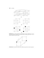
For example, in Figure 1.2 a graph G is depicted where the Bidirectional Links
restriction and the corresponding undirected graph G hold.
Reliability Restrictions Other types of restrictions are those related to reliability,
faults, and their detection.

b

c

X

Z

c

b

d

a

d

a

b

X

c

Z
d

a

c

b
b

c

Y

G = ( V, E )

b

c

Y

G = ( V, E )

FIGURE 1.2: In a network with Bidirectional Links we consider the corresponding undirected
graph.

CuuDuongThanCong.com


8

DISTRIBUTED COMPUTING ENVIRONMENTS

Detection of Faults Some systems might provide a reliable fault-detection mechanism. Following are two restrictions that describe systems that offer such capabilities
in regard to component failures:
Edge failure detection: ∀ (x, y) ∈ E, both x and y will detect whether (x, y) has
failed and, following its failure, whether it has been reactivated.
Entity failure detection: ∀x ∈ V , all in- and out-neighbors of x can detect whether

x has failed and, following its failure, whether it has recovered.
Restricted Types of Faults In some systems only some types of failures can occur:
for example, messages can be lost but not corrupted. Each situation will give rise to a
corresponding restriction. More general restrictions will describe systems or situations
where there will be no failures:
Guaranteed delivery: Any message that is sent will be received with its content
uncorrupted.
Under this restriction, protocols do not need to take into account omissions or
corruptions of messages during transmission. Even more general is the following:
Partial reliability: No failures will occur.
Under this restriction, protocols do not need to take failures into account. Note
that under Partial Reliability, failures might have occurred before the execution of a
computation. A totally fault-free system is defined by the following restriction.
Total reliability: Neither have any failures occurred nor will they occur.
Clearly, protocols developed under this restriction are not guaranteed to work
correctly if faults occur.
Topological Restrictions In general, an entity is not directly connected to all
other entities; it might still be able to communicate information to a remote entity,
using others as relayer. A system that provides this capability for all entities is characterized by the following restriction:
Connectivity: The communication topology G is strongly connected.
That is, from every vertex in G it is possible to reach every other vertex. In case
the restriction “Bidirectional Links” holds as well, connectedness will simply state
that G is connected.

CuuDuongThanCong.com


COST AND COMPLEXITY

9

Time Restrictions An interesting type of restrictions is the one relating to time.
In fact, the general model makes no assumption about delays (except that they are
finite).
Bounded communication delays: There exists a constant ⌬ such that, in the
absence of failures, the communication delay of any message on any link is at
most ⌬.
A special case of bounded delays is the following:
Unitary communication delays: In the absence of failures, the communication
delay of any message on any link is one unit of time.
The general model also makes no assumptions about the local clocks.
Synchronized clocks: All local clocks are incremented by one unit simultaneously and the interval of time between successive increments is constant.
1.4 COST AND COMPLEXITY
The computing environment we are considering is defined at an abstract level. It
models rather different systems (e.g., communication networks, distributed systems,
data networks, etc.), whose performance is determined by very distinctive factors and
costs.
The efficiency of a protocol in the model must somehow reflect the realistic costs
encountered when executed in those very different systems. In other words, we need
abstract cost measures that are general enough but still meaningful.
We will use two types of measures: the amount of communication activities and
the time required by the execution of a computation. They can be seen as measuring
costs from the system point of view (how much traffic will this computation generate
and how busy will the system be?) and from the user point of view (how long will it
take before I get the results of the computation?).
1.4.1 Amount of Communication Activities
The transmission of a message through an out-port (i.e., to an out-neighbor) is the basic
communication activity in the system; note that the transmission of a message that will
not be received because of failure still constitutes a communication activity. Thus,
to measure the amount of communication activities, the most common function used

is the number of message transmissions M, also called message cost. So in general,
given a protocol, we will measure its communication costs in terms of the number of
transmitted messages.
Other functions of interest are the entity workload Lnode = M/|V |, that is, the
number of messages per entity, and the transmission load Llink = M/|E|, that is,
the number of messages per link.

CuuDuongThanCong.com


10

DISTRIBUTED COMPUTING ENVIRONMENTS

Messages are sequences of bits; some protocols might employ messages that are
very short (e.g., O(1) bit signals), others very long (e.g., .gif files). Thus, for a more
accurate assessment of a protocol, or to compare different solutions to the same
problem that use different sizes of messages, it might be necessary to use as a cost
measure the number of transmitted bits B also called bit complexity.
In this case, we may sometimes consider the bit-defined load functions: the entity bit-workload Lbnode = B/|V |, that is, the number of bits per entity, and the
transmission bit-load Lblink = B/|E|, that is, the number of bits per link.
1.4.2 Time
An important measure of efficiency and complexity is the total execution delay, that
is, the delay between the time the first entity starts the execution of a computation and
the time the last entity terminates its execution. Note that “time” is here intended as
the one measured by an observer external to the system and will also be called real
or physical time.
In the general model there is no assumption about time except that communication delays for a single message are finite in absence of failure (Axiom 1.3.1).
In other words, communication delays are in general unpredictable. Thus, even in
the absence of failures, the total execution delay for a computation is totally unpredictable; furthermore, two distinct executions of the same protocol might experience drastically different delays. In other words, we cannot accurately measure

time.
We, however, can measure time assuming particular conditions. The measure usually employed is the ideal execution delay or ideal time complexity, T: the execution
delay experienced under the restrictions “Unitary Transmission Delays” and “Synchronized Clocks;” that is, when the system is synchronous and (in the absence of
failure) takes one unit of time for a message to arrive and to be processed.
A very different cost measure is the causal time complexity, Tcausal . It is defined
as the length of the longest chain of causally related message transmissions, over
all possible executions. Causal time is seldom used and is very difficult to measure
exactly; we will employ it only once, when dealing with synchronous computations.

1.5 AN EXAMPLE: BROADCASTING
Let us clarify the concepts expressed so far by means of an example. Consider a distributed computing system where one entity has some important information unknown
to the others and would like to share it with everybody else.
This problem is called broadcasting and it is part of a general class of problems
called information diffusion. To solve this problem means to design a set of rules that,
when executed by the entities, will lead (within finite time) to all entities knowing the
information; the solution must work regardless of which entity had the information
at the beginning.
Let E be the collection of entities and G be the communication topology.

CuuDuongThanCong.com


AN EXAMPLE: BROADCASTING

11

To simplify the discussion, we will make some additional assumptions (i.e.,
restrictions) on the system:
1. Bidirectional links; that is, we consider the undirected graph G. (see Section
1.3.2).

2. Total reliability, that is, we do not have to worry about failures.
Observe that, if G is disconnected, some entities can never receive the information,
and the broadcasting problem will be unsolvable. Thus, a restriction that (unlike the
previous two) we need to make is as follows:
3. Connectivity; that is, G is connected.
Further observe that built in the definition of the problem, there is the assumption that
only the entity with the initial information will start the broadcast. Thus, a restriction
built in the definition is as follows:
4. Unique Initiator, that is, only one entity will start.
A simple strategy for solving the broadcast problem is the following:
“if an entity knows the information, it will share it with its neighbors.”
To construct the set of rules implementing this strategy, we need to define the set S of
status values; from the statement of the problem it is clear that we need to distinguish
between the entity that initially has the information and the others: {initiator, idle} ⊆
S. The process can be started only by the initiator; let I denote the information to be
broadcasted. Here is the set of rules B(x) (the same for all entities):
1.
2.
3.
4.

initiator ×ι −→ {send(I) to N (x)}
idle × Receiving(I) −→ {Process(I); send(I) to N (x)}
initiator × Receiving(I) −→ nil
idle ×ι −→ nil

where ι denotes the spontaneous impulse event and nil denotes the null action.
Because of connectivity and total reliability, every entity will eventually receive
the information. Hence, the protocol achieves its goal and solves the broadcasting
problem.

However, there is a serious problem with these rules:
the activities generated by the protocol never terminate.
Consider, for example, the simple system with three entities x, y, z connected to each
other (see Figure 1.3). Let x be the initiator, y and z be idle, and all messages travel at
the same speed; then y and z will be forever sending messages to each other (as well
as to x).

CuuDuongThanCong.com