The effect of regional trade agreement to trade flow: evidence of trade creation and trade diversion of Asean – Japan free trade area
Bạn đang xem bản rút gọn của tài liệu. Xem và tải ngay bản đầy đủ của tài liệu tại đây (1.67 MB, 66 trang )
UNIVERSITY OF ECONOMICS
ERASMUS UNVERSITY ROTTERDAM
HO CHI MINH CITY
INSTITUTE OF SOCIAL STUDIES VIETNAM THE NETHERLANDS
VIETNAM –THE NETHERLANDS
PROGRAMME FOR M.A IN DEVELOPMENT ECONOMICS
THE EFFECT OF REGIONAL TRADE AGREEMENT TO TRADE FLOW:
EVIDENCE OF TRADE CREATION AND TRADE DIVERSION OF ASEAN –
JAPAN FREE TRADE AGREEMENT
BY
PHAM THI HIEN
MASTER OF ARTS IN DEVELOPMENT ECONOMICS
HO CHI MINH CITY, December 2016
UNIVERSITY OF ECONOMICS
INSTITUTE OF SOCIAL STUDIES
HO CHI MINH CITY
THE HAGUE VIETNAM THE NETHERLANDS
VIETNAM - NETHERLANDS
PROGRAMME FOR M.A IN DEVELOPMENT ECONOMICS
THE EFFECT OF REGIONAL TRADE AGREEMENT TO TRADE FLOW:
EVIDENCE OF TRADE CREATION AND TRADE DIVERSION OF ASEAN –
JAPAN FREE TRADE AGREEMENT
A thesis submitted in partial fulfillment of the requirements for the degree of
MASTER OF ARTS IN DEVELOPMENT ECONOMICS
By
PHAM THI HIEN
Academic Supervisor:
Prof. Dr Nguyen Trong Hoai
HO CHI MINH CITY, December 2016
DECLARATION
This is to certify that that this thesis entitled “The effect of regional trade agreement to trade flow:
Evidence of trade creation and trade diversion of ASEAN – Japan free trade agreement”, which is
submitted in fulfillment of the requirements for the degree of Master of Art in Development
Economics to Viet Nam – The Netherlands Program (VNP). The author hereby declares that she edit
this thesis individually, using only stated resources and literatures. To the best of my knowledge, my
thesis does not violate anyone’s copyright as well as any proprietary rights which are fully
acknowledge in accordance with the standard referencing practices.
HCMC, December 15th, 2016
Pham Thi Hien
ACKNOWLEDGEMENT
I am using this opportunity to express my gratitude to everyone who supports me during the master
course time.
First and foremost, I would like to sincerely thank my research supervisor, Prof. Dr. Nguyen Trong
Hoai who given to me a comprehensive guidance, great support and valuable advice during the
thesis research process. I am lucky person when every time I needed support or was in difficulties,
he has open the door to welcome me and sent to me the prompt advice.
I also would like to thank my co-supervisor Dr. Truong Dang Thuy for his enthusiastic support
and precious suggestion, which help me overcome the challenges and difficulties in doing
regression model, take me in the right direction.
I would like to express my gratitude to all lecturers of the Vietnam- Netherlands Program who
have provided the interesting lessons to build my economic knowledge during this program. In
addition, I would like to express my appreciation to the VNP academic staffs for their feedback,
cooperation during a long-period time I have learned here.
Besides, completing this work would be very difficult without the support from my best friends. I
am indebted to them for their help. Moreover, I wish to thank all my fellow master students in
VNP 21 class who share with me unforgettable memories in this program.
Last but not the least, there are also words of deep gratitude for my family who support spiritually
and encourage continuously during my thesis writing and my life in general.
Table of Contents
CHAPTER I: INTRODUCTION .................................................................................................................. 1
1.1.
Problem statement ......................................................................................................................... 1
1.2.
Research objectives ....................................................................................................................... 2
1.3.
Research questions ........................................................................................................................ 2
1.4.
Research scope .............................................................................................................................. 3
1.5.
Thesis structure ............................................................................................................................. 3
CHAPTER 2 LITERATURE REVIEW ....................................................................................................... 5
2.1.
Trade theories................................................................................................................................ 5
2.2.
Trade creation and trade diversion ................................................................................................ 5
2.2.1.
Trade creation ....................................................................................................................... 6
2.2.2.
Trade diversion ..................................................................................................................... 6
2.3.
The gravity model in international trade ....................................................................................... 8
2.3.1.
2.4.
Theoretical framework .................................................................................................................. 9
2.4.1.
2.5.
The origin of gravity model .................................................................................................. 8
Theoretical support and theoretical equation ........................................................................ 9
Empirical support for effect of FTA to ASEAN ......................................................................... 12
2.5.1.
Empirical support for effect of AFTA to intra-bloc trade flow........................................... 12
2.5.2.
Empirical support of effect of ASEAN + 1 FTAs............................................................... 13
2.6.
Zero trade data problem .............................................................................................................. 15
2.7 Chapter remark.................................................................................................................................. 17
CHAPTER 3: RESEARCH METHODOLOGY ........................................................................................ 18
3.1.
Model specification and validity testing ..................................................................................... 18
3.1.1. Model specification ....................................................................................................................... 18
3.1.2 Model validity testing .................................................................................................................... 22
3.2.
Data and data sources.................................................................................................................. 23
CHAPTER 4: RESEARCH FINDINGS AND DISCUSSION ................................................................... 25
4.1.
Descriptive statistics of variables ................................................................................................ 25
4.2.
Testing multicollinearity ............................................................................................................. 28
4.3.
Regression result ......................................................................................................................... 30
4.3.1 Comparison of estimator properties ............................................................................................... 30
4.3.2 Regression results .......................................................................................................................... 31
Chapter 5: Conclusion and policy recommendation ................................................................................... 44
5.1.
Conclusion .................................................................................................................................. 44
5.2.
Policy implication ....................................................................................................................... 45
5.3 Limitations of the study .................................................................................................................... 46
Reference .................................................................................................................................................... 47
CHAPTER I: INTRODUCTION
1.1. Problem statement
It is no doubt to saying that recently, regional trade agreements (RTA) have become a popular
widespread trend in the international economic system, especially after Doha round of GATT/
WTO. According to the definition of WTO, regional trade agreement, included free trade
agreements (FTAs) and customs unions (CUs), are the negotiations of two or more parties, in
which these participants agree to reduce their current custom barriers, such as tariffs, quotas. Since
early of the 1990s, RTAs have increased widespread. According to reports of World Trade
Organization (WTO), until February 2016, there are 625 notifications of RTAs and 419 in which
were in force. Regarding the Association of Southeast Asian Nations (ASEAN) is considered as a
successful model of regionalism and the community is step by step greatly co-operating and
integrating to the world economy. In addition, Japan, an economy was growing rapidly, involving
17% to world economic in 2005 but reduced to only 6% in 2015 (IMF, 2015). However, her
economic performance has a massive influence on the economy of the entire region. For evidence,
Japan is one of top three trading partners of ASEAN economies, especially Indonesia and the
Philippines.
Before integrating into ASEAN regional economies, Japan was playing an important role in the
regional development. In the 1970s, 25% per total import and export values of ASEAN were doing
with Japan. Moreover, with lower cost in materials and labors, ASEAN markets were attractive
destinations of capital investment flow from Japanese companies. It generated work jobs and
increased working wages, especially, with high technologies and high-trained employees, they
provided a valuable opportunity for learning and transferring in this area during the 1980s to 1990s.
The increasingly integrated business need a major opportunity to strengthen linkages between
ASEAN and Japan. That is the reason for raising a needful talk about a regional agreement.
Since 2003, the government of Japan and the 10 countries of ASEAN completely signed the
general framework of bilateral free trade agreement named ASEAN-Japan FTA (officially a
comprehensive economic partnership), hereinafter referred as AJCEP. At the end of December
2008, the last official round was finalized, an agreement signed among Asian countries, included:
Brunei Darussalam, Cambodia, Indonesia, Laos PRD, Malaysia, Myanmar, Philippines,
1
Singapore, Thailand, Vietnam and Japan has been forced, support multilateral trading by reducing
the tariff. The origin objectives of this FTA are to encourage free trade across the border in intrabloc ASEAN and Japan, strengthen Asian countries, Japan economic integration, enhance their
economic in the world market, are transparent in trading procedure and maintain sustainability in
the economic area. It seems a major opportunity for high-tech and modern industries of Japan such
as automobile, electronic, etc to enter ASEAN markets as well as encourage assembly line in
regions for Japanese firms.
Statically, after trade agreement in force, in 2013, two-way trading volume obtained $229 billion
compared with $128 billion in 2000. In this year, Japan reported 14% and 15% for import and
export value to ASEAN, Thai Land ($22.5 billion), Indonesia ($ 32.2 billion) and Malaysia ($29.6
billion) are top three Asian biggest exporters to Japan (ASEAN Statistics, 2014). The notable
products mainly exported from ASEAN to Japan are foods, manufactured goods, textiles, crude
material. Conversely, machinery and equipment transportation to gather with chemical and
advanced technology manufacturing products are important to major export from Japan to ASEAN
countries. For example, according to Japan automobile Manufacturer Association statistics in
2014, about 47% Japanese cars, 80% truck vehicles and 85% buses were consumed as final
products in ASEAN markets.
1.2. Research objectives
-
The first research purpose of this study, in general, is to examine the effect of AJCEP to
ASEAN economies in trade creation and trade diversion aspects with total export data
-
The second research objective is to examine the effect of AJCEP on sub-catalogues in
particular: food products, agricultural products, manufactured products, Machinery and
equipment of transportation and clothing and accessories and textile, fabric
1.3. Research questions
According to numerous studies before, the effect of RTAs has no guarantee positive effect to help
its member countries integrating with the global market. In many cases, RTAs actually caused
some negative effects. Therefore, this study aims to find the answers to these questions following:
-
How the trade creation and trade diversion in general total export have been caused by the
free trade agreement which was signed by AJCEP to ASEAN member countries?
2
-
How the trade creation and trade diversion have been affected by the free trade agreement
which is by AJCEP to ASEAN member countries in the five sub-catalogues: food products,
agricultural products, manufactured products, Machinery and equipment of transportation
and clothing and accessories and textile, fabric?
1.4. Research scope
To estimate the effect of AJCEP, we employ a panel data set will be collected with period from
2000 – 2015 with total 5,920 observations with included 09 ASEAN countries: Brunei Darussalam,
Cambodia, Indonesia, Lao PDR, Malaysia, Myanmar, Philippines, Singapore, Thailand, Vietnam
and 15 biggest trading partners of Japan 2015 include: The United State, China, South Korea
(Korea Rep.), Hong Kong SAR China, Australia, Saudi Arabia, The United Arab Emirates,
Russian Federation, Switzerland, New Zealand, United Kingdom, Germany, Mexico, Netherland
and Japan.
To our knowledge, there is the rapid development in investing effect of RTAs in theoretical as well
as empirical accesses. However, most of them are usually focus on general questions: whether or
not RTAs have affected to trade flow or created trade creation, trade diversion. There are two main
problems that many previous studies had.
The first problem is estimation challenges of the gravity model which solve around the
heteroscedasticity and the frequency of zero trade observations. These problems cause challenges
in concerning the most suitable estimation technique to avoid biased and un-misinterpreted result.
The second advantage is we do estimate regression model by using two sets of trade flow data.
The first data set is aggregated data is used to examine for bilateral total export flow. The second
dataset is disaggregated data is optimized to estimate the AJCEP affect to five separate subcategories: agriculture, manufacturing, chemical industry, machinery, transportation industry and
clothing and accessories and textile, fabric. By two different approaches, we can analyze impacts
of AJCEP in general and in the specific commodity in particular as well.
1.5. Thesis structure
After finishing introduction chapter, the rest of this paper is arranged as follow. Chapter 2 presents
the literature review in trade theories in international trade flow, theoretical support of gravity
model in international trade, empirical support in order so to see the development of contribution
3
studies of AJCEP effect to ASEAN member as well as Japan. In addition, this chapter reviews
empirical support of the methods to solve the popular issue of frequency of zero trade data. Chapter
3 states methodology, model construction, model estimation methods and data scope that used in
the study. Chapter 4 interprets the result and findings from the regression model. Chapter 5
summaries the thesis result and recommendation suggestion as well as limitation of the study.
4
CHAPTER 2 LITERATURE REVIEW
In this chapter, we will summary some related trade theories which are popularly used in
international trade. Then, a review of theoretical and empirical support for gravity model on trade
are added. In addition, we consider about some literature reviews about zero trade data and the
developing of estimation techniques which some previous studies used.
2.1. Trade theories
Many theories explain about the benefit that countries obtain from international trade. Among of
them is Adam Smith’s Absolute productivity advantage model. He assumed that labor and factors
of production are fixed, identical with a country and completely utilized, technology and cost of
production are constant, zero in transportation cost. Under the assumption, this law states that
country should export domestic effective product and import foreign effective product (Howse and
Trebicook, 1995). In the case occurring one country has an absolute advantage in two goods, the
comparative advantage of David Ricardo has applied. By comparing the degree of absolute
advantage or disadvantage in the production of goods, a country produces goods with lower
opportunity cost than other countries. It implies that if both countries specialize according to their
comparative advantage, they both can gain from their specialization and international trade.
However, the law of comparative advantage considers only labor is the factor of production and
trade. Heckerscher-Ohlin model explains international trade focus on the country’s resources
abundance differences between countries such as labor, capital and land. It will not meaningful if
only mention number of resources, for example, labor or land resources that country has, so the
definition of labor- and land-intensive have introduced. Therefore, a country will focus on
manufacturing products that country has an intensive factor.
2.2. Trade creation and trade diversion
Before Viner (1950), most of the studies assumed that tariffs between countries caused reducing
welfare, therefore a customs union or free trade agreement would improve welfare. He drew the
distinction between trade creation and trade diversion effects of an FTA. According to his study,
5
an FTA does not completely improve welfare. The positive or negative effects of an FTA depend
on the comparison of the magnitude of trade creation and trade diversion. If an FTA causes trade
creation more than trade diversion, it implies that this FTA has raised welfare.
2.2.1. Trade creation
When an FTA is in force, in general, we expect that with an elimination of tariff as well as trade
incentive policies, FTA will encourage trade flow that would not have existed before. It allows
member countries to concentrate and trade with their comparative advantages and get the benefits
from economic of scale. All of the trade creation cases will increase country’s national welfare.
2.2.2. Trade diversion
When a trade agreement or customs union were in force, trade flow is diverted from more efficient
exporters towards less efficient exporters because tariff between two or more countries partially
or completely removed and common tariff are still applied to rest of non-members. In reality, if
without any preference on the tariff, a country will import goods from where the goods are
provided with lowest quoted price. It is reasonable when a less cost efficient country in a union
still can export to member countries than more cost efficiency countries outside the union or FTA.
Obviously, adding tariff rate, the more cost efficiency countries will have a higher cost, leading to
higher in price, lower advantage competition. Therefore, when a union is established, the trading
flow will be shifted toward member countries, in other words, union members will get profit from
trade diversion effect, however, with non-member countries, it causes negatively economically
effect. Because without comparative in producing price but due to reducing or eliminating in tariff,
higher cost countries still can enter to market, mean the total welfare was lost in trade diversion.
Figure 1 shows the welfare effects of joining a free trade agreement. 𝐷 and 𝑆 are denoted for
domestic demand and domestic supply of a specific product 𝑋 of a country respectively.
𝑆 𝑀 and 𝑆 𝑁 are represented for exporting supply of product 𝑋 from intra-bloc member countries
and extra-blocs non-member countries.
According to Figure 1, before integrating a free trade agreement, 𝑆 𝑀 + 𝑡 and 𝑆 𝑁 + 𝑡 are denoted
for supply curves from intra-bloc and extra-bloc respectively. Assuming that non-member
countries provide product 𝑋 at a lower price than member countries do, 𝑆 𝑀 lies under 𝑆 𝑁 or 𝑆 𝑀 +
6
𝑡 lies under 𝑆 𝑁 + 𝑡 graphically. The difference between 𝐷0 − 𝑆0 is country import demand from
non-members.
After free trade agreement was formed, the supply curve 𝑆 𝑁 + 𝑡 is unchanged because tariff is
still applied to non-member countries. Meanwhile, the tariff is no longer counted to supply source
from 𝑆 𝑀 . In this case, the equilibrium price of product 𝑋 in the country will be 𝑃1 and the difference
between 𝐷1 − 𝑆1 will be import demand from member countries instead of non-members countries
as before. Considering the domestic consumer surplus is the sum of area 𝑎, 𝑏, 𝑐, 𝑑 while 𝑎 is the
surplus of domestics manufacturers falls. Regarding government, when a free trade agreement has
been in forced, government is no longer collected tax revenue because currently all importing
values comes from member countries, denoted by sum of area 𝑐. Therefore, the total effect of trade
creation caused by free trade agreement is the sum of areas 𝑏 and 𝑑.
Regarding trade diversion, the switching to the higher-cost manufacturers in intra-bloc members
instead of lower-cost from extra-bloc members is denoted for trade diversion denoted by 𝑒 area.
The total effects of free trade agreement in overall will be determined by comparing the
magnitudes of trade creation and trade diversion effects. If trade creation exceeds trade diversion
effect, welfare is enhanced due to free trade agreement. Oppositely, trade diversion effect exceeds
trade creation, it means that country welfare is decreased due to the free trade agreement.
Figure 1: Trade creation and trade diversion
7
2.3. The gravity model in international trade
2.3.1. The origin of gravity model
Gravity model has been used as a workhorse tools to analyze the international trade flow. It was
developed from the law of universal gravitation found by Isaac Newton in 1967. The law state that
every two points attract another one with a force that is in direct proportion to the product of their
masses and inverse proportion to the distance between them in square.
𝐹𝑖𝑗 = 𝐺
𝑀𝑖 𝑀𝑗
(1)
2
𝑑𝑖𝑗
Where:
𝐹𝑖𝑗 is the gravity force between two of masses
𝑀𝑖 , 𝑀𝑗 are the masses of the first and second point respectively
2
𝑑𝑖𝑗
is the distance from fist point center to the second point center in square
𝐺 is the gravitational constant with determined value equal 6.674 x 10⁻¹¹ N.(m/kg)2
The first study using gravity model which is derived from Newton’s law of gravitation to analyze
international trade flows by Tinbergen in 1962. For trade model, the bilateral trade volume
between two countries 𝑖, 𝑗 has been used to replace for the force of gravity and economic sizes
𝑌𝑖 , 𝑌𝑗 have been used to replace for the masses of 𝑀𝑖 , 𝑀𝑗 respectively. Generally, the gravity
formulation has been established in the following form:
𝛽
𝑋𝑖𝑗 = 𝐴
𝑌𝑖𝛼 𝑌𝑗
(2)
𝛾
𝑑𝑖𝑗
Where 𝛼, 𝛽, 𝛾 may take the value different to 1. They depend on the elasticity of economic sizes
of exporting country, importing country and distance respectively. In case, 𝛼 = 𝛽 = 1 and 𝛾 = 2,
it has the same formulation of Newton’s equation. Usually, economic sizes are defined as GDP,
GNP, real GDP, real GNP, income per capita or population. These essential variables represent for
supply and demand force of each country that determine country’s trade volume.
8
Regarding distance variable, it is defined by geography distance between two economics hubs or
capitals counted in land miles. Tinbergen stated that distance is not only a proxy represent for real
distance but also may stand for many other market factors which influence to trade volume such
as transportation cost, transit cost, communication exchange cost or even culture cost.
Usually, in economic regression, the simplest gravity model is estimated under OLS by taking
logarithm equation (2) and adding error term 𝜀𝑖𝑗 . The coefficient result obtained will be interpreted
as elasticity because the regression took the double log form:
𝑙𝑜𝑔 𝑋𝑖𝑗 = 𝑙𝑜𝑔 𝐴 + 𝛼𝑙𝑜𝑔 𝑌𝑖 + 𝛽 𝑙𝑜𝑔 𝑌𝑗 − 𝛾𝑙𝑜𝑔 𝐷𝑖𝑗 + 𝜀𝑖𝑗
(3)
According to the explanation above, the coefficients will be interpreted as follow:
If the economy of country 𝑖/𝑗 increases by one percent, the trade volume between two countries
will increase 𝛼/𝛽 percent respectively while other factors are held constantly. Similarly, trade
volume will reduce 𝛾 percent if the distance between two countries increases by one percent. All
in the cases, error terms 𝜀𝑖𝑗 is supposed that it is independent and normal distribution.
2.4. Theoretical framework
2.4.1. Theoretical support and theoretical equation
The first noble work in applying gravity model to international trade by Tinbergen, 1962.
However, it was still missing powerful theoretical application basic and stood outside of
mainstream due to the persistent perception of a physical gravity model more than an economic
model. The first important contribution we have to mention is the work of Anderson (1979). He
built gravity model based on Cobb-Douglas or CSE preference function under assumptions
following: each country specialize in trade completely, i.e., goods are differentiated by the origin
of a country (named Armington assumption), the preferences of consumers are homothetic and
alike across regions, no transport cost, tariff and barrier in trade. Consistent with idea that gravity
model depends on the share of expenditure of national income spent for international trade,
therefore, it can be estimated from a function of population and income. Overcome the assumption
Armington of Anderson (1979), Bergstrand (1985 and 1989) built a gravity model with
monopolistic competition created by Paul Krugman (1980). It implies that countries have
specialization in production and customer have a variety of preference, therefore, they will trade a
9
different kind of commodities from the identical country. Deardorff (1998) and Krugman (1985)
contributed the new theory to gravity model by applied literature comparative advantage of
Heckscher-Ohlin theory. Eaton and Kortum (2002) derived gravity model by using Ricardian
model, Helpman et al. (2008) added firm heterogeneity to obtain the model.
Recently, many researchers do the theoretical contribution in gravity model by importantly
concerning the usage of variables and specification. In this section, say thanks to the contribution
of Anderson and van Wincoop (2003) who developed monopolistic competition framework based
on the Armington assumption and constant elasticity of substitution (CES). Assume that customer
utility among countries are identical and homothetic, trade gravity equation was specified as
below:
𝑉𝑖𝑗 =
𝑌𝑖 𝑌𝑗
𝑌𝑤
𝑡
(𝑃 𝑖𝑗𝑃 )1−𝜎
𝑖 𝑗
(4)
Where 𝑉𝑖𝑗 is bilateral trade volume, 𝑌𝑖 , 𝑌𝑖 , 𝑌 𝑤 is income of country 𝑖, 𝑗 and global income
respectively, 𝑡𝑖𝑗 , 𝑡𝑗𝑖 are bilateral trade barrier between countries 𝑖, 𝑗, denotes all bilateral trade
resistance and assumed equally. They include distance and some binary variables such as common
border, colony, trade agreement etc. 𝜎 is the elasticity of substitution,𝑃𝑖 𝑃𝑗 , is multilateral trade
resistance and 𝑃𝑖 , 𝑃𝑗 are consumer price index of country 𝑖, 𝑗 respectively and have a function as
below:
𝑃𝑖 = [∑𝑗(𝛿𝑗 𝑝𝑗 𝑡𝑗𝑖 )1−𝜎 ]
1⁄
(1−𝜎)
(5)
And
𝑃𝑗 = [∑𝑗(𝛿𝑖 𝑝𝑖 𝑡𝑖𝑗 )1−𝜎 ]
1⁄
(1−𝜎)
(6)
Where:
𝛿𝑗 is the share of country 𝑗 in country 𝑖’s consumption, 𝑝𝑖 , 𝑝𝑗 are exporter and importer price
respectively.
10
Equation (1) and (2) show clearly that any changing in bilateral trade resistance 𝑡𝑖𝑗 in the numerator
will impact to multilateral trade resistance in the denominator and the ratio
𝑡𝑖𝑗
𝑃𝑖 𝑃 𝑗
will impact to
bilateral trade function.
To estimate border effect on international trade, they used the Non-linear Least Square (NLS)
technique. Even though they show a consistently and efficiently result that the bilateral trade cost
is depended on distance, locating landlocked, sharing the border and common language, this study
has not overcome several mistakes on its three assumptions. The first assumption is the two-way
systematization trade cost between two countries. It violates if the existence of bilateral or
multilateral trade agreement. The second violation is differences in the variety of customer
preference when they assumed that there is trade volume balance between two countries. The last
problem is on assumption about the only period of data while they missed time-varying estimator
on the regression model.
Following the methodologies of Anderson and van Wincoop (2003), Baier and Bergstrand (2007)
developed the model by extension to panel data and used time-varying fixed effect to eliminate
bias estimation caused by time-varying trade cost variables. Baldwin and Taglioni (2006)
regressed the model with the same method when choosing county-pair fixed effect to reduce
endogeneity bias caused by FTA dummy variable.
From this study, many authors use it in the different type of economic issues as the workhorse due
to its ability to correctly estimate bilateral relationship, for example, immigrant, foreign direct
investment as well as trade flow. This model has first theoretical clarification presented by
Anderson (1979) and theoretical basic later proved by Helpman and Krugman (1985), Bergstrand
(1989), and Deardorff (1998). In additional, this model was applied to many studies, can be
referred to the collective paper by Sen and Smith's (1995).
In particular, there are various empirical studies when applied this model to international trade
flow. Soloaga and Winters (2001), Antonucci and Manzocchi (2006) used this model to examine
the influence of country’s characteristics such as border, geography, distance combined with trade
agreement to trade flow.
11
2.5. Empirical support for effect of FTA to ASEAN
2.5.1. Empirical support for effect of AFTA to intra-bloc trade flow
The first FTA signed between ASEAN countries is AFTA in 1992. The origin members include
six of ten ASEAN countries: Brunei Darussalam, Malaysia, Philippines, Singapore, and Thailand.
The rest of four countries have joined in Vietnam (1995), Lao PRD (1997), Myanmar (1997) and
Cambodia (1999). Under this agreement, the tariff rate was reduced up to 99 percent for six origin
countries and 95 percent for rest of four countries by 2010. At the present, elimination of tariff
under AFTA has been completed.
At the first stage of implementation of AFTA, there are many studies predicted that effect of AFTA
to trade creation would be small. According to DeRosa (1995) estimated the effect of AFTA to
intra-bloc by using CGE, he found that effect of Most Favored Nation (MFN) has created free
trade liberalization more than effect caused by AFTA. Alternatively, Frankel and Wei (1995) used
gravity model as an ex-ante analyst to test this effect. He concluded that trade flow between
ASEAN countries was still affected by other outside important factors than ASEAN relation.
Increasingly, Endoh (1999) was as the first author introduced and applied two new definitions
trade creation and trade diversion to analysis effect of an FTA. According to his result, during
sample period 1960-1994, ASEAN countries has not absorbed the effect of AFTA in encouraging
trading flow within members. He assumed that the result implied that the trade proportion between
ASEAN countries was still small.
Since the 2000s, a development of the methodology to estimate gravity model has been raised. For
evidence, Soloaga and Winter (2001) has applied Tobit model to evaluate the effect of some major
PTAs on bilateral trade to ASEAN countries. According to his result, the coefficient of trade intrabloc was insignificant and negative. However, outside ASEAN trade were significantly
encouraged. Following next movement on methodology, Carrère (2006) applied Hausman and
Taylor method by using instrument variable and panel data, she showed a positive trade flow
within ASEAN and reducing import from rest of the world.
With the development of methodology as well as the interest on growing of FTA of ASEAN, a
number of studies focused on their impact on ASEAN countries economies have been grown
moderately. Elliot and Ikemoto (2004) applied gravity model to examine the effect of AFTA on
12
trade creation and trade diversion. Matching with some previous studies, they found that ASEAN
countries have been gained benefit from AFTA both create on and diversion when coefficients
effect were positive and significant. With the same result, Bunn et al. (2009) employed two kinds
of FTA dummies, first is FTA dummies which take value one if two member countries of AFTA
from 1992 and 0 otherwise. The second dummy was AFTA dummies multiplied to time trend to
capture the possessive tariff elimination under AFTA. He found that AFTA has positively affected
to trade throughout collected data and proposed that the including of unobserved explanation
variables to estimation model carefully to absorbed trend in trade was needful.
Among studies about AFTA effect, some of them focused on tariff reduction progress under an
agreement on the common effective preferential tariff scheme (CEPT). Pelkmans-Balaoing (2007)
used a short-time sample data from 2001-2003 in aggregated and disaggregated trade data flow to
estimate AFTA effect to ASEAN member countries. Although limited on data, they focused on
the effectiveness of preference margin on trade carefully. The results showed that AFTA has no or
slight effect to intra-bloc trade, in essence, meanwhile creating a positive effect on some range of
products in which preference margin is more than 25 percent. Moreover, his result implied that the
cost of applying AFTA would be higher than benefit obtaining from AFTA when the difference
of tariff of Most Favored Nation (MFN) and AFTA is slight. Okabe and Urata (2013) investigated
the effect of tariff elimination under CEPT through 52 products of ASEAN member countries in
the period 1980-2010. They found that AFTA has created trade creation effect. However, the
magnitude of effect to new members such as Cambodia, Lao, Vietnam was pure small. This result
could be explained by the small share of new members as well as a subsequent schedule of tariff
reduction. Moreover, the impact to trade flow is not extremely strong. From these arguments can
conclude that tariff reduction is not an essential measurement to promote regional trade flow. To
promote ASEAN trade flow as well as increase welfare for all member countries, other factors
such as trade facilitation, eliminating non-tariff barriers (NTMs), equalizing rules of origin (RoO)
as well as enhancing AFTA utilization should be considered.
2.5.2. Empirical support of effect of ASEAN + 1 FTAs
A definition has been raised in many recent studies about free trade agreements (FTAs) and
regional free trade agreements (RTAs) are “noodle bowl effect: stumbling or building block?”.
This definition is completely correct with ASEAN’s trade agreements status. The reason for that
13
is to gather with General Agreement on Tariff and Trade (GATT), World Trade Organization
(WTO), ASEAN has multilateral FTAs with six major economy countries named: Australia, New
Zealand, China, Japan, Korea and India since the middle of the 2000s. In addition, a remarkable
number of bilateral FTAs has been signed and effected between these countries and ASEAN
members, such as Japan has bilateral FTAs with Indonesia, Malaysia, Philippine, Singapore,
Thailand, Vietnam; India has bilateral FTAs with Malaysia, Singapore; China has formed bilateral
FTAs with Singapore, Thailand…
Following integration trend in international trade when FTAs related to ASEAN in force, a number
of ex-ante and studies has been made to estimate the effect of these FTAs caused to ASEAN.
Estrada et al. (2011) used simulation analyst CGE model to compare the effect to welfare of
member countries caused by ASEAN + China, ASEAN + Japan and ASEAN + Korea with current
ASEAN + 1 FTAs. He found that these FTAs has caused positive expectation and fascination to
members China, Korea and Japan. Using same as econometric technique CGE model to predict
the impact of ASEAN + 1 FTAs, Sheng et al. (2012) estimated gravity model period from 19802008, he predicted that ASEAN-China (ACFTA) has caused massive impact to trading flow.
Especially, it affected to adjacent production linkage internationally and positive impact spreading
among ASEAN countries. Bano et al. (2013) analyzed trade effect caused by ASEAN-AustraliaNew Zealand (AANZFTA) with data after 1980 with positive effect to trade across ASEAN
countries and New Zealand, Australia was proposed. Chandran (2012) worked with India-ASEAN
FTA (AIFTA) focusing on fishery division, he quoted that the FTA has improved trade by tariff
reduction, particularly low-developed countries. Okabe (2015) used CGE model to forecast the
effect of current ASEAN + 1 FTAs include ACFTA, AKFTA and AJCEP. She found that trade
creation has been caused by ACFTA, AKFTA in two sub-categories: industrial supplies and capital
goods. Misa (2015) used the sample data from 2002 to 2012 and gravity model to estimate the
effect of ASEAN +1 FTAs. They found that ASEAN-China FTA and ASEAN-Korea FTA has
cause positive trade creation in industrial supplies and capital goods among member countries. In
addition, ASEAN-China also facilitates consumption goods. In contrary, ASEAN-Japan has not
revealed the impact on many cases.
In general, the impact of AJCEP appeared limitedly at the moment of ex-post analysis. Meanwhile,
most of the studies about AJCEP show a negative or unclear effects. The reason could be used to
14
explain this result was tariff reduction schedule and RoO certification while other former FTAs
have been implicated in the longer time. That is one of the reason encourage us re-estimate the
effect of AJCEP to ASEAN members by using by the ex-post analyst.
2.6. Zero trade data problem
Zero trade flow between a given pair of countries is a problem has been widely discussed. Because
the traditional way usually used to estimate gravity model is taking logarithms leading to drop out
zero value to the data set. However, zero data is not completely mean non-trade between two
countries. It may imply the trade volume with very small flows or even missing or loss when
reporting process in many cases.
In reality, several alternative zero approaches have been discussed. The first method is truncate
zeros data and still estimate log-linear by OLS. By this method, zero trade data will be completely
deleted from the matrix. The second solution is the censoring method by substituting a small
constant volume, for example, one dollar before taking logarithms trade value when estimating
gravity model in level. However, these methods can lead to inconsistent estimates and distort the
significant result Burger et al., 2009, Gomez-Herrera, 2013. Moreover, according to Flowerdew
and Aitkin (1982) indicate that the result is sensitive when replacing ad hoc zero data for small
value is not guaranteed for an expected regression result, can-not be avoided inconsistent
estimation. Eichengreen and Irwin (1998), Heckman (1979), Helpman et al., (2008) debated that
in case zero data do not follow the random distribution, deleting zero data from trade matrix can
lead to loss valuable information and create bias results.
With the same result, Linder and Groot posit that applying truncation or censor method when
dealing with zero data may lead to misunderstanding bilateral trade patterns. Because maybe due
to far distance, low level in GDP or non-linkage in culture or historical, non-profitable in trade,
firms make decision reducing trade or non-trading, then we eliminate zero data will cause
underestimating coefficients. Therefore, there is an attention on finding an appropriate technique
to deal with zero data recently.
Some early studies have used Tobit model to deal with it, for example, Rose (2004), Andersen and
Marcouiller (2002). With Tobit model, data will be fitted when data is observed in some range,
involving rounding part of the observation to zero and rounding up the zero trade flow which below
15
positive value. However, Linder and Groot, 2006 debated the appropriateness when using Tobit
model to fit data when zero trade. According to their argument, zero trade flow can-not be censored
at zero because desired bilateral trade can-not be negative except one or both countries in a pair
have GDP equal 0, however, it is not real. In addition, they indicated that censoring at positive
value is also not appropriated, even 1$ only. Because in UNCOMTRADE trade flow database,
sometimes zero trade are caused by actual economic decision situation. In this case, taking care of
zero trade is needless. Therefore, subject to measurement errors, this method will high influence
to regression results, Frankel (1997).
Recently, Head and Mayer (2013) has proposed new approach when dealing with a set of data with
25 percent by gravity model, based on Eaton and Kortum (2001), named EK Tobit model. By this
method, they will replace all zero trade data from country 𝑖 to all destination country 𝑗by minimum
level of trade data recorded. This method has two advantages. First, without any criteria, we will
easily collect minimum trade value which used to replace. Second, easily estimate the model by
using command 𝑖𝑛𝑡𝑟𝑒𝑔 in Stata.
Another attention new method was developed by Santo Silva and Tenreyro (2006; 2011) is Poison
Pseudo Maximum Likelihood (PPML) to deal with logarithm transformation and zero trade flow
data. They deal with a set of data with a share of zero trade at 62 percent. According to their
argument, PPML estimation will fix the problem by regressing model in the level instead of taking
logarithms. By this method, it will address observed heterogeneity, provide the instinctive way to
estimate the model with zero trade because we no need to do log-linearized and lowest bias among
other estimators. However, Martin and Pham (2008), Burger et al., 2009, argued controversially
that PPML method has some limitation, especially do not take account unobserved heterogeneity.
More recently, Head and Mayer (2014) proposed new method name Multinomial Pseudo
Maximum Likelihood (MPML). In this method, dependent variable will be
𝑌𝑖𝑗
𝑌𝑗
as a market share
variable and estimate by Stata command 𝑝𝑜𝑖𝑠𝑜𝑛 along with fixed effect.
Another method proposed by Burger et al., (2009) to take care unobserved heterogeneity are
Negative Binomial Pseudo Maximum Likelihood (NBPML) and Zero-inflated Pseudo Maximum
Likelihood (ZIPML). However, they posit that this method is not well-suited for the cases a
16
number of zero trade data predicted by the model is lower than a number of zero trade data flow
observed.
In sum, according to listed review, each method has own pros and cons and the best method has
not yet to be defined, remain in debate and are not an unclear decision. However, in this paper,
data is updated for time period recently from 2000-2015, the trade zero data were recorded at 15
percentage and concentrate on data of Cambodia and Brunei. In 2015, the total export value of
Cambodia and Brunei to the rest of the world were reported at 0.42 percent and 0.34 percent per
total export value of the countries in this sample. Therefore, we chose the simplest estimation
method in case of present zero trade is dropping them out the data.
2.7 Chapter remark
The application of gravity model to explain the trade relations in the international trade become
very popular. It could be proved by a rigorous development in related theoretical support as well
as empirical contribution. However, in spite of the popularity, it remains some questions about the
adequacy of model specification and proper estimation technique which should be used for a
consistent estimation to deal with the frequency of zero trade data, occurring when about 50%
trade data have found in zero. Each method has own pros and cons and had not be defined.
Therefore, within this study with about 15% zero trade data, we will use the simple technique to
tackle with it. However, our analyst will be wider by comprising some regression techniques in
order to obtain suitable estimator for our database.
17
CHAPTER 3: RESEARCH METHODOLOGY
In this chapter, we will diagnose the gravity model applied to international trade from
multiplicative to logarithmic form. We did it by adding variables which effect to bilateral trade to
gravity model to investigate the impact of AJCEP to ASEAN as well as Japan. Then, we process
by using a variety of estimation techniques such as OLS, Fixed effect model (FEM), Random
effect model (REM), Hausman-Taylor estimator. In addition, an overview of data scope and data
sources are also mentioned in this Chapter.
3.1. Model specification and validity testing
3.1.1. Model specification
Starting with the multiplicative equation of gravity model in international trade:
𝛽
𝛽
𝛽
𝛽
𝛽
𝛽
𝑋𝑖𝑗 = 𝛽0 𝐺𝐷𝑃𝑖 1 𝐺𝐷𝑃𝑗 2 𝑃𝑂𝑃𝑖 3 𝑃𝑂𝑃𝑗 4 𝐷𝐼𝑆𝑇𝑖𝑗 5 𝐹𝑖𝑗 6 𝑢𝑖𝑗𝑡 (7)
Following to the gravity model of international trade, the function of the total bilateral volume of
export of a couple of countries 𝑋𝑖𝑗 is included their GDPs, population, distance and 𝐹𝑖𝑗 denotes a
set of dummy elements which encouraging or discouraging bilateral trade flow included Border,
Language, Colony, Land-lockedness, Free trade agreement.
For estimation target as well as time dimension plus, we change model (7) into log-liner format
which is given as below:
𝑙𝑛𝑋𝑖𝑗𝑡 = 𝛽0 + 𝛽1 𝑙𝑛𝐺𝐷𝑃𝑖𝑡 + 𝛽2 𝑙𝑛𝐺𝐷𝑃𝑗𝑡 + 𝛽3 𝑙𝑛𝑃𝑂𝑃𝑖𝑡 + 𝛽4 𝑃𝑂𝑃𝑗𝑡 + 𝛽5 𝑙𝑛𝐷𝐼𝑆𝑇𝑖𝑗 + 𝛽6 𝐿𝐴𝑁𝐺𝑖𝑗 +
𝛽7 𝐵𝑂𝑅𝑖𝑗 + 𝛽8 𝐿𝐿𝑂𝐶𝐾𝑖𝑗 + 𝛽9 𝐶𝑂𝐿𝑖𝑗 + 𝛽10 𝐹𝑇𝐴𝑖𝑗𝑡 + 𝑢𝑖𝑗𝑡
(8)
Where:
Dependent variable
Trade flow (𝑋𝑖𝑗𝑡 ): in the gravity model, we employ variable trade flow by export volume from
exporting country 𝑖 to importing country 𝑗 at time t at current US$.
Independent variables
Gross domestic products GDP (𝑖𝑡, 𝑗𝑡)
18
GPD at current US$ is the first independent variables which collected from the database of World
trade organization WTO. This variable denoted for total value within a certain time 𝑡at current
US$ of all final goods and services produced in a country. In gravity model, it includes 𝐺𝐷𝑃𝑖𝑡 and
𝐺𝐷𝑃𝑗𝑡 which consider 𝑖 is exporting country and 𝑗 is importing country. According to utility theory,
when the income and output of a country increase, it will increase consumer demand for goods
and service, leading to increasing production and export. Nellis and Parker (2004), 𝐺𝐷𝑃 presents
for country’s income and purchasing power, therefore, GDP will have the positive sign with total
import plus export volume. However, Basat (2002) indicated that positive relation only with
middle development countries, there is no evidence for low and high development countries.
Population POP (𝑖𝑡, 𝑗𝑡):
The population is the second independent variable, divided to two population variables,
𝑃𝑂𝑃𝑖𝑡 denoted for the population of exporting country 𝑖 and 𝑃𝑂𝑃𝑗𝑡 will denote for the population
of importing country 𝑗 at time 𝑡 at million unit. It is forecasted that which a country with a larger
population, they will have larger demand on import as well as export. However, Aiken (1973)
proposed that in the countries with a large population, the ratio of domestic market demand to the
foreign market demand will higher than one, therefore, therefore, the smaller population countries
will have more export volume. Therefore, according to Oguledo and Macphee (1994) 𝛽3 , 𝛽4 are
expected negative or positive signs relying on each country’s integration level.
Weighted distance DIST (𝐷𝐼𝑆𝑇𝑖𝑗 )
Weighted distance is the third independent variable is calculated by Mayer and Zignago (2005),
based on inspired idea of Head and Mayer (2002) is calculating geographic distance between two
countries 𝑖 and 𝑗 by biggest cities distance, inner cities distance being weighted by population ratio
of the city to the total country’s population.
The reason for using this method instead of simple geodesic distance which calculated by using
longitudes and latitudes is to avoid over or underestimate the effect of the border. Taking an
example of trading volume between Vietnam and China, one of the factor include to trade volume
is the comparison of domestics transportation cost inside China internally and international
transportation cost between China-Vietnam and population in these cities. The general function
was developed by Head and Mayer (2002) to calculate the weighted-distance from country 𝑖 to
country 𝑗 is:
19