J k lindsey applying generalized linear models
Bạn đang xem bản rút gọn của tài liệu. Xem và tải ngay bản đầy đủ của tài liệu tại đây (1.32 MB, 272 trang )
Applying Generalized
Linear Models
James K. Lindsey
Springer
Preface
Generalized linear models provide a unified approach to many of the most
common statistical procedures used in applied statistics. They have applications in disciplines as widely varied as agriculture, demography, ecology, economics, education, engineering, environmental studies and pollution, geography, geology, history, medicine, political science, psychology,
and sociology, all of which are represented in this text.
In the years since the term was first introduced by Nelder and Wedderburn in 1972, generalized linear models have slowly become well known and
widely used. Nevertheless, introductory statistics textbooks, and courses,
still most often concentrate on the normal linear model, just as they did in
the 1950s, as if nothing had happened in statistics in between. For students
who will only receive one statistics course in their career, this is especially
disastrous, because they will have a very restricted view of the possible
utility of statistics in their chosen field of work. The present text, being
fairly advanced, is not meant to fill that gap; see, rather, Lindsey (1995a).
Thus, throughout much of the history of statistics, statistical modelling
centred around this normal linear model. Books on this subject abound.
More recently, log linear and logistic models for discrete, categorical data
have become common under the impetus of applications in the social sciences and medicine. A third area, models for survival data, also became a
growth industry, although not always so closely related to generalized linear
models. In contrast, relatively few books on generalized linear models, as
such, are available. Perhaps the explanation is that normal and discrete, as
well as survival, data continue to be the major fields of application. Thus,
many students, even in relatively advanced statistics courses, do not have
vi
an overview whereby they can see that these three areas, linear normal,
categorical, and survival models, have much in common. Filling this gap is
one goal of this book.
The introduction of the idea of generalized linear models in the early
1970s had a major impact on the way applied statistics is carried out. In the
beginning, their use was primarily restricted to fairly advanced statisticians
because the only explanatory material and software available were addressed
to them. Anyone who used the first versions of GLIM will never forget
the manual which began with pages of statistical formulae, before actually
showing what the program was meant to do or how to use it.
One had to wait up to twenty years for generalized linear modelling
procedures to be made more widely available in computer packages such
as Genstat, Lisp-Stat, R, S-Plus, or SAS. Ironically, this is at a time when
such an approach is decidedly outdated, not in the sense that it is no longer
useful, but in its limiting restrictions as compared to what statistical models
are needed and possible with modern computing power. What are now
required, and feasible, are nonlinear models with dependence structures
among observations. However, a unified approach to such models is only
slowly developing and the accompanying software has yet to be put forth.
The reader will find some hints in the last chapter of this book.
One of the most important accomplishments of generalized linear models
has been to promote the central role of the likelihood function in inference.
Many statistical techniques are proposed in the journals every year without
the user being able to judge which are really suitable for a given data
set. Most ad hoc measures, such as mean squared error, distinctly favour
the symmetry and constant variance of the normal distribution. However,
statistical models, which by definition provide a means of calculating the
probability of the observed data, can be directly compared and judged:
a model is preferable, or more likely, if it makes the observed data more
probable (Lindsey, 1996b). This direct likelihood inference approach will be
used throughout, although some aspects of competing methods are outlined
in an appendix.
A number of central themes run through the book:
• the vast majority of statistical problems can be formulated, in a unified way, as regression models;
• any statistical models, for the same data, can be compared (whether
nested or not) directly through the likelihood function, perhaps, with
the aid of some model selection criterion such as the AIC;
• almost all phenomena are dynamic (stochastic) processes and, with
modern computing power, appropriate models should be constructed;
• many so called “semi-” and “nonparametric” models (although not
nonparametric inference procedures) are ordinary (often saturated)
vii
generalized linear models involving factor variables; for inferences, one
must condition on the observed data, as with the likelihood function.
Several important and well-known books on generalized linear models are
available (Aitkin et al., 1989; McCullagh and Nelder, 1989; Dobson, 1990;
Fahrmeir and Tutz, 1994); the present book is intended to be complementary to them.
For this text, the reader is assumed to have knowledge of basic statistical
principles, whether from a Bayesian, frequentist, or direct likelihood point
of view, being familiar at least with the analysis of the simpler normal linear
models, regression and ANOVA. The last chapter requires a considerably
higher level of sophistication than the others.
This is a book about statistical modelling, not statistical inference. The
idea is to show the unity of many of the commonly used models. In such
a text, space is not available to provide complete detailed coverage of each
specific area, whether categorical data, survival, or classical linear models.
The reader will not become an expert in time series or spatial analysis
by reading this book! The intention is rather to provide a taste of these
different areas, and of their unity. Some of the most important specialized
books available in each of these fields are indicated at the end of each
chapter.
For the examples, every effort has been made to provide as much background information as possible. However, because they come from such a
wide variety of fields, it is not feasible in most cases to develop prior theoretical models to which confirmatory methods, such as testing, could be
applied. Instead, analyses primarily concern exploratory inference involving
model selection, as is typical of practice in most areas of applied statistics.
In this way, the reader will be able to discover many direct comparisons
of the application of the various members of the generalized linear model
family.
Chapter 1 introduces the generalized linear model in some detail. The
necessary background in inference procedures is relegated to Appendices A
and B, which are oriented towards the unifying role of the likelihood function and include details on the appropriate diagnostics for model checking.
Simple log linear and logistic models are used, in Chapter 2, to introduce
the first major application of generalized linear models. These log linear
models are shown, in turn, in Chapter 3, to encompass generalized linear
models as a special case, so that we come full circle. More general regression techniques are developed, through applications to growth curves, in
Chapter 4. In Chapter 5, some methods of handling dependent data are described through the application of conditional regression models to longitudinal data. Another major area of application of generalized linear models
is to survival, and duration, data, covered in Chapters 6 and 7, followed by
spatial models in Chapter 8. Normal linear models are briefly reviewed in
Chapter 9, with special reference to model checking by comparing them to
viii
nonlinear and non-normal models. (Experienced statisticians may consider
this chapter to be simpler than the the others; in fact, this only reflects
their greater familiarity with the subject.) Finally, the unifying methods
of dynamic generalized linear models for dependent data are presented in
Chapter 10, the most difficult in the text.
The two-dimensional plots were drawn with MultiPlot, for which I thank
Alan Baxter, and the three-dimensional ones with Maple. I would also like
to thank all of the contributors of data sets; they are individually cited with
each table.
Students in the masters program in biostatistics at Limburgs University
have provided many comments and suggestions throughout the years that
I have taught this course there. Special thanks go to all the members of the
Department of Statistics and Measurement Theory at Groningen University
who created the environment for an enjoyable and profitable stay as Visiting
Professor while I prepared the first draft of this text. Philippe Lambert,
Patrick Lindsey, and four referees provided useful comments that helped to
improve the text.
Diepenbeek
J.K.L.
December, 1996
Contents
Preface
1 Generalized Linear Modelling
1.1 Statistical Modelling . . . . . . . . . . . . . . . . .
1.1.1 A Motivating Example . . . . . . . . . . . .
1.1.2 History . . . . . . . . . . . . . . . . . . . .
1.1.3 Data Generating Mechanisms and Models .
1.1.4 Distributions . . . . . . . . . . . . . . . . .
1.1.5 Regression Models . . . . . . . . . . . . . .
1.2 Exponential Dispersion Models . . . . . . . . . . .
1.2.1 Exponential Family . . . . . . . . . . . . . .
1.2.2 Exponential Dispersion Family . . . . . . .
1.2.3 Mean and Variance . . . . . . . . . . . . . .
1.3 Linear Structure . . . . . . . . . . . . . . . . . . .
1.3.1 Possible Models . . . . . . . . . . . . . . . .
1.3.2 Notation for Model Formulae . . . . . . . .
1.3.3 Aliasing . . . . . . . . . . . . . . . . . . . .
1.4 Three Components of a GLM . . . . . . . . . . . .
1.4.1 Response Distribution or “Error Structure”
1.4.2 Linear Predictor . . . . . . . . . . . . . . .
1.4.3 Link Function . . . . . . . . . . . . . . . . .
1.5 Possible Models . . . . . . . . . . . . . . . . . . . .
1.5.1 Standard Models . . . . . . . . . . . . . . .
1.5.2 Extensions . . . . . . . . . . . . . . . . . .
v
.
.
.
.
.
.
.
.
.
.
.
.
.
.
.
.
.
.
.
.
.
.
.
.
.
.
.
.
.
.
.
.
.
.
.
.
.
.
.
.
.
.
.
.
.
.
.
.
.
.
.
.
.
.
.
.
.
.
.
.
.
.
.
.
.
.
.
.
.
.
.
.
.
.
.
.
.
.
.
.
.
.
.
.
.
.
.
.
.
.
.
.
.
.
.
.
.
.
.
.
.
.
.
.
.
1
1
1
4
6
6
8
9
10
11
11
13
14
15
16
18
18
18
18
20
20
21
x
Contents
1.6
1.7
Inference . . . . . . . . . . . . . . . . . . . . . . . . . . . . .
Exercises . . . . . . . . . . . . . . . . . . . . . . . . . . . .
2 Discrete Data
2.1 Log Linear Models . . . . . . .
2.1.1 Simple Models . . . . .
2.1.2 Poisson Representation
2.2 Models of Change . . . . . . . .
2.2.1 Mover–Stayer Model . .
2.2.2 Symmetry . . . . . . . .
2.2.3 Diagonal Symmetry . .
2.2.4 Long-term Dependence .
2.2.5 Explanatory Variables .
2.3 Overdispersion . . . . . . . . .
2.3.1 Heterogeneity Factor . .
2.3.2 Random Effects . . . . .
2.3.3 Rasch Model . . . . . .
2.4 Exercises . . . . . . . . . . . .
23
25
.
.
.
.
.
.
.
.
.
.
.
.
.
.
.
.
.
.
.
.
.
.
.
.
.
.
.
.
.
.
.
.
.
.
.
.
.
.
.
.
.
.
.
.
.
.
.
.
.
.
.
.
.
.
.
.
.
.
.
.
.
.
.
.
.
.
.
.
.
.
.
.
.
.
.
.
.
.
.
.
.
.
.
.
27
27
28
30
31
32
33
35
36
36
37
38
38
39
44
3 Fitting and Comparing Probability Distributions
3.1 Fitting Distributions . . . . . . . . . . . . . . . . .
3.1.1 Poisson Regression Models . . . . . . . . .
3.1.2 Exponential Family . . . . . . . . . . . . . .
3.2 Setting Up the Model . . . . . . . . . . . . . . . . .
3.2.1 Likelihood Function for Grouped Data . . .
3.2.2 Comparing Models . . . . . . . . . . . . . .
3.3 Special Cases . . . . . . . . . . . . . . . . . . . . .
3.3.1 Truncated Distributions . . . . . . . . . . .
3.3.2 Overdispersion . . . . . . . . . . . . . . . .
3.3.3 Mixture Distributions . . . . . . . . . . . .
3.3.4 Multivariate Distributions . . . . . . . . . .
3.4 Exercises . . . . . . . . . . . . . . . . . . . . . . .
.
.
.
.
.
.
.
.
.
.
.
.
.
.
.
.
.
.
.
.
.
.
.
.
.
.
.
.
.
.
.
.
.
.
.
.
.
.
.
.
.
.
.
.
.
.
.
.
.
.
.
.
.
.
.
.
.
.
.
.
49
49
49
52
54
54
55
57
57
58
60
63
64
4 Growth Curves
4.1 Exponential Growth Curves .
4.1.1 Continuous Response
4.1.2 Count Data . . . . . .
4.2 Logistic Growth Curve . . . .
4.3 Gomperz Growth Curve . . .
4.4 More Complex Models . . . .
4.5 Exercises . . . . . . . . . . .
.
.
.
.
.
.
.
.
.
.
.
.
.
.
.
.
.
.
.
.
.
.
.
.
.
.
.
.
.
.
.
.
.
.
.
69
70
70
71
72
74
76
82
5 Time Series
5.1 Poisson Processes . . . . . . . . . . . . . . . . . . . . . . . .
5.1.1 Point Processes . . . . . . . . . . . . . . . . . . . . .
87
88
88
.
.
.
.
.
.
.
.
.
.
.
.
.
.
.
.
.
.
.
.
.
.
.
.
.
.
.
.
.
.
.
.
.
.
.
.
.
.
.
.
.
.
.
.
.
.
.
.
.
.
.
.
.
.
.
.
.
.
.
.
.
.
.
.
.
.
.
.
.
.
.
.
.
.
.
.
.
.
.
.
.
.
.
.
.
.
.
.
.
.
.
.
.
.
.
.
.
.
.
.
.
.
.
.
.
.
.
.
.
.
.
.
.
.
.
.
.
.
.
.
.
.
.
.
.
.
.
.
.
.
.
.
.
.
.
.
.
.
.
.
.
.
.
.
.
.
.
.
.
.
.
.
.
.
.
.
.
.
.
.
.
.
.
.
.
.
.
.
.
.
.
.
.
.
.
.
.
.
.
.
.
.
.
.
.
.
.
.
.
.
.
.
.
.
.
.
.
.
.
.
.
.
.
.
.
.
.
.
.
.
.
.
.
.
.
.
.
.
.
.
.
.
.
.
Contents
.
.
.
.
.
.
.
.
.
.
.
.
.
.
.
.
.
.
.
.
.
.
.
.
.
.
.
.
.
.
.
.
.
.
.
.
.
.
.
.
.
.
.
.
.
.
.
.
.
.
.
.
.
.
.
.
.
.
.
.
.
.
.
.
.
.
.
.
.
.
.
.
.
.
.
.
.
.
.
.
.
.
.
.
.
.
.
.
.
.
. 88
. 88
. 90
. 91
. 93
. 96
. 101
. 102
. 103
6 Survival Data
6.1 General Concepts . . . . . . . . . . . . . .
6.1.1 Skewed Distributions . . . . . . . .
6.1.2 Censoring . . . . . . . . . . . . . .
6.1.3 Probability Functions . . . . . . .
6.2 “Nonparametric” Estimation . . . . . . .
6.3 Parametric Models . . . . . . . . . . . . .
6.3.1 Proportional Hazards Models . . .
6.3.2 Poisson Representation . . . . . .
6.3.3 Exponential Distribution . . . . . .
6.3.4 Weibull Distribution . . . . . . . .
6.4 “Semiparametric” Models . . . . . . . . .
6.4.1 Piecewise Exponential Distribution
6.4.2 Cox Model . . . . . . . . . . . . .
6.5 Exercises . . . . . . . . . . . . . . . . . .
.
.
.
.
.
.
.
.
.
.
.
.
.
.
.
.
.
.
.
.
.
.
.
.
.
.
.
.
.
.
.
.
.
.
.
.
.
.
.
.
.
.
.
.
.
.
.
.
.
.
.
.
.
.
.
.
.
.
.
.
.
.
.
.
.
.
.
.
.
.
.
.
.
.
.
.
.
.
.
.
.
.
.
.
.
.
.
.
.
.
.
.
.
.
.
.
.
.
.
.
.
.
.
.
.
.
.
.
.
.
.
.
.
.
.
.
.
.
.
.
.
.
.
.
.
.
.
.
.
.
.
.
.
.
.
.
.
.
.
.
109
109
109
109
111
111
113
113
113
114
115
116
116
116
117
7 Event Histories
7.1 Event Histories and Survival Distributions
7.2 Counting Processes . . . . . . . . . . . . .
7.3 Modelling Event Histories . . . . . . . . .
7.3.1 Censoring . . . . . . . . . . . . . .
7.3.2 Time Dependence . . . . . . . . . .
7.4 Generalizations . . . . . . . . . . . . . . .
7.4.1 Geometric Process . . . . . . . . .
7.4.2 Gamma Process . . . . . . . . . .
7.5 Exercises . . . . . . . . . . . . . . . . . .
.
.
.
.
.
.
.
.
.
.
.
.
.
.
.
.
.
.
.
.
.
.
.
.
.
.
.
.
.
.
.
.
.
.
.
.
.
.
.
.
.
.
.
.
.
.
.
.
.
.
.
.
.
.
.
.
.
.
.
.
.
.
.
.
.
.
.
.
.
.
.
.
.
.
.
.
.
.
.
.
.
.
.
.
.
.
.
.
.
.
121
122
123
123
124
124
127
128
132
136
8 Spatial Data
8.1 Spatial Interaction . . . . . . .
8.1.1 Directional Dependence
8.1.2 Clustering . . . . . . . .
8.1.3 One Cluster Centre . . .
8.1.4 Association . . . . . . .
8.2 Spatial Patterns . . . . . . . . .
8.2.1 Response Contours . . .
.
.
.
.
.
.
.
.
.
.
.
.
.
.
.
.
.
.
.
.
.
.
.
.
.
.
.
.
.
.
.
.
.
.
.
.
.
.
.
.
.
.
.
.
.
.
.
.
.
.
.
.
.
.
.
.
.
.
.
.
.
.
.
.
.
.
.
.
.
.
141
141
141
145
147
147
149
149
5.2
5.3
5.4
5.1.2 Homogeneous Processes . .
5.1.3 Nonhomogeneous Processes
5.1.4 Birth Processes . . . . . . .
Markov Processes . . . . . . . . . .
5.2.1 Autoregression . . . . . . .
5.2.2 Other Distributions . . . . .
5.2.3 Markov Chains . . . . . . .
Repeated Measurements . . . . . .
Exercises . . . . . . . . . . . . . .
.
.
.
.
.
.
.
.
.
.
.
.
.
.
.
.
.
.
.
.
.
.
.
.
.
.
.
.
.
.
.
.
.
.
.
.
.
.
.
.
.
.
.
.
.
.
.
.
.
.
.
.
.
.
.
xi
.
.
.
.
.
.
.
.
.
.
.
.
.
.
xii
Contents
8.3
8.2.2 Distribution About a Point . . . . . . . . . . . . . . 152
Exercises . . . . . . . . . . . . . . . . . . . . . . . . . . . . 154
9 Normal Models
9.1 Linear Regression . . . . .
9.2 Analysis of Variance . . .
9.3 Nonlinear Regression . . .
9.3.1 Empirical Models .
9.3.2 Theoretical Models
9.4 Exercises . . . . . . . . .
.
.
.
.
.
.
.
.
.
.
.
.
.
.
.
.
.
.
.
.
.
.
.
.
.
.
.
.
.
.
.
.
.
.
.
.
.
.
.
.
.
.
.
.
.
.
.
.
.
.
.
.
.
.
.
.
.
.
.
.
.
.
.
.
.
.
.
.
.
.
.
.
.
.
.
.
.
.
.
.
.
.
.
.
159
160
161
164
164
165
167
10 Dynamic Models
10.1 Dynamic Generalized Linear Models
10.1.1 Components of the Model . .
10.1.2 Special Cases . . . . . . . . .
10.1.3 Filtering and Prediction . . .
10.2 Normal Models . . . . . . . . . . . .
10.2.1 Linear Models . . . . . . . . .
10.2.2 Nonlinear Curves . . . . . . .
10.3 Count Data . . . . . . . . . . . . . .
10.4 Positive Response Data . . . . . . .
10.5 Continuous Time Nonlinear Models .
.
.
.
.
.
.
.
.
.
.
.
.
.
.
.
.
.
.
.
.
.
.
.
.
.
.
.
.
.
.
.
.
.
.
.
.
.
.
.
.
.
.
.
.
.
.
.
.
.
.
.
.
.
.
.
.
.
.
.
.
.
.
.
.
.
.
.
.
.
.
.
.
.
.
.
.
.
.
.
.
.
.
.
.
.
.
.
.
.
.
.
.
.
.
.
.
.
.
.
.
.
.
.
.
.
.
.
.
.
.
.
.
.
.
.
.
.
.
.
.
.
.
.
.
.
.
.
.
.
.
173
173
173
174
174
175
176
181
186
189
191
A Inference
A.1 Direct Likelihood Inference . . . . . . . . .
A.1.1 Likelihood Function . . . . . . . . .
A.1.2 Maximum Likelihood Estimate . . .
A.1.3 Parameter Precision . . . . . . . . .
A.1.4 Model Selection . . . . . . . . . . . .
A.1.5 Goodness of Fit . . . . . . . . . . . .
A.2 Frequentist Decision-making . . . . . . . . .
A.2.1 Distribution of the Deviance Statistic
A.2.2 Analysis of Deviance . . . . . . . . .
A.2.3 Estimation of the Scale Parameter .
A.3 Bayesian Decision-making . . . . . . . . . .
A.3.1 Bayes’ Formula . . . . . . . . . . . .
A.3.2 Conjugate Distributions . . . . . . .
.
.
.
.
.
.
.
.
.
.
.
.
.
.
.
.
.
.
.
.
.
.
.
.
.
.
.
.
.
.
.
.
.
.
.
.
.
.
.
.
.
.
.
.
.
.
.
.
.
.
.
.
.
.
.
.
.
.
.
.
.
.
.
.
.
.
.
.
.
.
.
.
.
.
.
.
.
.
.
.
.
.
.
.
.
.
.
.
.
.
.
.
.
.
.
.
.
.
.
.
.
.
.
.
.
.
.
.
.
.
.
.
.
.
.
.
.
197
197
197
199
202
205
210
212
212
214
215
215
216
216
B Diagnostics
B.1 Model Checking . . . . . .
B.2 Residuals . . . . . . . . .
B.2.1 Hat Matrix . . . .
B.2.2 Kinds of Residuals
.
.
.
.
.
.
.
.
.
.
.
.
.
.
.
.
.
.
.
.
.
.
.
.
.
.
.
.
.
.
.
.
.
.
.
.
221
221
222
222
223
.
.
.
.
.
.
.
.
.
.
.
.
.
.
.
.
.
.
.
.
.
.
.
.
.
.
.
.
.
.
Appendices
.
.
.
.
.
.
.
.
.
.
.
.
.
.
.
.
.
.
.
.
.
.
.
.
.
.
.
.
.
.
.
.
.
.
.
.
.
.
.
.
Contents
B.2.3 Residual Plots . . . .
B.3 Isolated Departures . . . . . .
B.3.1 Outliers . . . . . . . .
B.3.2 Influence and Leverage
B.4 Systematic Departures . . . .
.
.
.
.
.
.
.
.
.
.
.
.
.
.
.
.
.
.
.
.
.
.
.
.
.
.
.
.
.
.
.
.
.
.
.
.
.
.
.
.
.
.
.
.
.
.
.
.
.
.
.
.
.
.
.
.
.
.
.
.
.
.
.
.
.
.
.
.
.
.
.
.
.
.
.
.
.
.
.
.
xiii
.
.
.
.
.
225
226
227
227
228
References
231
Index
243
This page intentionally left blank
1
Generalized Linear Modelling
1.1 Statistical Modelling
Models are abstract, simplified representations of reality, often used both
in science and in technology. No one should believe that a model could be
true, although much of theoretical statistical inference is based on just this
assumption. Models may be deterministic or probabilistic. In the former
case, outcomes are precisely defined, whereas, in the latter, they involve
variability due to unknown random factors. Models with a probabilistic
component are called statistical models.
The one most important class, that with which we are concerned, contains
the generalized linear models. They are so called because they generalize
the classical linear models based on the normal distribution. As we shall
soon see, this generalization has two aspects: in addition to the linear regression part of the classical models, these models can involve a variety of
distributions selected from a special family, exponential dispersion models,
and they involve transformations of the mean, through what is called a “link
function” (Section 1.4.3), linking the regression part to the mean of one of
these distributions.
1.1.1
A Motivating Example
Altman (1991, p. 199) provides counts of T4 cells/mm3 in blood samples
from 20 patients in remission from Hodgkin’s disease and 20 other patients
in remission from disseminated malignancies, as shown in Table 1.1. We
2
1. Generalized Linear Modelling
TABLE 1.1. T4 cells/mm3 in blood samples from 20 patients in remission from
Hodgkin’s disease and 20 patients in remission from disseminated malignancies
(Altman, 1991, p. 199).
Hodgkin’s
Disease
396
568
1212
171
554
1104
257
435
295
397
288
1004
431
795
1621
1378
902
958
1283
2415
Non-Hodgkin’s
Disease
375
375
752
208
151
116
736
192
315
1252
675
700
440
771
688
426
410
979
377
503
wish to determine if there is a difference in cell counts between the two
diseases. To do this, we should first define exactly what we mean by a
difference. For example, are we simply looking for a difference in mean
counts, or a difference in their variability, or even a difference in the overall
form of the distributions of counts?
A simple naive approach to modelling the difference would be to look
at the difference in estimated means and to make inferences using the estimated standard deviation. Such a procedure implicitly assumes a normal
distribution. It implies that we are only interested in differences of means
and that we assume that the variability and normal distributional form are
identical in the two groups. The resulting Student t value for no difference
in means is 2.11.
Because these are counts, a more sophisticated method might be to assume a Poisson distribution of the counts within each group (see Chapter
2). Here, as we shall see later, it is more natural to use differences in logarithms of the means, so that we are looking at the difference between the
means, themselves, through a ratio instead of by subtraction. However, this
1.1 Statistical Modelling
3
TABLE 1.2. Comparison of models, based on various distributional assumptions,
for no difference and difference between diseases, for the T4 cell count data of
Table 1.1.
Model
Normal
Log normal
Gamma
Inverse Gaussian
Poisson
Negative binomial
AIC
No
difference Difference
608.8
606.4
590.1
588.6
591.3
588.0
590.0
588.2
11652.0
10294.0
589.2
586.0
Difference
in −2 log(L)
4.4
3.5
5.3
3.8
1360.0
5.2
Estimate
/s.e.
2.11
1.88
2.14
1.82
36.40
2.36
model also carries the additional assumption that the variability will be
different between the two groups if the mean is, because the variance of
a Poisson distribution is equal to its mean. Now, the asymptotic Student
t value for no difference in means, and hence in variances, is 36.40, quite
different from the previous one.
Still a third approach would be to take logarithms before calculating the
means and standard deviation in the first approach, thus, in fact, fitting
a log normal model. In the Poisson model, we looked at the difference in
log mean, whereas now we have the difference in mean logarithms. Here,
it is much more difficult to transform back to a direct statement about the
difference between the means themselves. As well, although the variance of
the log count is assumed to be the same in the two groups, that of the count
itself will not be identical. This procedure gives a Student t value of 1.88,
yielding a still different conclusion.
A statistician only equipped with classical inference techniques has little
means of judging which of these models best fits the data. For example,
study of residual plots helps little here because none of the models (except the Poisson) show obvious discrepancies. With the direct likelihood
approach used in this book, we can consider the Akaike (1973) information criterion (AIC) for which small values are to be preferred (see Section
A.1.4). Here, it can be applied to these models, as well as some other members of the generalized linear model family.
The results for this problem are presented in Table 1.2. We see, as might
be expected with such large counts, that the Poisson model fits very poorly.
The other count model, that allows for overdispersion (Section 2.3), the
negative binomial (the only one that is not a generalized linear model),
fits best, whereas the gamma is second. By the AIC criterion, a difference
between the two diseases is indicated for all distributions.
Consider now what would happen if we apply a significance test at the 5%
level. This might either be a log likelihood ratio test based on the difference
4
1. Generalized Linear Modelling
in minus two log likelihood, as given in the second last column of Table 1.2,
or a Wald test based on the ratio of the estimate to the standard error, in the
last column of the table. Here, the conclusions about group difference vary
depending on which distribution we choose. Which test is correct? Fundamentally, only one can be: that which we hypothesized before obtaining the
data (if we did). If, by whatever means, we choose a model, based on the
data, and then “test” for a difference between the two groups, the P -value
has no meaning because it does not take into account the uncertainty in the
model choice.
After this digression, let us finally draw our conclusions from our model
selection procedure. The choice of the negative binomial distribution indicates heterogeneity among the patients with a group: the mean cell counts
are not the same for all patients. The estimated difference in log mean for
our best fitting model, the negative binomial, is −0.455 with standard error,
0.193, indicating lower counts for non-Hodgkin’s disease patients. The ratio
of means is then estimated to be exp(−0.455) = 0.634.
Thus, we see that the conclusions drawn from a set of data depend
very much on the assumptions made. Standard naive methods can be very
misleading. The modelling and inference approach to be presented here
provides a reasonably wide set of possible assumptions, as we see from this
example, assumptions that can be compared and checked with the data.
1.1.2
History
The developments leading to the general overview of statistical modelling,
known as generalized linear models, extend over more than a century. This
history can be traced very briefly as follows (adapted from McCullagh and
Nelder, 1989, pp. 8–17):
• multiple linear regression — a normal distribution with the identity
link (Legendre, Gauss: early nineteenth century);
• analysis of variance (ANOVA) designed experiments — a normal distribution with the identity link (Fisher: 1920s → 1935);
• likelihood function — a general approach to inference about any statistical model (Fisher, 1922);
• dilution assays — a binomial distribution with the complementary log
log link (Fisher, 1922);
• exponential family — a class of distributions with sufficient statistics
for the parameters (Fisher, 1934);
• probit analysis — a binomial distribution with the probit link (Bliss,
1935);
1.1 Statistical Modelling
5
• logit for proportions — a binomial distribution with the logit link
(Berkson, 1944; Dyke and Patterson, 1952);
• item analysis — a Bernoulli distribution with the logit link (Rasch,
1960);
• log linear models for counts — a Poisson distribution with the log
link (Birch, 1963);
• regression models for survival data — an exponential distribution
with the reciprocal or the log link (Feigl and Zelen, 1965; Zippin and
Armitage, 1966; Glasser, 1967);
• inverse polynomials — a gamma distribution with the reciprocal link
(Nelder, 1966).
Thus, it had been known since the time of Fisher (1934) that many of
the commonly used distributions were members of one family, which he
called the exponential family. By the end of the 1960s, the time was ripe
for a synthesis of these various models (Lindsey, 1971). In 1972, Nelder
and Wedderburn went the step further in unifying the theory of statistical
modelling and, in particular, regression models, publishing their article on
generalized linear models (GLM). They showed
• how many of the most common linear regression models of classical
statistics, listed above, were in fact members of one family and could
be treated in the same way,
• that the maximum likelihood estimates for all of these models could
be obtained using the same algorithm, iterated weighted least squares
(IWLS, see Section A.1.2).
Both elements were equally important in the subsequent history of this approach. Thus, all of the models listed in the history above have a distribution in the exponential dispersion family (Jørgensen, 1987), a generalization
of the exponential family, with some transformation of the mean, the link
function, being related linearly to the explanatory variables.
Shortly thereafter, the first version of an interactive statistical computer
package called GLIM (Generalized Linear Interactive Modelling) appeared,
allowing statisticians easily to fit the whole range of models. GLIM produces
very minimal output, and, in particular, only differences of log likelihoods,
what its developers called deviances, for inference. Thus, GLIM
• displaced the monopoly of models based on the normal distribution
by making analysis of a larger class of appropriate models possible by
any statistician,
• had a major impact on the growing recognition of the likelihood function as central to all statistical inference,
6
1. Generalized Linear Modelling
• allowed experimental development of many new models and uses for
which it was never originally imagined.
However, one should now realize the major constraints of this approach, a
technology of the 1970s:
1. the linear component is retained;
2. distributions are restricted to the exponential dispersion family;
3. responses must be independent.
Modern computer power can allow us to overcome these constraints, although appropriate software is slow in appearing.
1.1.3
Data Generating Mechanisms and Models
In statistical modelling, we are interested in discovering what we can learn
about systematic patterns from empirical data containing a random component. We suppose that some complex data generating mechanism has
produced the observations and wish to describe it by some simpler, but
still realistic, model that highlights the specific aspects of interest. Thus, by
definition, models are never “true” in any sense.
Generally, in a model, we distinguish between systematic and random
variability, where the former describes the patterns of the phenomenon in
which we are particularly interested. Thus, the distinction between the two
depends on the particular questions being asked. Random variability can be
described by a probability distribution, perhaps multivariate, whereas the
systematic part generally involves a regression model, most often, but not
necessarily (Lindsey, 1974b), a function of the mean parameter. We shall
explore these two aspects in more detail in the next two subsections.
1.1.4
Distributions
Random Component
In the very simplest cases, we observe some response variable on a number
of independent units under conditions that we assume homogeneous in all
aspects of interest. Due to some stochastic data generating mechanism that
we imagine might have produced these responses, certain ones will appear
more frequently than others. Our model, then, is some probability distribution, hopefully corresponding in pertinent ways to this mechanism, and one
that we expect might represent adequately the frequencies with which the
various possible responses are observed.
The hypothesized data generating mechanism, and the corresponding candidate statistical models to describe it, are scientific or technical constructs.
1.1 Statistical Modelling
7
The latter are used to gain insight into the process under study, but are generally vast simplifications of reality. In a more descriptive context, we are
just smoothing the random irregularities in the data, in this way attempting
to detect patterns in them.
A probability distribution will usually have one or more unknown parameters that can be estimated from the data, allowing it to be fitted to
them. Most often, one parameter will represent the average response, or
some transformation of it. This determines the location of the distribution
on the axis of the responses. If there are other parameters, they will describe, in various ways, the variability or dispersion of the responses. They
determine the shape of the distribution, although the mean parameter will
usually also play an important role in this, the form almost always changing
with the size of the mean.
Types of Response Variables
Responses may generally be classified into three broad types:
1. measurements that can take any real value, positive or negative;
2. measurements that can take only positive values;
3. records of the frequency of occurrence of one or more kinds of events.
Let us consider them in turn.
Continuous Responses
The first type of response is well known, because elementary statistics
courses concentrate on the simpler normal theory models: simple linear
regression and analysis of variance (ANOVA). However, such responses are
probably the rarest of the three types actually encountered in practice. Response variables that have positive probability for negative values are rather
difficult to find, making such models generally unrealistic, except as rough
approximations. Thus, such introductory courses are missing the mark. Nevertheless, such models are attractive to mathematicians because they have
certain nice mathematical properties. But, for this very reason, the characteristics of these models are unrepresentative and quite misleading when
one tries to generalize to other models, even in the same family.
Positive Responses
When responses are measurements, they most often can only take positive
values (length, area, volume, weight, time, and so on). The distribution of
the responses will most often be skewed, especially if many of these values
tend to be relatively close to zero.
One type of positive response of special interest is the measurement of
duration time to some event: survival, illness, repair, unemployment, and
8
1. Generalized Linear Modelling
so on. Because the length of time during which observations can be made is
usually limited, an additional problem may present itself here: the response
time may not be completely observed — it may be censored if the event
has not yet occurred — we only know that it is at least as long as the
observation time.
Events
Many responses are simple records of the occurrence of events. We are often
interested in the intensity with which the events occur on each unit. If only
one type of event is being recorded, the data will often take the form of
counts: the number of times the event has occurred to a given unit (usual
at least implicitly within some fixed interval of time). If more than one type
of response event is possible, we have categorical data, with one category
corresponding to each event type. If several such events are being recorded
on each unit, we may still have counts, but now as many types on each unit
as there are categories (some may be zero counts).
The categories may simply be nominal, or they may be ordered in some
way. If only one event is recorded on each unit, similar events may be
aggregated across units to form frequencies in a contingency table. When
explanatory variables distinguish among several events on the same unit,
the situation becomes even more complex.
Duration time responses are very closely connected to event responses,
because times are measured between events. Thus, as we shall see, many of
the models for these two types of responses are closely related.
1.1.5
Regression Models
Most situations where statistical modelling is required are more complex
than can be described simply by a probability distribution, as just outlined.
Circumstances are not homogeneous; instead, we are interested in how the
responses change under different conditions. The latter may be described
by explanatory variables. The model must have a systematic component.
Most often, for mathematical convenience rather than modelling realism,
only certain simplifying assumptions are envisaged:
• responses are independent of each other;
• the mean response changes with the conditions, but the functional
shape of the distribution remains fundamentally unchanged;
• the mean response, or some transformation of it, changes in some
linear way as the conditions change.
Thus, as in the introductory example, we find ourselves in some sort of
general linear regression situation. We would like to be able to choose from
1.2 Exponential Dispersion Models
9
xi
FIGURE 1.1. A simple linear regression. (The vertical axis gives both the observed yi and its mean, µi .)
among the available probability distributions that which is most appropriate, instead of being forced to rely only on the classical normal distribution.
Consider a simple linear regression plot, as shown in Figure 1.1. The
normal distribution, of constant shape because the variance is assumed
constant, is being displaced to follow the straight regression line as the
explanatory variable changes.
1.2 Exponential Dispersion Models
As mentioned above, generalized linear models are restricted to members
of one particular family of distributions that has nice statistical properties.
In fact, this restriction arises for purely technical reasons: the numerical algorithm, iterated weighted least squares (IWLS; see Section A.1.2) used for
estimation, only works within this family. With modern computing power,
this limitation could easily be lifted; however, no such software, for a wider
family of regression models, is currently being distributed. We shall now
look more closely at this family.
10
1. Generalized Linear Modelling
1.2.1
Exponential Family
Suppose that we have a set of independent random response variables,
Zi (i = 1, . . . , n) and that the probability (density) function can be written
in the form
f (zi ; ξi ) = r(zi )s(ξi ) exp[t(zi )u(ξi )]
= exp[t(zi )u(ξi ) + v(zi ) + w(ξi )]
with ξi a location parameter indicating the position where the distribution
lies within the range of possible response values. Any distribution that
can be written in this way is a member of the (one-parameter) exponential
family. Notice the duality of the observed value, zi , of the random variable
and the parameter, ξi . (I use the standard notation whereby a capital letter
signifies a random variable and a small letter its observed value.)
The canonical form for the random variable, the parameter, and the family is obtained by letting y = t(z) and θ = u(ξ). If these are one-to-one
transformations, they simplify, but do not fundamentally change, the model
which now becomes
f (yi ; θi ) = exp[yi θi − b(θi ) + c(yi )]
where b(θi ) is the normalizing constant of the distribution. Now, Yi (i =
1, . . . , n) is a set of independent random variables with means, say µi , so
that we might, classically, write yi = µi + εi .
Examples
Although it is not obvious at first sight, two of the most common discrete
distributions are included in this family.
1. Poisson distribution
f (yi ; µi ) =
=
µyi i e−µi
yi !
exp[yi log(µi ) − µi − log(yi !)]
where θi = log(µi ), b(θi ) = exp[θi ], and c(yi ) = − log(yi !).
2. Binomial distribution
f (yi ; πi ) =
=
where θi = log
n i yi
π (1 − πi )ni −yi
yi i
πi
ni
exp yi log
+ ni log(1 − πi ) + log
1 − πi
yi
πi
1−πi
, b(θi ) = ni log(1 + exp[θi ]), and c(yi ) = log
ni
yi
.
✷
As we shall soon see, b(θ) is a very important function, its derivatives
yielding the mean and the variance function.