Beyond process tracing response dynamic in preferential choice case study

Beyond process tracing:
Response dynamics in preferential choice
Gregory J. Koop
Miami University

Joseph G. Johnson
Miami University

The ubiquity of process models of decision making requires an increased degree of sophistication in the methods and
metrics that we use to evaluate models. In this paper, we capitalize on recent work in cognitive science on analyzing
response dynamics (or action dynamics). We propose that, as information processing unfolds over the course of a
decision, the bearing this has on intended action is also revealed in the motor system. This decidedly “embodied” view
suggests that researchers are missing out on potential dependent variables with which to evaluate their models—those
associated with the motor response that produces a choice. The current work develops a method for collecting and
analyzing such data in the domain of decision making generally, and preferential choice specifically. We first validate
this method using widely normed stimuli from the International Affective Picture System (Experiment 1). After
demonstrating that curvature in response trajectories provides a metric of the competition between choice options, we
further extend the method to risky decision making (Experiment 2). In this second study, both choice (discrete) and
response (continuous) data correspond to the well-known idea of risk-seeking in losses, and risk-aversion in gains, but
the continuous data also demonstrate that choices contrary to this maxim may be the product of at least one online
preference reversal. In sum, we validate response dynamics for use in preferential choice tasks and demonstrate the
unique conclusions afforded by response dynamics over and above traditional methods.
Keywords: Decision making, response dynamics, methodology, process models, preference reversals, risky decision making

1. Introduction
Recent theoretical work in judgment and
decision making can be characterized, in part,
by a newfound emphasis on the underlying
mental processes that result in behavior. That is,
rather than simply trying to predict or describe
the overt choices people make, researchers are

increasingly interested in forming specific
models about the latent cognitive and emotional
processes that produce those decisions. Broadly,
we might classify these as computational or
process models, which consist specifically of
production rule systems (Payne, Bettman, &
Johnson, 1992, 1993), heuristic “toolboxes”
(Gigerenzer, Todd, & The ABC Research
Group, 1999), neural network models (Usher &
McClelland, 2001; Simon, Krawczyk, Holyoak,
2004; Glöckner & Betsch, 2008), sampling
models (Busemeyer & Townsend, 1993;
Diederich, 1997; Roe, Busemeyer, & Townsend,
2001; Stewart, Chater, & Brown, 2006), and
more. To many, including the present authors,
this is a welcome and exciting evolution of
theorizing in our field.

With an increase in the explanatory scope of
these process models comes the need for
advancement in the methodological tools and
analytic techniques by which we evaluate them
(Johnson, Schulte-Mecklenbeck, & Willemsen,
2008). Traditional algebraic models, such as
Savage’s (1954) instantiation of expected utility,
were
assumed
to
be
paramorphic

representations, not necessarily describing the
exact underlying mental process of how
individuals make choices, but rather what
choices people make. Therefore, researchers
were content—and it was theoretically
sufficient—to only examine choice outcomes
and the maintenance (or not) of principles such
as transitivity and independence (e.g., Rieskamp,
Busemeyer, & Mellers, 2006). However,
contemporary emphasis on process modeling
requires more sophisticated means of model
evaluation.
In the past couple decades, process-tracing
techniques such as mouse- and eye-tracking
have become popular for drawing inferences
about the information acquisition process in
decision making (Franco-Watkins & Johnson,
2011; Payne, 1976; Payne et al., 1993; Wedell &


2

Koop & Johnson (2012)

Senter, 1997; Wedel & Pieters, 2008; and many
more). This large body of work seeks to verify
the patterns of information acquisition that
decision makers employ, and compare these to
the predictions of various process models. This
represents a boon in the ability to critically

assess and compare different theoretical
processing accounts. Granted, there are some
strong assumptions that need to be made when
using this paradigm, and some limitations in the
resulting inferences (Bröder & Schiffer, 2003,
and the references therein; Franco-Watkins &
Johnson, 2011; Johnson & Koop, in
preparation). Still, this paradigm has proven
valuable in acknowledging the importance of
bringing multiple dependent variables to bear
on scientific inquiry in decision research.
In the current work, we are not disparaging
the contribution of process-tracing techniques
to our understanding of decision processes.
However, we are concerned with a singular
shortcoming of this approach. In particular, the
process-tracing paradigm is focused on patterns
of information acquisition, but not necessarily
the direct impact this information has en route to
making a decision. That is, even though this
approach is able to monitor the dynamics of
information collection, it does not dynamically
assess how this information influences
preferences or “online” behavioral intentions.
In fact, it cannot do so: the only indication of
preference in these tasks remains discrete, in the
form of a single button press or mouse click to
indicate selection of a preferred option at the
conclusion of each trial. At best, then, processtracing paradigms can only draw inferences
about how aggregate measures (such as number

of acquisitions or time per acquisition) relate to
the ultimately chosen option, or the strategy
assumed to produce that option. In response,
we would simply propose to dynamically
monitor the response selection action as well.
Just as process-tracing has been used as a proxy
for dynamic attention in decision tasks, we
propose that response-tracing can be used as a
dynamic indicator of preference. We begin with
some theoretical context and a brief survey of
this paradigm’s success in cognitive science
before presenting a validation, extension, and

application of this approach to preferential
choice.
1.1. Embodied cognition
Our basic premise rests on the assumption
that cognitive processes can be revealed in the
motor system responsible for producing
relevant actions. This proposition can be cast as
an element of embodied cognition, which is
already theoretically popular in behavioral
research (for overviews, see Clark, 2002;
Wilson, 1999). For example, recent work on the
hot topics of “embodied” and “situated”
cognition—even now “embodied economics”
(Oullier & Basso, 2010)—suggests that our
cognitive, conceptual frameworks are driven by
metaphorical relations (at least) to our
perceptual and motoric structures.

Indeed, the recent trend in social sciences
has been away from classical theories and
towards embodiment theories (Gallagher, 2005).
Whereas classical theories separate the body
from mental
operations,
theories of
embodiment maintain the importance of the
body and its movements for cognitive
processes. The theoretical perspective of
embodied cognition can take several forms (see
Goldman & de Vignemont, 2009; and Wilson,
2002, for two possible classifications). One
strong interpretation assumes that the neural
machinery of thought and action are singular
and inseparable, whereas a milder assumption,
adopted here, is that cognitive operations
produce systematic and reliable physical
manifestations. In general this approach
appreciates the close interaction between
cognition and the motor system, and questions
the reductionistic tendency to study either in
isolation (see Raab, Johnson, & Heekeren, 2009,
for a collection of papers in the context of
decision making). Embodiment theories have
been spreading within and beyond cognitive
sciences—they have been applied to the fields
of learning, development, and education and
have found their way into specialized domains
such as sports, robotics and virtual

environments.
Contemporary decision models, in contrast,
still explicitly (Glimcher, 2009, p. 506) or
implicitly assume that the motor component of


Koop & Johnson (2012)

the decision is the final consequence of
cognition; at best, they are silent on this
relationship. This is problematic as it ignores a
number of empirical phenomena such as
cognitive tuning (or motor congruence) that
suggest the potential for motoric inputs to
cognitive processing (Förster & Strack, 1997;
Friedman & Förster, 2002; Raab & Green,
2005; Strack, Martin, & Stepper, 1988). For
instance, Strack, et al. (1988) showed how
inducing facial muscles to perform the action
required of smiling or frowning affected the
assessment of a stimulus’ valence accordingly
(e.g., cartoons rated as funnier when facial
muscles were in a position related to smiling).
Förster and Strack (1997) and Raab and Green
(2005) found similar effects for gross motor
movements such as the flexion or extension of
the arm on categorization and association tasks.
Proprioceptive and motor information may also
be directly relevant for decision making in other
ways, such as by constraining the set of available

options, or altering the perception of available
options or their attributes (see Johnson, 2009,
for elaboration within the context of a
computational model). Some of the processtracing work in decision research is also
beginning to acknowledge these connections,
such as work that shows the influence of visual
attention (measured via eye-tracking) on
preference (Shimojo, Simion, Shimojo, &
Scheier, 2008) and problem solving (Thomas &
Lleras, 2007). Just as the existing work has
identified a robust connection from the motor
system to cognitive processes, the current work
introduces evidence for the reciprocal
connection of cognitive processes to the motor
system. It does so by capitalizing on a recent
development in other fields that have employed
continuous response tracking paradigms.
1.2. Mental operations revealed in response dynamics
Most recently, continuous online response
tracking has been used in cognitive science as
evidence for the “continuity of mind” (Spivey,
2008). This work, here referred to as the study
of response dynamics, simply involves spatial
separation of response options for simple tasks
to allow for continuous recording of the motor
trajectory required to produce a response.

3
Substantial evidence suggests this trajectory
reveals approach tendencies for the associated

response options (see Spivey et al., 2005; Dale,
Kehoe, & Spivey, 2007; Duran, Dale, &
McNamara, 2010, for methodological details).
Such recordings have been successfully applied
to gross motor movements, such as lifting the
arm to point a response device at a large screen
(Koop & Johnson, 2011; Duran et al., 2010), as
well as the fine motor movements associated
with using a computer mouse (Spivey et al.,
2005, among others). Essentially, the major
innovation is to monitor the online formation
of a response, rather than simply the discrete or
ballistic production of a response that is
typically collected in experimental settings (a
single button press, or mouse click). The validity
of this research paradigm is supported by work
that correlates the neural activity across the
cognitive and motor brain regions for several
tasks (Cisek & Kalaska, 2005; Freeman,
Ambady, Midgley, & Holcomb, 2011), including
perceptual decision making (see Schall, 2004,
for a review). Response dynamics research has
revealed new insights about behaviors such as
categorization (Dale et al., 2007), evaluation of
information (McKinstry, Dale, & Spivey, 2008),
speech perception (Spivey et al., 2005),
deceptive intentions (Duran et al., 2010),
stereotyping (Freeman & Ambady, 2009), and
learning (Dale, Roche, Snyder, & McCall, 2008;
Koop & Johnson, 2011). Additional related

work has been conducted within the “rapid
reach” paradigm (see Song & Nakayama, 2009,
for an overview).
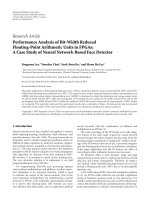
A concrete example may help to illustrate the
basic paradigm (Figure 1). Spivey et al. (2005)
asked participants to simply click with a
computer mouse the image of an object (e.g.,
“candle,” in Figure 1) that was identified
through headphones. The correct object was
paired either with a phonologically similar
distractor (e.g., “candy”), or with a dissimilar
control object (e.g., “jacket”). Their results
(Figure 1) show the curvature of the response
trajectories is affected by the similarity of the
paired object—the similar distractor produced
an increase in curvature, suggesting a
competitive “pull” during the response move-


4

Koop & Johnson (2012)

Figure 1. Example of response dynamics paradigm results
from Spivey et al. (2005). Increased response attraction
from a phonologically similar distractor produces greater
curvature in the response trajectory (gray line), relative to
a dissimilar control distractor (black line).

ment caused by an implicit desire to select the

phonologically similar distractor.
The current work presents the first (to our
knowledge) true extension of this body of
research to the domain within decision research
dealing with preferential choice. Previous
research using this paradigm has focused on
tasks such as identification and categorization
where objectively correct responses could be
determined a priori. In contrast, the remainder
of the current work will seek to validate the
method to situations where preferences are
more subjective, and extend it to a traditional
risky decision making task among gambles.
Anecdotal support (e.g., your finger’s
movements when selecting a cut of meat in the
grocer’s display case) and informal applications
(e.g., the online tracking of focus groups’
perceptions during presidential debates) to
preferential choice may abound. Here, however,
we hope to establish the scientific use of this
paradigm for decisions in a controlled
experimental design. We present two
experiments using this paradigm that establish
its validity and ability to address theoretical
predictions. We also provide enough detail for
researchers to consult as a sort of primer in
applying these methods and metrics in their
own research.
2. Experiment 1
Because this is the first extension of the

response dynamics method to preferential

choice, our first task is to demonstrate the
validity of the method within this domain. In
order to do so, we utilized an extremely wellstudied set of stimuli, the International
Affective Picture System (IAPS; Lang, Bradley,
& Cuthbert, 2008). The IAPS consists of over
1000 photographs that have been well normed
(by approximately 100 participants for each
picture) on three dimensions of emotion:
affective valence (or pleasantness), arousal, and
dominance. We focused on the dimensions of
pleasantness and arousal under the assumption
that preference would be roughly analogous to
ratings of pleasantness, given equal levels of
arousal. Thus we were able to directly test the
claim that measures of response dynamics can
accurately represent the development of
preference.
2.1. Methods
2.1.1. General paradigm
The general paradigm simply involves
participants making choices on a screen as
depicted in Figure 2. Participants began each
trial by clicking on a box at the bottom-center
of the screen. Once they did so, this box
disappeared and the picture stimuli (described
below) appeared in boxes at the upper-left and
upper-right of the screen. In this way, it was
possible to achieve a considerable distance

between the initiation and termination of the
response, as well as sufficient distance between

Figure 2. The general response dynamics paradigm.
Participants are initially presented with a “Start” button
and two empty response boxes, which are then populated
with response options once the “Start” button has been
clicked.


5

Koop & Johnson (2012)

the two response options. Clicking in the box of
their preferred picture recorded their choice,
removed the picture response boxes from the
display, and began the next trial. Immediate,
complete, and unadulterated preference for one
option would suggest that the response
trajectory proceeds in a straight line from the
point of initiation to the point of response.
Deviation from this direct path is interpreted as
an attraction to the competing (unchosen)
response option (e.g., Spivey & Dale, 2006). In
our case, this would suggest that even if a
participant selects Picture A, the degree of
curvature in the associated response trajectory
serves as an indication of implicit and
concurrent attraction towards Picture B during

the formation of the response—an online
measure of relative preference.
2.1.2. Participants
We recruited 98 employees at a corporate
business park to complete the experiment (59
female; age, M = 40.03 years, SD = 11.97; 13
left-handed). Between-subjects analyses did not
reveal any effects of handedness. Participants
signed-up for the experiment at a table in a
common area, where other experiment options
were also present. For their participation,
participants received product vouchers worth
approximately $10 for use at a company store.
2.1.3. Stimuli
All stimuli were drawn from the IAPS based
off of their previous ratings of average
pleasantness and arousal on nine-point scales
(Lang, et al, 2008). We selected 140 pictures
that ranged from very unpleasant (pleasantness
= 1.66) to very pleasant (pleasantness = 8.34),
and paired pictures based on their similarity in
pleasantness ratings to create 70 trials. Arousal
rating was held constant (difference < 0.45)
within trial pairs. These 70 trials were further
divided into 7 trial classes (10 pairs per class)
depending on similarity in pleasantness ratings
between the pictures, ranging from similar
(difference ≈ 0) to dissimilar (difference ≈ 6).
The experiment was conducted in a professional
setting, which resulted in 10 picture pairs being

removed at the behest of the employer due to
their graphic content. The removed trials were

more likely to have come from more dissimilar
classes because these classes required more
strongly negative pictures to achieve such large
differences in pleasantness. This left slightly
unequal numbers of trials in each trial class (see
Table 1). Thus, we were left with a total of 60
picture pairs that varied in pleasantness ratings
but were each roughly matched for arousal.
2.1.4. Procedure
After
providing
informed
consent,
participants were led to individual testing
booths and provided with instruction slides on
the nature of the task. Participants were told
that they were going to be shown two pictures,
and they simply had to click on the picture they
preferred.
To insure that the response
trajectories reflected the natural accumulation of
preference rather than demand characteristics,
participants were not told their mouse
movements would be recorded, and were given
no special instructions or motivations regarding
mouse movements. Prior to beginning the
main task, participants completed a practice trial

without stimuli to ensure familiarity with the
response process.
Next, each participant
completed five practice trials with increasingly
unpleasant stimuli. The purpose of these trials
was to acclimatize participants to the range of
pleasantness they would see in the task and
were not included in analyses. Following these
five
acclimatization
trials,
participants
completed the main block of 60 trials. The
main block was randomized for each participant
both for left/right picture presentation, as well
as for trial order. Immediately following the
experiment, participants were given their
payment vouchers and thanked for their
participation.
2.2. Results
2.2.1. Aggregate-level data analysis
Our goal for Experiment 1 is to explore
whether the response dynamics methodology
was valid for a typical preference task.
Therefore, we will focus on those analyses that
we feel are best suited to achieving this end, but
are by no means exhaustive. We refer the
reader to previous work for additional details
about the rationale and procedural steps for

6

Koop & Johnson (2012)

many of the analyses we perform (in particular,
Spivey et al., 2005; Dale et al., 2007; and Duran
et al., 2010).
The choice data show that participants were
globally more likely to choose the picture in
each pair that was rated as more pleasant (Table
1)1, and a repeated-measures ANOVA revealed
an effect of Similarity on individual choice
proportions, F(5, 485) = 184.67, p < .01. These
outcome data represent an initial validation of
our assumption that the pleasantness ratings in
IAPS are an appropriate normed analogue to
preference. Furthermore, the data suggest that
the presentation format and procedure did not
have an idiosyncratic effect on choice behavior,
and we can dive more deeply into the response
trajectories without concern.
Rather than merely interpreting discrete
choices, response dynamics allows us to observe
the process underlying these choices. Because
we recorded mouse position at a rate of 100 Hz,
each trial necessarily produces a different
number of measurements based on response
time. For ease of direct comparison, we timenormalized the complete trajectory for each trial
of each participant into a series of 101 ordered

(x,y) pairs. These were calculated by including
the initial and terminal x,y-coordinates, followed
by linear interpolation of the positional data
stream at 99 equally-spaced time intervals
(Spivey et al., 2005, established this precedent
for all subsequent work).
Next, we explored whether the degree of
curvature was indeed indicative of increased
“competition” from the foregone option. In the
context of the current task, it stands to reason
that selections among pairs of similar stimuli
should produce more competition, and less
direct response paths, whereas choices made
among dissimilar stimuli should contain more
unequivocally preferred options and thus more
direct paths. To assess this claim, we examined
those trials in which participants chose the more
positive option. In highly dissimilar trials
(difference > 3), most participants never selected

the more unpleasant option. This is
understandable given the nature of the stimuli,
but unfortunately causes a substantial loss of
power in within-subjects analyses. Most likely,
the majority of these selections could be
considered “error” trials. For example, choice
of the less pleasant option within the Difference
≈ 6 trial class may have entailed choosing a
picture entitled “Starving Child” over one
entitled “Wedding.” Thus, we choose to focus

only on those trials where participants selected
the more pleasant option, and can therefore
quantify the competitive pull of non-chosen,
less pleasant options. That is, we address the
question of whether, given choice of the more
pleasant option in a pair, increased pleasantness
of the foregone option is associated with
increased “pull” revealed by curvature in the
response trajectory.
The resulting aggregate trajectories suggest
an effect of Similarity via the predicted ordinal
relationships in curvature between trajectories
(Figure 3). Choices of the more pleasant option
were most direct in the Difference ≈ 6 trial
class, where the more pleasant option is most
easily identifiable. With each successive increase
in pleasantness similarity, curvature in the
response trajectory also increased. This trend
culminated in the Difference ≈ 1 trial class,
which appears to be subject to the most
competitive pull from the non-chosen, less
pleasant option. As predicted, this pattern
indeed suggests increasing preference for the
non-chosen option, and an increasingly
powerful competitive pull therefrom, as pictures
become more similarly pleasant.
2.2.2. Individual-level data analysis

Trials where difference = 0 were not included in these analyses
because there was no meaningful way to divide those trials on

the basis of response. That is, they were excluded because there
is no More Pleasant or Less Pleasant response when
pleasantness is held constant.
1

The plots shown in Figure 3 necessarily
aggregate across participants for clarity and
power, but it is important to consider metrics
calculated on the level of the individual


Figure 3. Response trajectories for selections of the more positive option by difference class. Plots are
time-normalized to 101 time steps, plotted as offset (in pixels) from trial initiation point. Placement of
response box is approximate. Solid lines (moving from dark to light) represent the Difference = 1,
Difference = 2, and Difference = 3 trial classes respectively. Dashed lines (again moving from dark
to light) represent the Difference = 4, Difference = 5, and Difference = 6 trial classes respectively.

participant as well. Response dynamics provides
a number of methods for quantifying such
differences visible in the aggregate trajectory
plots. One benefit of such metrics is that they
are done on each individual trajectory, and then
averaged across trials within each condition for
each participant, which is important given the
dangers inherent in working solely with
aggregate data (e.g., Estes, 1956; Estes &
Maddox, 2005). For example, we calculated
measures of absolute deviation (Euclidean
distance) from a hypothetical direct response
path at each of the 101 time-normalized bins

mentioned above. Maximum absolute deviation
(MAD) is simply the maximum value in this set,
whereas average absolute deviation (AAD) is the
mathematical average across the entire timenormalized trajectory.
MAD is better at

highlighting differences occurring in the “heart”
of each trial, whereas AAD is less susceptible to
spurious outliers but constrained by endpoints
held in common by each trial. We calculated
MAD and AAD for each trial, for each
participant, and then calculated each
participant’s average of these metrics across all
trials within each condition where the more
pleasant option was selected. As expected based
on the aggregate response trajectories shown in
Figure 3, the analysis of individual data show
the six trajectories differ in both MAD, F(5,470)
= 34.60, p < .001, and AAD, F(5,470) = 25.60,
p < .001. Furthermore, the linear contrast for
each metric was also significant (Figure 4 a,b; p
< .001), which confirms that the trend visible in
the aggregate trajectories was not merely an
artifact of averaging.


Figure 4. Absolute deviation from a direct path in pixels for Experiment 1. (a) Maximum absolute deviation (MAD) and
(b) average absolute deviation (AAD) were computed for each trial class in Experiment 1. Similarity in pleasantness was
highest in the Difference = 1 trial class and lowest in the Difference = 6 trial class.

2.3. Discussion: Experiment 1
The results of Experiment 1 represent an
important validation of the response dynamics
paradigm within the domain of preferential
choice. To provide this validation, we utilized
extremely well-normed stimuli drawn from the
International Affective Picture System (IAPS;
Lang, Bradley, & Cuthbert, 2008), and
instructed participants to simply select the
picture that they preferred in a pair. The
analyses performed above suggest that response
dynamics can be effectively utilized to more
fully elucidate the preferential choice process.
We contend that the curvature in participants’
response trajectories was the product of the
similarity in preference between the choice
options, as operationalized by normed
pleasantness ratings. The ordinal relationships
in similarity between the six trial classes were
manifested in the aggregate response
trajectories. Selections of the more pleasant
options on the most dissimilar trials (Difference
≈ 6) were subject to the least competitive pull,
and with each successive increase in similarity,
competitive pull (i.e., curvature) increased as
well. These data support the fundamental
response dynamics assumption previously
validated in other domains (e.g., Spivey,
Grosjean, & Knoblich, 2005): curvature

produced in the motor response is the product
of competition between response options.
The general paradigm has been wellestablished in cognitive science, but the key
validation provided uniquely by this study is the
use of response dynamics in the domain of
preferential choice, where responses are based
on subjective evaluation rather than objective
criteria. Given this validation, we can now
proceed to apply the method to a traditional
risky decision-making task of gamble
selection—almost certainly the most common
task in decision research over the past few
decades.
Because these stimuli are more
complex, it is possible that participants will do
all of their assessment “offline” before initiating
the response movement. However, if response
dynamics are again able to record the process of
preference development, they will offer a
substantial increase in resolution relative to the
simple outcome analyses (i.e., discrete choice)
that have typically been performed on this type
of stimuli.
3. Experiment 2
We imported the response dynamics
paradigm into a standard laboratory risky
decision-making task of gamble selection. In
short, we utilized the same method as
Experiment 1, but populated the response

9

Koop & Johnson (2012)

Figure 5. Presentation of gambles in Experiment 2.

boxes with economic gambles rather than
pictures (Figure 5). We conducted Experiment
2 to further the primary goal of establishing the
response dynamics paradigm in the field of
preferential choice. To this end, we will explore
several quantitative measures, in addition to
those utilized in Experiment 1, that have been
reported in the previous literature using this
paradigm. We will then evaluate how these new
metrics contribute to our understanding of risky
choice behavior above and beyond existing
techniques.
3.1. Method
3.1.1. Participants
We recruited 197 undergraduate students
enrolled in an introductory psychology course
to participate in one of two conditions: a Gain
condition (N = 110) and a Loss condition (N =
87). Students selected the experiment from an
online sign-up site that included a number of
experiment options. For their participation,
students received course credit and a monetary
reward based on their performance in the task

(as described in section 3.1.3).
3.1.2. Stimuli
Stimuli in the form of single (nonzero)
outcome gambles were created as follows. First,
we created one gamble for each success
probability of 0.90, 0.80, 0.70, and 0.60. We
assigned outcome values to these success
probabilities in an attempt to approximately
equate EV; we attached outcome values of $60,
$70, $80, and $90, respectively, to the success
probabilities (e.g., win $60 with probability 0.90,

else nothing). Next, we subtracted $10 from the
outcome values of these four gambles to create
four additional stimuli (e.g., win $50 with
probability 0.90), then subtracted $10 from each
of those to create our final four stimuli (e.g.,
win $40 with probability 0.90). Finally, we
created by hand every possible pairwise
comparison among these twelve stimuli where
one gamble had a higher success probability,
but the other had a higher outcome value. This
resulted in a total of 43 trials, to which we also
added three trials with a dominant option. We
then attached negative signs to all of the
outcomes in these 46 Gain condition pairs to
create a second set of 46 gambles for the Loss
condition. Note that some of these trials were
ultimately excluded from analyses (section 3.2);
complete pairings (shown for the Gain

condition) can be found in the Appendix.
3.1.3. Procedure
After
providing
informed
consent,
participants were informed that they would earn
money based on their responses during the
experiment. The nature of the experiment
required extra time to process the response data
and calculate final payments—thus, participants
also filled out payment vouchers that linked
them to their choice data so that they could be
paid at the end of the week in which they took
the experiment. This process was thoroughly
explained to participants by the experimenter
and repeated on instruction slides. After filling
out the payment voucher, participants read
through computerized instruction slides that
explained the nature of the task. Participants
were told that they would be playing a series of
gambles for real money and that every gamble
they selected would be simulated in order to
determine a final payment amount.
The two conditions varied in regards to the
exact method used to calculate a final payment
in order to avoid the clearly undesirable
potential to have students “owing” us money in
the Loss condition. In the Gain condition, we
calculated final payment by taking each

participant’s average earnings per trial and
dividing that value by ten. In the Loss
condition, participants were truthfully told that
they had received a $10 “endowment” for the


10

Koop & Johnson (2012)

task and that every gamble they played would
subtract from this amount. The same formula
used to determine payment in the Gains
condition was also used in the Loss condition,
only rather than simply taking the average of all
gamble outcomes divided by ten, this amount
was then subtracted from the initial
“endowment” of $10. Participants in both
conditions were provided with their respective
method and told that, on average, they could
expect to earn around $5. Finally, in order to
ensure that they understood the manner in
which they were expected to indicate a choice,
they were shown animated example trials and
completed an example trial prior to the main
task. As in Experiment 1, participants were not
informed that their mouse movements were
being recorded, and were given no special
instructions
about

mouse
movement
whatsoever. All participants used their right
hands to complete the task.
All participants completed all 46 trials in their
respective conditions. The order in which
gambles appeared was randomized once (for
both conditions), and then this single order was
reversed
for
counterbalancing
across
participants. The left/right presentation order
of gambles within a pair was also
counterbalanced
between
participants.
Following completion of all experimental trials,
participants were reminded of the date and
location of their payment collection window
before being dismissed.
3.2. Results
Experiment 2 represents an increase in the
complexity of stimuli relative to Experiment 1,
which allows us to ask more complex questions
about the psychological processes underlying
participants’ decisions.
This increased
complexity also allows us to showcase the
diversity of analytic techniques made possible

by continuous response tracking, including
derivative measures such as velocity and
acceleration. We will base our analyses on a
simple comparison of risk attitudes, which is a
pervasive construct in decision research using
gamble stimuli such as these. In particular, we
will compare trials where the “safer” option was
chosen to those trials where the “riskier” option

was chosen, where risk is operationalized by
gamble variance, per convention in the field. 2
For these comparisons, we excluded the three
trials with a dominant option to keep such
“obvious” choices from inflating any measures.
3.2.1. Aggregate-level data analysis
As in Experiment 1, the choice data (Table 2)
provide an initial assessment of whether either
the method or the stimuli are idiosyncratic in a
way that prevents further generalization. These
data show that participants preferred the Safe
gamble in the domain of Gains, by a margin of
three to one. In the Loss domain, participants
preferred the Risky option, although the relative
strength of this preference was not quite as
extreme. These results are in line with typical
risk attitudes across gains and losses (Tversky &
Kahneman, 1981), and again affirm that the
methodology did not adversely affect behavior,
and that the stimuli created for this task were
not abnormal.

Again as in Experiment 1, we first plotted
the time-normalized trajectories aggregated
across trials and participants (Figure 6) 3 .
Specfically, to produce Figure 6, we separated
an individual’s trials into Risky and Safe choices.
For each participant, we then averaged across
the corresponding trajectories within each
Response condition. At this point, each
participant is represented by a single Risky
trajectory and a single Safe trajectory, unless
they did not make a single choice of one type
across all trials. For example, a participant who
made all Safe choices would have a Safe
trajectory aggregated across 43 trials but would
Because most of our stimulus pairs did not differ greatly in
expected value, we assumed that gamble variance was an
appropriate measure, rather than requiring use of the coefficient
of variation (see Weber, Shafir, & Blais, 2004).
3 To prepare the data for subsequent analyses, we recoded the xcoordinates of the mouse movement trajectories as necessary to
remove the artifact of left-right presentation order
counterbalancing.
2


Figure 6. Response trajectories for Gain and Loss domains. Plots are time-normalized to 101 time
steps, plotted as offset (in pixels) from trial initiation point. Placement of response box is
approximate. Total y-distance of all trajectories is approximately 300 pixels. Dashed lines show
aggregated trajectories for choice of Risky option, and solid lines show aggregated trajectories for
choice of Safe option, separately for Loss trials (gray lines) and Gain trials (dark lines).

not have a Risky trajectory. Finally, the plots
shown in Figure 6 were generated by then
aggregating these individual x- and y-vectors
across all participants within the associated
Domain-Response combination to produce
each plotted trajectory, and negating the xcoordinates for all Risky choices. Because a few
participants in each Domain had fully consistent
revealed risk attitudes and never made one type
of choice (Risky or Safe), sample sizes varied
slightly across conditions (Table 2 for sample
sizes).
Closer inspection of Figure 6 reveals a
number of interesting phenomena. For the Gain
condition (dark lines), the response trajectories
are clearly more direct for the Safe choices
(solid lines) compared to the Risky choices
(dotted lines). In fact, the Safe choice
trajectories never tend towards the Risky
option, but the Risky choice trajectories suggest
participants briefly consider the Safe option
before changing course towards the Risky

option they ultimately choose. In the Loss
condition (light lines), the relative curvature
across Risky and Safe choice trajectories is
reversed—greater curvature is associated with
selection of the Safe option. Comparisons
across Gains and Losses makes clear that the
easiest and most definite choice, as inferred
from the directness of the response trajectory,

was selection of a Safe Gain, whereas the most
difficult and conflicted choice was selection of
the Risky Gain. Any choice in the Loss domain
produced conflict between these two relative
extremes, with selection of the Risky Loss
seeming slightly easier and less equivocal. This
interaction between Domain and Response is
especially noteworthy in that it parallels the
choice data in the current experiment as well as
an abundance of previous research (cf. prospect
theory’s risk-seeking for losses and risk-aversion
for gains; Kahneman & Tversky, 1979).
Another distinct advantage of collecting
continuous positional data is the ability to


Figure 7. Velocity of trajectories shown in Figure 6, calculated as average pixel distance per time step across a
moving window of seven time steps for Gains (a) and Losses (b). The first time step of the associated window is
shown on the x-axis. Dashed lines show aggregated trajectories for choice of Risky option, and solid lines show
aggregated trajectories for choice of Safe option. Bars along x-axis approximate periods of significant divergence (p
<.05).

calculate derivatives such as velocity (Figure 7)
and acceleration (not shown). To do so, we
determined the Euclidean distance traveled in
x,y-coordinates per time step (velocity) or the
change therein (acceleration). These measures
were calculated over a moving window of seven
time steps for velocity and fourteen time steps
for acceleration—these windows were arbitrarily

selected to smooth the trajectories for ease of
interpretation. The qualitative pattern suggested
by most of the trajectories is consistent with a
quick initial movement to start the trial,
followed by a relatively slow and consistent
movement during most of the trial, followed by
a terminal increase in both speed and
acceleration of movement towards the selected
option. Most prominent, perhaps, is the
difference between the Risky and Safe choices
in the Gain condition (Figure 7a), where the
former shows the most pronounced example of

the pattern just described, but the latter shows
relatively smooth and consistent progression
towards the Safe response across the trial. In
contrast, both the Risky and Safe trajectories in
the Loss domain (Figure 7b) show similar
trends, although the terminal velocity and
acceleration are greater for Safe choices. The
Risky Gain trajectory also shows an earlier
terminal increase in speed relative to all other
trajectories.
If theoretical considerations
warrant, additional derivatives (like acceleration
or jerk) can also be explored in more detail.
3.2.2. Individual-level data analysis
One challenge in working with such rich data
is that these data are most easily presented in
aggregate form—presenting the mouse paths

for each individual could be overwhelming and
largely unintelligible on trials with substantial
noise. Although the aggregated data nicely


Koop & Johnson (2012)

demonstrate prospect theory’s risk aversion in
gains and risk seeking in losses, it is possible
that this pattern only represents some virtual
average participant that doesn’t truly exist. For
example, if half of the participants proceeded
directly to select the risky choice while the other
half moved directly to the safe choice and
hesitated before moving to select the risky
choice, the aggregate path would lie somewhere
in the middle and not reflect any observed
behavior.
In order to refute this possibility, we moved
to individual-level analyses and calculated MAD
for each participant’s average safe and risky
response trajectories. We then calculated a
difference score by subtracting the deviation on
the average safe choice from the deviation on
the average risky choice, for each participant. A
bimodal distribution of difference scores would
suggest our results were just a product of
averaging across subjects, whereas a unimodal
distribution would show that the aggregate
paths were representative of most participants

(cf. Spivey et al., 2005).
Because our
participants were not required to select both
risky and safe responses, there were again a
small number in each condition that showed
fully consistent revealed risk attitudes and so did
not exhibit a given response (Gain N = 7, Loss
N = 5) and were excluded from this analysis.
Histograms of the difference scores from the
remaining participants (Figure 8) show that
most participants exhibited the same pattern

Figure 8. Histograms of difference scores. The difference
(Risky – Safe) in mean maximum deviation from a
straight path, in pixels, was calculated for each participant
for Loss (dashed lines) and Gain (solid lines) conditions.

13

Figure 9. Significance tests for differences between Risky
and Safe response trajectories. Each point represents the
p-value for a t-test between the Risky and Safe response
trajectories at one time step, for Loss trials (open points)
and Gain trials (filled points). Dashed line represents p =
0.05.

seen in the aggregate data. In the Gain
condition the modal response was positive,
showing greater MAD in risky trials than in safe
trials. In the Loss condition the modal response

was negative, which again matched the pattern
depicted in the aggregate data. Finally, the
mean and variance of the empirical distributions
were used to create reference normal
distributions; Kolmogorov-Smirnov tests of
normality showed that neither empirical
distribution showed a statistically significant
difference from the corresponding normal
distribution (Gains, p = .75; Losses, p = .44).
Having established that the patterns in Figure
6 are not artifacts of aggregation, the task shifts
to quantifying the differences seen in the
aggregate plots. One method is to perform
traditional significance tests comparing the
trajectories at each of the 101 time steps (Spivey
et al., 2005; Dale et al., 2007; and Duran et al.,
2010). For example, we compared the Risky
trajectory x-coordinates with the Safe trajectory
x-coordinates, in separate paired-samples tests
for each of the Gain and Loss conditions. The
two-tailed p-values from these tests are shown
in Figure 9, where it can be seen that the Risky
and Safe responses consistently diverged (p <
0.05) from the 29th to 96th time steps for the
Gain domain, and from the 36th to 93rd time
steps for the Loss domain. Whereas we would
expect the trajectories not to differ at the


Koop & Johnson (2012)

beginning or end due to common starting and
final coordinates (after reflecting the Risky
choice trajectories across x = 0), we see that the
majority of the movement during the “heart” of
each trial showed statistically significant
divergence. This same technique can be applied
to the velocity profiles shown in Figure 7.
These profiles similarly showed statistically
significant differences (p < .05) across large
spans of time bins; see Figure 7. It is important
to note that for both Domains, the final
windows during which Risky and Safe velocities
statistically differed included the velocity peaks
of each profile.
Many other metrics can be calculated using
the positional data to investigate specific claims;
we report several illustrative calculations in
Table 2 that support the claim of significant
differences between the trajectories. As in
Experiment 1, these calculations were made on
each individual trajectory, and then averaged
across trials within the appropriate DomainResponse condition for each participant. This is
helpful especially in situations where individual
trends might be lost in the aggregation
necessary to produce interpretable plots such as
those in Figure 6.

14
First, we calculated the total x,y-distance

traveled by each trajectory (XYdist in Table 2;
Dale et al., 2007; Duran et al., 2010). Globally,
participants travelled further when making
Risky responses, F (1,183) = 12.91, p < .01, and
when choosing amongst losses, F(1,183) =
20.67, p < .01. However, these effects were not
independent of one another. Confirming the
trend seen in the aggregate trajectories,
participants took a more circuitous route when
making Risky responses in the realm of Gains,
whereas the opposite was true in the realm of
Losses (Figure 10a), as supported by a test of
the interaction: F(1,183) = 84.63, p < .01. The
total distance provides a nice summary statistic,
but we can further “unpack” its meaning with
additional measures. For example, a
demonstrably large distance would be achieved
by a trajectory that repeatedly wavered back and
forth between the response options before
making a selection. This behavior can be
decomposed using three other measures: the
number of directional changes along the x-axis,
AAD, and the time at which MAD is achieved
(MADtime). We next examined each of these
measures in turn.

Figure 10. Measures afforded by response dynamics: (a) Total distance travelled; (b) Reversals of direction on the x-axis;
(c) average absolute deviation, AAD; and (d) time to maximum absolute deviation, MAD.

To compare the number of directional
changes along the x-axis (Xflips; Duran et al.,
2010), we calculated the sign (s) for each
comparison of successive x-coordinates, st = (xt
– xt-1), for all time steps t = [2, 101], and then
counted the number of changes in sign, sign(st)
≠ sign(st-1), for all t = [3, 101]. This represents
an intuitive measure of instability, or
instantaneous reversal of the response intention.
Analysis of variance in the Xflips metric revealed
main effects of Response, F(1,183) = 8.58, p <
.01, and Domain, F(1,183) = 23.74, p < .01. In
the realm of Gains, participants showed the
greatest tendency for Xflips on Risky choices, yet
showed the opposite pattern in the realm of
Losses (Table 2), creating a Domain x Response
interaction (Figure 10b), F(1,183) = 29.93, p <
.01.
We further analyzed individual-level data by
computing AAD for each individual response
trajectory, as in Experiment 1. Recall this
measure of average deviation from a direct path
indicates a tendency towards the option during
deliberation that was not ultimately chosen
(Freeman & Ambady, 2010). Like the previous
two measures, AAD shows an effect of
Domain, with participants generally showing
more indecision in the realm of Losses, F(1,183)
= 11.22, p < .01. Although there was also a
main effect of Response, F(1,183) = 30.55, p <

.01, this strongly interacted with the Domain
condition, F(1,183) = 104.03, p < .01. Planned
comparisons showed that Gain responses went
significantly further towards the Safe option
before selecting the Risky option than vice
versa, but for Losses the opposite was again
true (Figure 10c).
Finally, we recorded the latency from the
beginning of the trial at which MAD was
achieved. Later MADtime suggests a longer
period of indecision before initiating sustained
movement in the direction of the final choice.
As expected based on the previously mentioned
deviation data, MADtime occurs later in the realm
of Losses than in the realm of Gains, F(1,183) =
56.18, p < .01, and later for Risky responses
compared with Safe responses, F(1,183) = 4.65.
p < .05. As with the previous metrics, Domain
and Response conditions interacted with one
another (Figure 10d), F(1,183) = 29.88, p < .01.

3.3. Discussion: Experiment 2
Experiment 2 allowed us to more fully
exhibit the capabilities of response dynamics in
decision-making tasks by way of more complex,
cognitively demanding stimuli like those that
have been commonly employed for decades in
decision research. The collection of analyses
presented in Experiment 2 gives a pretty good
assessment of the response characteristics for

each trajectory type, as well as the meaningful
differences between conditions. For Gains, Safe
choices seem to be determined relatively early
and with moderate, consistent approach
tendency. Risky choices are the product of at
least one “online preference reversal,” indicated
by initial slow movement towards the Safe
option but then a sudden and quick movement
towards the Risky option. For Losses, both
Risky and Safe choices are characterized by a
substantial period of consistent indecisive
movement, primarily along x = 0, before a
relatively quick movement towards the chosen
option. Still, the Safe Loss option is chosen
more reluctantly than the Risky Loss, as
suggested by greater curvature and a brief
period of movement towards the Risky option.
Losses, relative to Gains, show a longer period
of indecisiveness (later MADtime), as well as a
higher degree of vacillation between options
(greater distance traveled and more directional
changes along x). It is instructive to point out
that some of the more specific trends (Table 2),
including individual reversals as measured by
Xflips, are obscured or lost in the aggregate plots
(Figure 6), which highlights the importance of
the detailed analyses.
The derivative profiles of response
trajectories in Experiment 2 also showed
dissociations by Response and Domain. Most

notable was the contrast between Safe Gains,
which showed a smooth velocity profile, and
Risky Gains, which showed an abrupt spike in
velocity as participants settled on the risky
option (Figure 7a). Beyond highlighting
processing differences, these derivative profiles
can also be used to assess predictions from
sufficiently precise theoretical accounts, such as
sequential sampling models (Busemeyer &
Townsend, 1993; Diederich, 1997) and the leaky
competing accumulator model (LCA; Usher &


16

Koop & Johnson (2012)

McClelland, 2001; Wojnowicz, Ferguson, Dale,
& Spivey, 2009). During trials where there is
high competition between options, the LCA has
previously predicted a compressed derivative
profile, leading to higher peak velocity
(Wojnowicz et al., 2009). For example, the
great difference in peak velocity for Risky and
Safe choices in the Gain condition (Figure 7a)
may reflect the relative ease with which people
selected the Safe option and the difficulty of
selecting the Risky option.
4. General discussion
Over the course of two studies, we have

sought to validate the use of response dynamics
for preferential decision tasks (Experiment 1),
and demonstrate the utility of the method in a
more complex and common risky decisionmaking task (Experiment 2). We find it
remarkable that response dynamics reveal such
strong differences between some conditions for
such high-order tasks as preferential choice in
general, and risky decision making specifically.
Compared to the previous applications of this
paradigm cited in the introduction, Experiment
2 is more complex and arguably requires
substantially more cognitive effort. Even still,
the clear differences in our trajectories are
generally more pronounced than in the previous
applications (e.g., Wojnowicz et al., 2009, Figure
1). Another key extension of the current work
over previous research in this paradigm is that,
in our case, there is not an objectively correct
response option. That is, in previous work,
there was always a correct category or desired
response, which made analyses more
straightforward and allowed for a greater degree
of experimental control. In the current task,
studying subjective preference, there is no way
to assign participants to select specific options,
but rather their choices dictate to which
condition the resulting trajectory belongs.
Although this may present analytic challenges,
we believe the data presented above
demonstrate the utility of the method for

decision researchers looking for additional
methodological tools.
Although we feel as though these data
provide a compelling argument for the use of
continuous data collection to inform our

understanding of the decision process, a
common critique is that this method
unnecessarily adds a layer of complexity when
simpler traditional methods (e.g., RTs) would
suffice. When addressing this critique, it is
important to note that collecting continuous
response data in no way precludes the collection
and analysis of RT data. In fact, traditional
metrics like choice data and RT come “free”
with the method. However, we contend that
continuous response data offer a view of the
decision process that is unavailable with these
traditional metrics.
Recent work has
demonstrated a quantitative dissociation with
RT in a probabilistic learning task (Koop &
Johnson, 2011), yet the qualitative pattern of
data from Experiment 2 may provide the most
convincing argument yet for the use of response
dynamics.
Specifically, online preference
reversals (most dramatically demonstrated for
Risky choices in the Gain condition) are
wonderful examples of the need to consider

response dynamics above and beyond outcome
measures like reaction times. RT measures may
allow researchers to infer decision difficulty, yet
RT cannot distinguish between a slow,
consistent accumulation of preference toward
the option that is ultimately chosen, and a
discrete shift in preference during the decision
process. Even process-tracing of information
acquisition cannot reveal online preference
formation, such as the stark reversal of
intention just discussed, or the analysis of
directional changes during the response
movement.
4.1. Theoretical implications and future directions
These results are interesting in their own
right, yet the most exciting and profound
implications concern model evaluation and
comparison, which was not explicitly the goal of
Experiments 1 and 2. As mentioned in the
introduction, the number of process models of
decision making is growing, and their
similarities with respect to current dependent
variables are often quite high. The analysis of
response dynamics affords the opportunity,
where appropriate, to make distinctions about
the deliberation and response process that
differentiates among theoretical claims. These


17

Koop & Johnson (2012)

may employ some of the specific metrics
introduced here, such as the shape of the
trajectory, derivative measures such as velocity
and acceleration, as well as specific measures
such as XYdist, Xflips, and AAD. For example,
some models espouse “one-reason decisionmaking” which suggests that a decision-maker
remains indifferent between choice options
until one piece of information (cue, attribute)
immediately, reliably, and wholly determines a
response intention (e.g., Gigerenzer &
Goldstein, 1999). Other models, such as
evidence accumulation approaches, allow for
the fluctuation of preference among options
before one is ultimately selected (e.g.,
Busemeyer & Townsend, 1993; Diederich,
1997; Roe, Busemeyer, & Townsend, 2001;
Stewart, Chater, & Brown, 2006; Usher &
McClelland, 2001). In line with these models,
the response trajectories of individual
participants are considerably less smooth and
show more online changes in preference (cf. the
Xflips measure in Table 2), perhaps an indicator
of variability around the “mean drift” in such
accumulator models. The competing claims
from these two model classes, as well as others,
could easily be tested using several of the
measures introduced above. Furthermore, some

models are precise enough to make predictions
about derivative measures such as velocity and
acceleration that can now be subject to
empirical tests (Wojnowicz et al., 2009).
One promising avenue for future
implementation of this methodology will
combine the benefits of process tracing of
information acquisition via eye tracking with the
online measurement of preference. This could
provide an exciting opportunity to observe in
real time the impact of individual pieces of
information on the accumulation of preference
for a choice option, as posited by contemporary
decision theories such as decision field theory
(DFT; Busemeyer & Townsend, 1993;
Diederich, 1997; Roe, Busemeyer, & Townsend,
2001). Whereas DFT may have difficulty in
explaining the large preference reversals seen in
Risky Gain and Safe Loss choices, other
variants of sampling models such as Diederich’s
(1997) multiattribute dynamic decision models
allow for the fixed ordering of attribute

sampling that could produce such trajectories
given differences in the (signed) evidence that
each attribute contributes and the order and
amount of time inspecting each attribute.
The implicit nature of this methodology is
also especially applicable for models that do not
make specific sequential process predictions,

such as neural network models that are not
described as stepwise heuristics (e.g., Usher &
McClelland, 2001; Simon, Krawczyk, Holyoak,
2004; Glöckner & Betsch, 2008). For example,
the “coherence shifts” proposed by parallel
constraint satisfaction models (e.g., Glöckner &
Betsch, 2008; cf. “dominance structuring” of
Montgomery & Svenson, 1989) assume that
initial uncertainty about which option is
preferred is reconciled later in the choice
process. This might suggest initial hesitance
and/or vacillation in the response trajectories
that becomes more direct, quicker, and uniform
later in the process. Another example pertains
to the recent popularity of “dual systems”
approaches to decision making, which are often
cast as an “intuitive” system that is responsible
for decision making unless it is overridden by a
more controlled “deliberative” system (e.g.,
Kahneman & Frederick, 2002). This hypothesis
might also be tested using response dynamics,
where one might expect a trajectory that
proceeds towards one option (using the intuitive
system) before the deliberative system takes
over, perhaps producing a single Xflip followed
by a high velocity trajectory towards the other
option (if it predicts the alternate response). The
details of such hypothesis tests are reserved for
future work; but the advances of the current
work make it possible to entertain such

questions scientifically.
4.2. Conclusion
We hope to have opened up the possibility
for a whole new, qualitatively different, set of
tools for researchers to assess process models
of decision making in particular, and cognition,
more generally. While we have introduced here
several specific illustrations, metrics, and
comparisons afforded by this new approach, we
encourage researchers to develop these methods
further. Not only can these methods enhance
existing models and theoretical approaches, but


Koop & Johnson (2012)

it may also facilitate a dramatic change in the
way we perceive of a decision task. For
example, Spivey and colleagues (Spivey et al.,
2005; Spivey & Dale, 2006) note the similarity
of the response dynamics such as ours to
representations of competing attractor basins in

18
dynamic systems theory (see Townsend &
Busemeyer, 1989, 1995, for application to
decision making). We look forward to both the
analytical and theoretical progress that is
achieved by building upon the innovations of
the current work.

Bechara, A., Damasio, A. R., Damasio, H., & Anderson, S. W. (1994). Insensitivity to future consequences
following damage to human prefrontal cortex. Cognition, 50, 7-15.
Bröder, A., & Schiffer, S. (2003). Bayesian strategy assessment in multi-attribute decision making. Journal of
Behavioral Decision Making, 16, 193-213.
Busemeyer, J.R., & Townsend, J.T. (1993). Decision Field-Theory – A dynamic cognitive approach to
decision-making in an uncertain environment. Psychological Review, 100, 432-459.
Cisek, P., & Kalaska, J. (2005). Neural correlates of reaching decisions in dorsal premotor cortex:
Specification of multiple direction choices and final selection of action. Neuron, 45, 801-814
Clark, A. (1999). An embodied cognitive science? Trends in Cognitive Sciences, 3(9), 345-351.
Dale, R., Kehoe, C. E. & Spivey, M. J. (2007). Graded motor responses in the time course of categorizing
atypical exemplars. Memory and Cognition, 35, 15-28.
Dale, R., Roche, J., Snyder, K., & McCall, R. (2008). Exploring action dynamics as an index of pairedassociate learning. PLoS ONE, 3(3): e1728. doi:10.1371/journal.pone.0001728
Diederich, A. (1997). Dynamic stochastic models for decision making under time constraints. Journal of
Mathematical Psychology, 41, 260-274.
Duran, N. D., Dale, R., & McNamara, D. S. (in press). The action dynamics of overcoming the truth.
Psychonomic Bulletin and Review.
Estes, W. K. (1956). The problem of inference from curves based on group data. Psychological Bulletin, 53,
134-140.
Estes, W. K., & Maddox, W. T. (2005). Risks of drawing inferences about cognitive processes from model
fits to individual versus average performance. Psychonomic Bulletin and Review, 12, 403-408.
Förster, J., & Strack, F. (1997) Motor actions in retrieval of valenced information: A motor congruence effect.
Perceptual and Motor Skills, 85, 1419-1427.
Franco-Watkins, A. M., & Johnson, J. G. (2011). Decision moving window: Using interactive eye tracking to examine
decision processes. Manuscript submitted for publication.
Freeman, J.B. & Ambady, N. (2009). Motions of the hand expose the partial and parallel activation of
stereotypes. Psychological Science, 20, 1183-1188.
Freeman, J. B. & Ambady, N. (2010). MouseTracker: Software for studying real-time mental processing using
a computer mouse-tracking method. Behavior Research Methods, 42, 226-241.
Freeman, J. B., Ambady, N., Midgley, K. J., & Holcomb, P. J. (in press). The real-time link between person

perception and action: Brain potential evidence for dynamic continuity. Social Neuroscience.
Friedman, R.S., & Förster, J. (2002). The influence of approach and avoidance motor actions on creative
cognition. Journal of Experimental Social Psychology, 38, 41-55.
Gallagher, S. (2005). How the Body Shapes the Mind. Oxford University Press.
Gigerenzer, G., Todd, P.M., & The ABC Research Group. (1999). Simple heuristics that make us smart. New
York: Oxford University Press.
Gigerenzer, G. & Goldstein, D. G. (1999). Betting on one good reason: The take the best heuristic. In
Gigerenzer, G., Todd, P. M. & the ABC Research Group (Eds.), Simple Heuristics That Make Us Smart.
New York: Oxford University Press.
Glimcher, P. (2009). Choice: Towards a standard back-pocket model. In P.W. Glimcher, C.F. Camerer, E.
Fehr, & R.A. Poldrack (Eds.), Neuroeconomics: Decision making and the brain (pp. 503-522). Burlington, MA:
Academic Press.
Glöckner, A. & Betsch, T. (2008). Modeling option and strategy choice with connectionist networks:
Towards an integrative model of automatic and deliberative decision making. Judgment and Decision Making
Journal, 3, 215-228.


Koop & Johnson (2012)

19

Johnson, E.J., Schulte-Mecklenbeck, M., & Willemsen, M.C. (2008). Process models deserve process data:
Comment on Brandstätter, Gigerenzer, and Hertwig (2006). Psychological Review, 115, 263-272.
Johnson, J. G. (2009). Embodied cognition of movement decisions: A computational modeling approach. In
M. Raab, J. G. Johnson, & H. Heekeren (Eds.), Mind and motion: The bidirectional link between thought and
action. Progress in Brain Research, 174, 137-150.
Johnson, J. G. & Koop, G. (in preparation). Evaluating critical assumptions of process-tracing in decision
making.
Kahneman, D., & Frederick, S. (2002). Representativeness revisited: Attribute substitution in intuitive
judgment. In T. Gilovich, D. Griffin & D. Kahneman (Eds.), Heuristics and Biases: The Psychology of Intuitive

Judgment. Cambridge University Press, New York.
Kahneman, D. & Tversky, A. (1979). Prospect theory – Analysis of decision under risk. Econometrica, 47,
263-291.
Koop, G. J. & Johnson, J. G. (in press). Response dynamics: A new window on the decision process.
Judgment and Decision Making.
Lang, P. J., Bradley, M. M., & Cuthbert, B. N. (2008). International affective picture system (IAPS): Affective ratings of
pictures and instruction manual. Technical Report A-8. University of Florida, Gainesville, FL.
McKinstry, C., Dale, R., & Spivey, M. J. (2008). Action dynamics reveal parallel competition in decision
making. Psychological Science, 19, 22–24.
Montgomery, H. & Svenson, O. (Eds.). (1989). Process and structure in human decision making. Oxford, England:
John Wiley & Sons.
Oullier, O., & Basso, F. (2010). Embodied economics: how bodily information shapes the social
coordination dynamics of decision making. Philosophical Transactions of the Royal Society B: Biological Sciences,
365, 219-301.
Payne, J.W. (1976). Task complexity and contingent processing in decision-making – Information search and
protocol analysis. Organizational Behavior and Human Performance, 16, 366-387.
Payne, J.W., Bettman, J.R., & Johnson, E.J. (1992). Behavioral decision research – A constructive processing
perspective. Annual Review of Psychology, 43, 87 – 131.
Payne, J.W., Bettman, J.R., & Johnson, E.J. (1993). The adaptive decision maker. Cambridge University Press.
Raab, M., & Green, N. (2005). Motion as input: A functional explanation of movement effects on cognitive
processes. Perceptual and Motor Skills, 100, 333-348.
Raab, M., Johnson, J.G., & Heekeren, H. (Eds.). (2009). Mind and motion: The bidirectional link between thought
and action. Elsevier.
Rieskamp, J., Busemeyer, J. R., Mellers, B. A. (2006). Extending the bounds of rationality: Evidence and
theories of preferential choice. Journal of economic literature. 44, 631-661.
Roe, R.M., Busemeyer, J.R., & Townsend, J.T. (2001). Multialternative decision field theory: A dynamic
connectionist model of decision making. Psychological Review, 108, 370-392.
Schall, J. D. (2004). On building a bridge between brain and behavior. Annual Review of Psychology, 55, 23-50.
Shimojo, S., Simion, C., Shimojo, E., & Scheier, C. (2008). Gaze bias both reflects and influences preference.
Nature Neuroscience, 6, 1317-1322.

Simon, D., Krawczyk, D.C., & Holyoak, K.J. (2004). Construction of preferences by constraint satisfaction.
Psychological Science, 15, 331-336.
Song, J. H., & Nakayama, K. (2009). Hidden cognitive states revealed in choice reaching tasks. Trends in
Cognitive Sciences, 13(8), 360–366.
Spivey, M. J. (2008). The continuity of mind. Oxford University Press.
Spivey, M. J., & Dale, R. (2006). Continuous dynamics in real-time cognition. Current Directions in Psychological
Science, 15(5), 207-211.
Spivey, M.J., Grosjean, M., & Knoblich, G. (2005). Continuous attraction toward phonological competitors.
Proceedings of the National Academy of Sciences of the United States of America, 102, 10393-10398.
Stewart, N., Chater, N., & Brown, G.D.A. (2006). Decision by sampling. Cognitive Psychology, 53, 1-26.
Strack, F., Martin, L. L., & Stepper, S. (1988) Inhibiting and facilitating conditions of the human smile: A
non-obtrusive test of the facial feedback hypothesis. Journal of Personality and Social Psychology, 53, 768-777.
Thomas, L.E., & Lleras, A. (2007). Moving eyes and moving thought: On the spatial compatibility between
eye movements and cognition. Psychonomic Bulletin & Review, 14, 663-668.


Koop & Johnson (2012)

20

Townsend, J. T. & Busemeyer, J. R. (1989) Approach-avoidance: Return to dynamic decision behavior. In
Chizuko Izawa (Ed.) Current Issues in Cognitive Processes: The Tulane Flowerree Symposium on Cognition. Hillsdale,
NJ: Erlbaum.
Townsend, J. T., & Busemeyer, J. R. (1995) Dynamic representation of decision making. In R. F. Port and T.
van Gelder (Eds.) Mind as Motion. MIT press.
Tversky, A., & Kahneman, D. (1981). The framing of decisions and psychology of choice. Science, 211, 453458.
Usher, M., and McClelland, J. L. (2001). On the time course of perceptual choice: The leaky competing
accumulator model. Psychological Review, 108, 550-592.
Wedel, M., & Pieters, R. (2008). Eye tracking for visual marketing. Boston, MA: Now Publishers, Inc.
Wedell, D.H., & Senter, S.M. (1997). Looking and weighting in judgment and choice. Organizational Behavior

and Human Decision Processes, 70, 41-64.
Wilson, M. (2002). Six views of embodied cognition. Psychological Bulletin and Review, 9(4), 625-636.
Wojnowicz, M.T., Ferguson, M.J., Dale, R., & Spivey, M.J. (2009). The self-organization of explicit attitudes.
Psychological Science, 20(11), 1428-1435.


21

Koop & Johnson (2012)

Appendix
Pair
1
2
3
4
5
6
7
8
9
10
11
12
13
14
15
16
17
18

19
20
21
22
23
24
25
26
27
28
29
30
31
32
33
34
35
36
37
38
39
40
41
42
43

$X
$90
$50
$60

$50
$40
$90
$50
$60
$40
$60
$70
$50
$50
$40
$80
$80
$50
$80
$90
$70
$60
$70
$80
$50
$60
$80
$60
$40
$70
$40
$70
$90
$70

$70
$50
$70
$70
$70
$60
$70
$60
$60
$40

Gamble A
Pr($X)
EV
60%
54
90%
45
90%
54
80%
40
90%
36
60%
54
90%
45
90%
54

90%
36
70%
42
80%
56
80%
40
90%
45
90%
36
70%
56
60%
48
90%
45
70%
56
60%
54
70%
49
90%
54
70%
49
60%
48

80%
40
80%
48
60%
48
90%
54
90%
36
70%
49
90%
36
60%
42
60%
54
80%
56
80%
56
90%
45
70%
49
80%
56
70%
49

80%
48
60%
42
70%
42
80%
48
90%
36

Var
1944
225
324
400
144
1944
225
324
144
756
784
400
225
144
1344
1536
225
1344

1944
1029
324
1029
1536
400
576
1536
324
144
1029
144
1176
1944
784
784
225
1029
784
1029
576
1176
756
576
144

$X
$40
$90
$90

$90
$80
$60
$80
$80
$80
$90
$90
$80
$80
$70
$60
$60
$70
$50
$70
$40
$70
$50
$60
$70
$80
$70
$70
$70
$50
$60
$60
$80
$80

$50
$60
$80
$60
$60
$40
$60
$50
$50
$50

Gamble B
Pr($X)
EV
90%
36
60%
54
60%
54
60%
54
60%
48
80%
48
60%
48
60%
48

70%
56
60%
54
60%
54
60%
48
70%
56
60%
42
90%
54
80%
48
60%
42
80%
40
70%
49
90%
36
60%
42
90%
45
70%
42

60%
42
70%
56
80%
56
70%
49
80%
56
80%
40
70%
42
80%
48
70%
56
70%
56
90%
45
70%
42
60%
48
90%
54
80%
48

90%
36
70%
42
80%
40
90%
45
80%
40

Var diff
Var
144
1944
1944
1944
1536
576
1536
1536
1344
1944
1944
1536
1344
1176
324
576
1176

400
1029
144
1176
225
756
1176
1344
784
1029
784
400
756
576
1344
1344
225
756
1536
324
576
144
756
400
225
400

1800
1719
1620

1544
1392
1368
1311
1212
1200
1188
1160
1136
1119
1032
1020
960
951
944
915
885
852
804
780
776
768
752
705
640
629
612
600
600
560

559
531
507
460
453
432
420
356
351
256

For each gamble, $X denotes the single nonzero outcome, and Pr($X) denotes the probability of
obtaining that outcome. EV = expected value, $X∙Pr($X); Var = variance, $X 2∙Pr($X) – EV2; Var
diff = variance difference, |Var(A) – Var(B)|. Pairs 1-21 were classified as “Dissimilar” trials based
on the difference in variance between the two gambles. Pairs 23-43 were likewise classified as
“Similar” trials.