A comparative study on two different methods for calculating gravity effect of an uneven layer: Application to computation of bouguer gravity anomaly in the east Vietnam sea and adjacent

VNU Journal of Science: Mathematics – Physics, Vol. 36, No. 3 (2020) 106-114

Original Article

A Comparative Study on Two Different Methods
for Calculating Gravity Effect of an Uneven Layer:
Application to Computation of Bouguer Gravity Anomaly
in the East Vietnam Sea and Adjacent Areas
Luan Thanh Pham
Faculty of Physics, VNU University of Science, 334 Nguyen Trai, Thanh Xuan, Hanoi, Vietnam
Received 26 April 2020
Revised 06 May 2020; Accepted 20 June 2020

Abstract: Calculation of gravity anomaly caused by an uneven layer is essential for quantitative
interpretation. By comparing calculated anomalies with observed anomalies, we may infer some
parameters of subsurface structures. There are many different methods for computing gravity
effect of an uneven layer. This paper presents a comparative study of two different forward
methods such as the space domain method and the frequency domain method. The performance of
each method was evaluated on two synthetic models. Finally, the more effective method was
applied to calculate Bouguer gravity anomaly in the East Vietnam Sea and adjacent areas using the
latest available dataset from the TOPEX mission.
Keywords: Forward method, space domain, frequency domain, Bouguer gravity anomaly, Vietnam.

1. Introduction
The purpose of gravity methods in natural resources exploration is to determine the geometric
parameters of the density structures, including depth, slope, lateral boundaries, etc [1-7]. Knowledge
of the parameters of the gravity sources can be important for optimizing drilling operations as well as
estimating mineral deposits [8-10]. The gravity anomalies can be calculated from known or assumed
information and then compared with measured gravity anomalies to determine some source
parameters. A range of different methods have been developed to calculate gravity anomalies caused
by density structures. The methods can generally be divided into two main groups, namely the space

________
Corresponding author.

Email address:
https//doi.org/ 10.25073/2588-1124/vnumap.4515

106


N.V. A et al. / VNU Journal of Science: Mathematics – Physics, Vol. 36, No. 3 (2020) 106-114

107

domain methods, and the frequency domain methods. Numerous methods have been developed to
calculate gravity anomaly of 2D structures in the space domain [11-16]. Some authors (e.g. [17-23])
derived gravity anomaly expressions of 3D structures in the space domain. Several other authors have
presented the different methods for calculating gravity effect of 3D structures in the frequency domain
and converted the anomalies into space domain by the inverse Fourier transformation for further
analysis [24-27]. The above forward methods are essential in interpreting gravity data, because they
provide the basic equations for automatically estimating subsurface structures.
In this paper, I aim to review the performance of the popular forward methods such as the space
domain method of Rao et al. (1990) and the frequency domain method of Parker (1973) [20, 24].
These methods were tested on a simple model and then on a complex model. Additionally, Bouguer
gravity anomaly in the East Vietnam Sea and adjacent areas were also calculated using the more
effective method.
2. Methods
In order to calculate the gravity anomaly caused by an uneven layer, Rao et al. (1990) developed a
space domain method that divided the uneven subsurface structure into many rectangular prisms. In a
Cartesian coordinate system, let T and W be the half thickness and half width of one such prismatic
source with Z1 and Z2 are the depths to the top and bottom, respectively. The gravity anomaly of a

prism source at any observation (x, y) of a rectangular mesh is given as [20]
𝑋𝑌 𝑋 𝑅 − 𝑌 𝑌 𝑅 − 𝑋 𝑋2 𝑌2 𝑍2
(1)
∆𝑔(𝑥, 𝑦) = 𝐺∆ (𝑧 𝑎𝑡𝑎𝑛
+ 𝑙𝑛
+ 𝑙𝑛
)| | |
𝑧𝑅 2 𝑅 + 𝑌 2 𝑅 + 𝑋 𝑋1 𝑌1 𝑍1
where
𝑋1 = 𝑥 + 𝑇, 𝑋2 = 𝑥 − 𝑇, 𝑌1 = 𝑦 + 𝑊, 𝑌2 = 𝑦 − 𝑊, 𝑅 = √𝑋 2 + 𝑌 2 + 𝑍 2 ,
G is the universal gravitational constant and ∆ is density contrast of the layer. The total gravity
anomaly ∆𝑔𝑡𝑜𝑡𝑎𝑙 (𝑥, 𝑦) is determined by adding the anomaly of all prismatic sources.
Another method was developed by Parker (1973) for rapid calculating gravity and magnetic
anomalies in the frequency domain. The method used a sum of the Fourier transforms of the powers of
the interface topography h to calculate gravity anomalies. Following Parker (1973), the total gravity
anomaly ∆𝑔𝑡𝑜𝑡𝑎𝑙 (𝑥, 𝑦) caused by an uneven layer is given by [24]
∞

∆𝑔𝑡𝑜𝑡𝑎𝑙 (𝑥, 𝑦) = 2𝜋𝐺∆𝑧0 + 𝐹

−1

[2𝜋𝐺∆𝑒

(−|𝑘|𝑧0 )

∑
𝑛=1

(−|𝑘|)𝑛−1

𝐹[ℎ(𝑥, 𝑦)𝑛 ]]
𝑛!

(2)

where 𝐹[ ] is the Fourier transform operator, 𝐹 −1 [ ] is the inverse Fourier transform operator, 𝑧0 is the
mean depth of the interface and 𝑘 = √𝑘𝑥2 + 𝑘𝑦2 with 𝑘𝑥 and 𝑘𝑦 are the wavenumbers in the x and y
directions, respectively.
3. Synthetic models
In this section, I designed two different theoretical models with density contrast of 200 kg/m3 to
test the efficiency of the methods.


108

L.T. Pham / VNU Journal of Science: Mathematics – Physics, Vol. 36, No. 3 (2020) 106-114

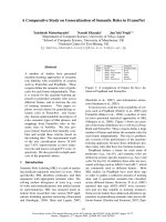
Figure 1. The 3D view of the first model.

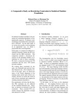
Figure 2. (a) The plan view of the first model, (b) The gravity anomalies calculated by the space domain method,
(c) The gravity anomalies calculated by the frequency domain method respectively, (d) The difference between
the results in Figure 2b and 2c.

Figure 1 displays the 3D view of the first model. Figure 2a displays the plan view of the model.
Figure 2b and 2c show the gravity anomalies calculated by the space domain method and the
frequency domain method respectively. It can be observed that the results obtained from applying the
methods are similar. The difference between these results is shown in Figure 2d. We can see that these
differences are insignificantly small and are in the range of -0.25 - +0.06 mgal. The root mean square

N.V. A et al. / VNU Journal of Science: Mathematics – Physics, Vol. 36, No. 3 (2020) 106-114

109

(RMS) error between them is only 0.0213 mgal. We note here that the frequency domain method took
only about 0.1838 s to compute the gravity anomalies at 64×64 grid nodes using a personal computer
with Intel (R) Core (TM) i3 at 2.40 GHz CPU, while the space domain method took about 22 s to
make the gravity model.

Figure 3. The 3D view of the second model.

Figure 4. (a) The plan view of the first model, (b) The gravity anomalies calculated by the space domain method,
(c) The gravity anomalies calculated by the frequency domain method respectively, (d) The difference between
the results in Figure 4b and 4c.

Since the very complex nature of the geological phenomena, it is necessary to also test the
efficiency of the methods in a more complex model. The 3D view of the complex model is shown in
Figure 3. Figure 4a displays the plan view of the model. The gravity anomalies calculated by the space
domain method and the frequency domain method are shown in Figure 4b and 4c, respectively. It can


110

L.T. Pham / VNU Journal of Science: Mathematics – Physics, Vol. 36, No. 3 (2020) 106-114

be seen from these figures that the result calculated by the space domain method compares reasonably
well with those obtained from using the frequency domain method. Figure 4d depicts the differences
of the gravity anomalies in Figure 4b and 4c. Clearly, these differences are very small, ranging from
+0.04 - +0.14 mgal. The RMS error between them is only 0.0661 mgal. In this case, the frequency
domain method took only about 0.2872 s to calculate the anomalies on a 2-D grid of 121×121 data,

while the space domain method took about 356 s on the same personal computer to make the similar
gravity model.
4. Application

Figure 5. Location of the East Vietnam Sea and adjacent areas.

Since the frequency domain method can perform fast computations with high precision, therefore
in this section, I applied it to calculate Bouguer gravity anomaly in the East Vietnam Sea and adjacent
areas. Location of the area is shown in Figure 5. The area lies between 100°E and 125°E of the
eastern longitudes and 0°N and 25°N of northern latitudes. To compile the Bouguer gravity map of
East Vietnam Sea and adjacent areas, we used the latest available data from the TOPEX mission,
which includes topographic data (version 18.1) and satellite-derived free-air gravity data (version
28.1) [28-30] ( The data have a grid cell size of 1 × 1 min.
Figure 6 and 7 show the topographic/bathymetric and free-air anomaly maps of the East Vietnam Sea
and adjacent areas. The terrain correction is computed using a crustal density of 2670 kg/m3 and seawater density of 1030 kg/m3, and shown in Figure 8. Figure 9 shows the complete Bouguer anomalies


N.V. A et al. / VNU Journal of Science: Mathematics – Physics, Vol. 36, No. 3 (2020) 106-114

111

after applying the terrain correction to the free-air anomalies. It can be seen from Figure 6 and 9 that in
general, the Bouguer anomalies are positive over ocean basins and negative over continental areas.
The inverse relationship between the Bouguer anomalies and topography is an isostasy manifestation.

Figure 6. The topographic/bathymetric map of the East Vietnam Sea and adjacent areas.

Figure 7. The Free-air anomaly map of the East Vietnam Sea and adjacent areas.

112

L.T. Pham / VNU Journal of Science: Mathematics – Physics, Vol. 36, No. 3 (2020) 106-114

Figure 8. The terrain correction for the East Vietnam Sea and adjacent areas.

Figure 9. The Bouguer gravity anomaly map for the East Vietnam Sea and adjacent areas.

5. Conclusion
I tried to review the performance of the use of the space domain method of Rao et al. (1990) and
the frequency domain method of Parker (1973) for calculating the gravity anomaly caused by an


N.V. A et al. / VNU Journal of Science: Mathematics – Physics, Vol. 36, No. 3 (2020) 106-114

113

uneven layer. Test studies were performed on two synthetic models. Although the results obtained
from application of the two methods are similar, the frequency domain method can perform very fast
computations for the gravity effects. Finally, I applied the frequency domain method for calculating
the Bouguer gravity anomaly in the East Vietnam Sea and adjacent areas using the latest available
dataset from the TOPEX mission. In this case, the forward of 1498×1498 observation point mesh took
only 195 s, which is a very short time for this type of calculation. Thus, it can be concluded that the
frequency domain method of Parker (1973) is an efficient tool for calculating the gravity anomaly of
the 3D structures, making an improved quantitative interpretation possible.
Acknowledgments
This research is funded by the Vietnam National University, Hanoi (VNU) under project number
QG.20.13.
References
[1] M.N. Nabighian, M.E. Ander, V.J.S. Grauch, R.O. Hansen, T.R. LaFehr, Y. Li, et al., Historical development of

the gravity method in exploration, Geophysics 70 (2005) 63–89.
[2] L.T. Pham, E. Oksum, T.D. Do, GCH_gravinv: A MATLAB-based program for inverting gravity anomalies over
sedimentary basins, Computers & Geosciences 120 (2018) 40–47.
[3] E. Oksum, M.N. Dolmaz, L.T. Pham, Inverting gravity anomalies over the Burdur sedimentary basin, SW
Turkey, Acta Geodaetica et Geophysica 54 (2019) 445–460.
[4] L.T. Pham, E. Oksum, T.D. Do, Edge enhancement of potential field data using the logistic function and the total
horizontal gradient, Acta Geodaetica et Geophysica 54 (2019) 143-155.
[5] L.T. Pham, T.D. Do, E. Oksum, S.T. Le, Estimation of Curie point depths in the Southern Vietnam continental
shelf using magnetic data, Vietnam Journal of Earth Sciences 41(2019) 216-228.
[6] A.M. Eldosouky, L.T. Pham, H. Mohammed, B. Pradhan, A comparative study of THG, AS, TA, Theta, TDX
and LTHG techniques for improving source boundaries detection of magnetic data using synthetic models: a case
study from G. Um Monqul, North Eastern Desert, Egypt, Journal of African Earth Sciences 170(2020) 103940.
[7] L.T. Pham, A comparative study on different filters for enhancing potential field source boundaries: synthetic
examples and a case study from the Song Hong Trough (Vietnam), Arabian Journal of Geosciences
13(2020) 723.
[8] L.T. Pham, T.V. Vu, S. Le-Thi, P.T. Trinh, Enhancement of Potential Field Source Boundaries Using an
Improved Logistic Filter, Pure and Applied Geophysics (2020). />[9] L.T. Pham, T.D. Do, Estimation of sedimentary basin depth using the hybrid technique for gravity data, VNU
Journal of Science: Mathematics – Physics, 33 (2017), 48-52.
[10] L.T. Pham, E. Oksum, T.D. Do, M.D. Vu, Comparison of different approaches of computing the tilt angle of the
total horizontal gradient and tilt angle of the analytic signal amplitude for detecting source edges, Bulletin of the
Mineral Research and Exploration 16(2020). />[11] M. Talwani, J. Worzel, M. Ladisman, Rapid gravity computations for two dimensional bodies with application to
the Mendocino submarine fracture zone, Journal of Geophysical Research 64 (1959) 49–59.
[12] I.V.R. Murthy, D.B. Rao, Gravity anomalies of two-dimensional bodies of irregular cross-section with density
contrast varying with depth, Geophysics 44 (1979) 1525–1530.
[13] I.V.R. Murthy, S.J. Rao, A Fortran 77 program for inverting gravity anomalies of two-dimensional basement
structures, Computers & Geosciences 15 (1989) 1149–1156
[14] J.J. Pan, Gravity anomalies of irregularly shaped two-dimensional bodies with constant horizontal density
gradient, Geophysics 54 (1989) 528–530.

114

L.T. Pham / VNU Journal of Science: Mathematics – Physics, Vol. 36, No. 3 (2020) 106-114

[15] V.C. Rao, V. Chakravarthi, M.L. Raju, Forward modeling: Gravity anomalies of two-dimensional bodies of
arbitrary shape with hyperbolic and parabolic density functions, Computers & Geosciences 20 (1994) 873-880.
[16] S.E. Oliva, C.L. Ravazzoli, Complex polynomials for the computation of 2D gravity anomalies, Geophysical
Prospecting 45 (1997) 809–818.
[17] M. Talwani, M. Ewing, Rapid computation of gravitational attraction of three-dimensional bodies of arbitrary
shape, Geophysics 25 (1960) 203-225.
[18] D. Nagy, The gravitational attraction of a right rectangular prism, Geophysics 31 (1966) 362–371.
[19] H.J. Goetze, B. Lahmerger, Application of threedimensional interactive modeling in gravity and magnetics,
Geophysics 53 (1988) 1096–1108.
[20] D.B. Rao, M.J. Prakash, N. Ramesh Babu, 3-D and 2 1/2-D modeling of gravity anomalies with variable density
contrast, Geophysical Prospecting 38 (1990) 411–422.
[21] H. Holstein, B. Ketteridge, Gravimetric analysis of uniform polyhedra, Geophysics 61 (1996) 357–364.
[22] B. Singh, D. Guptasarma, New method for fast computation of gravity and magnetic anomalies from arbitrary
polyhedra, Geophysics 66 (2001) 521–526.
[23] K. Mallesh, V. Chakravarthi, B. Ramamma, 3D gravity analysis in the spatial domain: model simulation by
multiple polygonal cross-sections coupled with exponential density contrast, Pure and Applied Geophysics 176
(2019) 2497–2511.
[24] R.L. Parker, The rapid calculation of potential anomalies, Geophysisical Journal of the Royal Astronomical
Society 31 (1973) 447–455.
[25] H. Granser, Three-dimensional interpretation of gravity data from sedimentary basins using an exponential
density-depth function, Geophysical Prospecting 35 (1987) 1030–1041.
[26] Y. Chai, W.J. Hinze, Gravity inversion of an interface above which the density contrast varies exponentially with
depth, Geophysics 53 (1988) 837–845.
[27] J. Feng, X. Meng, Z. Chen, S. Zhang, Three-dimensional density interface inversion of gravity anomalies in the
spectral domain, Journal of Geophysics and Engineering 11 (2014) 035001.
[28] W.H.F. Smith, D.T. Sandwell, Global seafloor topography from satellite altimetry and ship depth soundings,

Science 277 (1997) 1957-1962.
[29] D.T. Sandwell, E. Garcia, K. Soofi, P. Wessel, and W.H.F. Smith, Towards 1 mGal Global Marine Gravity from
CryoSat-2, Envisat, and Jason-1, The Leading Edge, 32 (2013) 892-899.
[30] D.T. Sandwell, R.D. Müller, W.H.F. Smith, E. Garcia, R. Francis, New global marine gravity model from
CryoSat-2 and Jason-1 reveals buried tectonic structure, Science 46 (2014) 65-67.