Observer-based sliding mode control for discrete nonlinear systems with packet losses: An eventtriggered method

Systems Science & Control Engineering
An Open Access Journal

ISSN: (Print) 2164-2583 (Online) Journal homepage: />
Observer-based sliding mode control for discrete
nonlinear systems with packet losses: an eventtriggered method
Xinyu Guan, Jun Hu, Yunfei Cui & Long Xu
To cite this article: Xinyu Guan, Jun Hu, Yunfei Cui & Long Xu (2020) Observer-based sliding
mode control for discrete nonlinear systems with packet losses: an event-triggered method,
Systems Science & Control Engineering, 8:1, 175-188, DOI: 10.1080/21642583.2020.1734986
To link to this article: />
© 2020 The Author(s). Published by Informa
UK Limited, trading as Taylor & Francis
Group.
Published online: 04 Mar 2020.

Submit your article to this journal

Article views: 266

View related articles

View Crossmark data

Full Terms & Conditions of access and use can be found at
/>

SYSTEMS SCIENCE & CONTROL ENGINEERING: AN OPEN ACCESS JOURNAL
2020, VOL. 8, NO. 1, 175–188
/>
Observer-based sliding mode control for discrete nonlinear systems with packet

losses: an event-triggered method
Xinyu Guana,b , Jun Hu

a,b,c , Yunfei Cuia,b

and Long Xua,b

a Department of Mathematics, Harbin University of Science and Technology, Harbin, People’s Republic of China; b Heilongjiang Provincial Key

Laboratory of Optimization Control and Intelligent Analysis for Complex Systems, Harbin University of Science and Technology, Harbin, People’s
Republic of China; c School of Engineering, University of South Wales, Pontypridd, UK
ABSTRACT

ARTICLE HISTORY

In this paper, the observer-based output feedback sliding mode control (SMC) problem is investigated for discrete delayed nonlinear systems subject to packet losses under the event-triggered
strategy. It is assumed that the packet losses may occur in the control channel from the sensor to
the observer. A suitable compensation strategy via the Bernoulli distributed random variable is used
to reduce the effects of packet losses. In order to avoid the phenomenon of network congestion during the networked transmission, an event-triggered mechanism is introduced to determine if the last
released measurement needs to be updated. Based on the zero-order-hold (ZOH) measurement, an
output feedback observer is designed to reconstruct the system state. This method can facilitate
the design of the discrete-time sliding surface. A sufficient condition is proposed to guarantee the
stochastic stability of sliding mode dynamics systems by using linear matrix inequality (LMI) method,
and a novel observer-based sliding mode controller is synthesized to force the trajectories of the
error systems onto the pre-designed sliding mode surface within finite time. Finally, an example is
given to illustrate the validity of the proposed theoretical result.

Received 2 January 2020
Accepted 23 February 2020

1. Introduction
The sliding mode control (SMC) is an effective control technique, which has been widely discussed in the
control theory (Kchaou & EI-Hajjaji, 2017; Zhang, Shi,
& Xia, 2010). The main idea of SMC is to select a suitable
sliding surface and design a discontinuous SMC law to
drive the system trajectories onto pre-designed sliding
surface, which can keep that the state trajectories stay in
the sliding surface thereafter (Cui, Hu, Wu, & Yang, 2019;
Zhang, Hu, Liu, & Zhang, 2018; Zhang, Hu, Zhang,
& Chen, 2020). The SMC has some great advantages compared with the conventional control methods such as the
insensitivity the matched parameter variations and external disturbances (Zhang et al., 2018). Therefore, the SMC
scheme has been widely used in the engineering fields,
such as robot manipulators, aircrafts, electrical motors
and so on (Tong, Lin, Huo, Jin, & Miao, 2020). Considerable
research efforts have been devoted to the SMC problems
for various systems, for example, fuzzy systems (Zhang
et al., 2010), uncertain systems (Zhang & Xia, 2010),
Markov jump systems (Chen, Guo, & Ma, 2019), stochastic systems (Liu, Wu, Wu, Luo, & Franquelo, 2019), and
discrete-time systems (That & Ha, 2015). Note that the

CONTACT Jun Hu

KEYWORDS

Event-triggered scheme;
sliding mode control; packet
losses; state observer; active
compensation

existence of the time delay would degrade the performance (Fei, Guan, & Gao, 2018; Fei, Shi, Wang, & Wu, 2018).

Recently, in Chen et al. (2019), the SMC problem has been
investigated for a class of uncertain discrete delayed systems with unmatched external disturbances and communication constraints.
In the practical applications, the data transmission is
periodic with sampling and transmission at a fixed time
interval in the networked environment (Hu, Wang, Liu,
Zhang, & Navaratne, 2020). Therefore, a huge sample
data needed to be calculated and transmitted. However, it is worth mentioning that the successive transmissions inevitably lead to unnecessary space occupancy
and energy waste. Therefore, there is a need to provide an effective method to determine whether the
sampled signals should be sent out or not, which is
commonly determined by certain criterion and guarantees the satisfactory performance (Dong, Wang, Shen,
& Ding, 2016; Hu, Liu, Zhang, & Liu, 2020; Zhang, Hu, Liu,
Yu, & Liu, 2019). Due to the above situation, much effort
has been devoted to present the proper communication
protocols (Chu & Li, 2019; Kumari, Bandyopadhyay, Kim,
& Shim, 2019). Recently, the event-triggered mechanism

,

© 2020 The Author(s). Published by Informa UK Limited, trading as Taylor & Francis Group.
This is an Open Access article distributed under the terms of the Creative Commons Attribution License ( which permits unrestricted use,
distribution, and reproduction in any medium, provided the original work is properly cited.


176

X. GUAN ET AL.

has been introduced and some related works with the
event-triggered scheme have been given (Lu, Hu, Guo,
& Zhou, 2018; Wu, Gao, Liu, & Li, 2017; Yao, Zhang, Li,

& Li, 2019). For example, based on the observer-based
control and state-feedback control scheme, the eventtriggered control problem of Markov jump systems (MJSs)
has been studied in Yao et al. (2019). In Song, Wang,
and Niu (2019), the token-dependent SMC law has been
proposed, which can force the trajectory of error systems onto the designed sliding mode surface and ensure
that the estimation error system is asymptotically stable. In Lu et al. (2018), the multi-delay stochastic NCS
has been discussed and the event-triggered scheme has
been proposed by using the free-weighting matrix (FWM)
method and the integral inequality method. Recently,
in Wu et al. (2017), the event-triggered SMC method
has successfully applied to multi-loop control by taking
the limitation of shared communication into account.
However, there are no results available on analysing
the observer-based SMC for discrete nonlinear systems
with the consideration of the event-triggered mechanism, which motivates us to cope with this challenging
and meaningful topic.
On another research front, the packet losses and
uncertain observations have been stirred much attention in the study of communication network (Dong, Hou,
Wang, & Ren, 2018; Dong, Wang, Ding, & Gao, 2016; Hu,
Wang, Liu, & Zhang, 2019; Tan & Liu, 2012, 2013; Tan,
Liu, & Duan, 2012; Tan, Liu, & Shi, 2015; Tan, Yin, Liu,
Huang, & Zhao, 2018). Generally, the packet losses are
modelled by the Bernoulli distribution and the Markov
chain (Hu, Zhang, Kao, Liu, & Chen, 2019; Hu, Zhang, Yu,
Liu, & Chen, 2019; Wang, Dong, Shen, & Gao, 2013). Consider the phenomenon of packet losses, which may occur
in a feedback loop of the communication network, the
discrete-time integral sliding mode surfaces have been
designed via the packet losses probability and the sliding mode controllers have been designed for network
control systems with continuous Markov packet losses
in Niu and Ho (2010) and Song, Chen, and Yam (2017),

respectively. In Xue, Yu, and Wang (2019), the H∞ control problem has been studied for discrete-time linear
time-delay systems with random packet losses and quantization. Besides, the sector-bounded method has been
applied to convert the quantitative control problem of
networked systems into a robust control problem with
uncertainty. Two different schemes for the uncertain linear systems involving packet losses have been considered, they are the hold-input method and zero-input
method (Yang, Wang, Niu, & Li, 2010), respectively. It is
devoted to the problem of robust output-feedback SMC
for the networked systems involving both measuring
and actuation consecutive data packet losses. In Argha,

Li, Su, and Nguyen (2016), a discrete-time SMC problem with robust output feedback and packet losses has
been studied. However, it should be noted that there is a
need to propose an event-based SMC scheme for discrete
networked systems with packet losses and time-varying
delays in order to fit the communication constraints.
Inspired by the above discussions, the main goal of this
paper is to solve the observer-based SMC problem for a
delayed system with event-triggered scheme and packet
losses. Here, the time-varying delays with known lower
and upper bounds are considered. Moreover, the packet
losses are addressed by utilizing a Bernoulli distributed
random variable. Then, an observer-based sliding mode
control method is given to fulfil the addressed problem.
The addressed problem has two challenges/difficulties
as follows: (1) How to deal with the effects of nonlinear disturbances, time-varying delays and parameteruncertainty on the discrete-time system simultaneously?
(2) How to propose an efficient control method to attenuate the effects from the phenomena of event-triggered
mechanism and packet losses onto the whole control performance? In summary, we adopt the following solutions.
Firstly, we handle the parameter uncertainties and nonlinear disturbances by using the norm-bounded conation
and Lipschitz method, which are addressed by utilizing
the linear matrix inequality technique. Moreover, to tackle

the effects of the event-triggered mechanism and packet
losses, the trigger condition and compensator are proposed, respectively. Based on the Lyapunov stability theory, the stochastic stability criterion is established for the
addressed discrete delayed system. Specifically, the main
contributions of this paper are listed as follows. (1) Both
the event-triggered mechanism and packet losses are,
for the first time, introduced together for the SMC problem in order to reflect a more realistic environment; (2) A
observer-based SMC method is given to compensate the
effects of time-delay, packet losses and event-triggered
mechanism; and (3) New sufficient condition is given to
ensure the stochastic stability of resulted sliding mode
dynamics and the reachability is shown.

2. Problem formulation and preliminaries
In this section, the brief problem formulation is given and
some useful lemmas are introduced.

2.1. System model
In this paper, the concerned discrete delayed nonlinear
system is described by
xk+1 = (A +
yk = Cxk ,

A)xk + Ad xk−τk + B(uk + f (xk )),


SYSTEMS SCIENCE & CONTROL ENGINEERING: AN OPEN ACCESS JOURNAL

xk = φk

∀ k ∈ [−τM , 0],

(1)

where xk ∈ Rn , uk ∈ Rm and yk ∈ Rp are the state vector, the control input and the output, respectively. A, Ad , B
and C are known constant matrices of appropriate dimensions. The parameter-uncertainty matrix A is assumed
to be norm-bounded of the following form:
A = EFH,

(2)

where F is an unknown matrix satisfying F T F ≤ I, E and
H are known constant matrices of appropriate dimensions. The nonlinear disturbance f (xk ) with known bound
satisfies
f (xk ) ≤ λ xk ,

Assumption 2.1: The positive integer τk describes the
discrete time-varying delay and satisfies
τm ≤ τk ≤ τM ,
with τm and τM being the bounds.

2.2. Packet losses
It is assumed that the packet losses will occur. In order to
compensate the packet losses, the following method will
be utilized in this paper:
yck =

yk ,

if data packet is received,

yk−1 , if data packet is lost.

¯
Pr{θk = 0} = 1 − θ,

k

exˆk ≥ δ xˆ kT¯ xˆ k¯ ,

(7)

where 0 < δ < 1 is a constant, and exˆk = xˆ k − xˆ k¯ with
xˆ k and xˆ k¯ being the current measurement and the last
released one, respectively.
> 0 is known weighting
matrix.
To end this section, the following lemmas are introduced to facilitate further derivations.
Lemma 2.1: For any real vectors a, b and matrix P > 0 of
appropriate dimensions, we have
aT b + bT a ≤ aT Pa + bT P−1 b.
Lemma 2.2: Let Q = QT , N and H be real matrices of appropriate dimensions. For any F satisfying F = F T ≤ I, Q +
NFH + HT F T NT < 0 if and only if there exists a scalar ε > 0
such that Q + εNNT + ε−1 HT H or equivalently
⎤
⎡
Q εN HT
⎣ ∗ −εI 0 ⎦ < 0.
∗
∗ −εI
Lemma 2.3 (Schur complement lemma): Given constant matrices S1 , S2 , S3 , where S1 = S1T and 0 < S2 = S2T ,

then S1 + S3T S2−1 S3 < 0 if and only if
S1
∗

S3T
<0
−S2

or

−S2
∗

S3
< 0.
S1

3. Observer-based sliding mode control

(5)

where 0 ≤ θ¯ < 1 stands for the probability. Equation (4)
can be rewritten in the following form:
yck = (1 − θk )yk + θk yk−1 .

eTxˆ

(4)

Equation (4) describes that yck is equal to yk when the

packet is perfectly received at time k, otherwise yck is
equal to yk−1 when a packet loss occurs. The probability of
packet losses is determined by the Bernoulli distribution
as follows:
¯
Pr{θk = 1} = θ,

the following event-triggered condition is introduced to
reduce the utilization of the network resources

(3)

where λ > 0 represents a known constant.

177

(6)

2.3. Event-triggered scheme
In this paper, the event detector is introduced to reduce
the network burdens and then save the limited communication resources. In particular, an event-triggered sampling strategy is used to determine whether or not the
current measurement output yk should be transmitted.
When the data is transmitted from observer to controller,

In this section, we aim to establish the event-triggered
SMC scheme for considered discrete-time networked system with packet losses. Firstly, an estimator is constructed
to estimate the unmeasurable state variables. In addition,
the observer-based controller is designed to force the
state trajectories onto the pre-designed sliding surface.
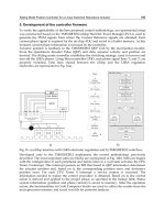
The detailed flowchart is given in Figure 1.

Remark 3.1: As illustrated in Figure 1, it is easy to see that
the signal transmitted is divided into the following steps.
Step 1: the original measurement output yk is obtained
at the time instant k. Step 2: the phenomenon of packet
losses is described when transmitting the signal, where a
random variable obeying the Bernoulli distribution is utilized. Therefore, the original measurement yk is replaced
by the updated signal yck . Step 3: a state observer is constructed in order to obtain the unmeasurable state variable. Step 4: the event-triggered is introduced to decrease
the network burdens, and the state variable xk¯ is transmit¯
ted to plant at the trigger instant k.


178

X. GUAN ET AL.

Figure 1. Event-triggered control with packet losses.

where G¯ = B(GB)−1 G. Hence, based on (1) and (8), the
error dynamic can be derived as

3.1. Estimator design
Firstly, the following state estimator is constructed:
¯ yk ],
xˆ k+1 = Aˆxk + Buk + L[yck − (1 − θ)ˆ
yˆ k = C xˆ k ,

ek+1 = [A +

+ Bf (xk ) − θk LCek−1 − θk LC xˆ k−1

(8)

where xˆ k ∈ Rn denotes the estimator state and L ∈ Rn×p
is estimator gain to be determined later.
The sliding mode surface is constructed as follows:
Sk = Gˆxk ,

(9)

where the matrix G ∈ Rm×n will be designed later to
ensure the non-singularity of GB.
According to SMC theory, when the system trajectories reach the sliding mode surface, the ideal condition
satisfies Sk+1 = Sk = 0. Therefore, we have
Sk+1 = Gˆxk+1
¯ yk )]
= G[Aˆxk + Buk + L(yck − (1 − θ)ˆ
= 0.

¯
+ [ A + (θk − θ)LC]ˆ
xk + Ad xˆ k−τk .

In this subsection, a sufficient condition is given to ensure
the stochastic stability of the sliding mode dynamics
based on the linear matrix inequality technique.
Theorem 3.1: Consider the sliding mode surface (9). Given
scalars ε1 > 0 and ε2 > 0, then the resulting closed-loop
systems composed of (13) and (14) are stochastically stable,
if there exist symmetric matrices P1 > 0, P2 > 0, Q2 > 0 and
W > 0 satisfying

⎡

The equivalent control law is then obtained as

¯
ukeq

−1

= −(GB)

¯ yk )].
G[Aˆxk¯ + L(yck − (1 − θ)ˆ

12

23 ⎦

22

∗

⎤

13

< 0,

BT P1 B < ε2 I,
where

11

=

11

12

∗

22

⎡ˆ

¯ xk + GAe
¯ xˆ
¯
− G)ˆ
xˆ k+1 = [A − (θk − θ)LC](I
k
¯
¯
+ (1 − θk )(I − G)LCe
k + θk (I − G)

11

(13)

11

⎢ ∗
=⎢
⎣ ∗
∗

,

−δ
δ −
∗
∗

(15)

−ε1 I

(12)

Substituting (12) into (8) yields

¯
xˆ k−1 ,
× LCek−1 + θk (I − G)LC

11

⎣ ∗
∗

(11)

By the event-triggered condition in (7), the eventtriggered equivalent control law can be rewritten as follows:

(14)

3.2. Stability analysis

(10)

¯ yk )].
ukeq = −(GB)−1 G[Aˆxk + L(yck − (1 − θ)ˆ

A − (1 − θk )LC]ek + Ad ek−τk

ˆ 13
0
ˆ 33
∗

ˆ 14 ⎤
0 ⎥
⎥
ˆ 34 ⎦ ,
−P2

(16)


SYSTEMS SCIENCE & CONTROL ENGINEERING: AN OPEN ACCESS JOURNAL

⎡

12

22

12

0
⎢ 0
=⎢
⎣ ˆ 35
0
⎡
−P2
⎢
=⎣ ∗
∗
=

¯ 12 =

1
¯ 12

1
¯ 13

1

¯ 21

1
¯ 22

13

1
23

ˆ 46
ˆ 66

ˆ 46

∗
0
¯ 12 ,

0
¯1

0
¯1

22

23

=

1
23
2
23

,

⎤

¯ 11 =

0 0 0 0 0 0 0 0 0 0
0
0 0 0 0 0 0 0 0 0 0 −ε1 I
√
√
¯ α2 = 2(1 − θ),
¯ α3 = 2 − θ,
¯
α1 = 5(1 − θ),
2
23

=

T

,

ˆ 11 = −P1 + (τM − τm + 2)P2 + 2AT P1 A

⎥
ATd P1 Ad ⎦ ,
ˆ 77

¯ 11
0

21

1
¯ 11

⎤
0
0 ⎥
⎥
ˆ 37 ⎦ ,
ˆ 46

0
0
ˆ 36
ˆ 46

179

¯ 2 λ2 I + δ
+ (6 + θ)ε

¯1
11
0

¯1
12
0

¯1
13 ,
0

,
√ T
⎤
3A P1 B
⎦,
0
0

⎡
0 3αC T W T
⎣
= 0
0
0
0
⎤
⎡√
¯ T P1 B

5αC T W T B θA
0
0
=⎣
0
0
AT P1 B
0 ⎦,
0
0
0
α3 AT P1
⎡
⎤
0
0
0
⎦
0
=⎣ 0
√ 0T T ,
T
T
T
T
α1 C W α2 C W B
3αC W
√
⎡√ ¯ T T
T

T
¯ T W T B⎤
6θC W C W
3θC
⎢
⎥
0
0
0
⎥,
=⎢
⎣
⎦
0
0
0
0
0
0
⎡√
3αC T W T
√ 0T T
⎢
¯ W
0
2
2θC
=⎢
⎣
0

0
0
0
⎤
√ 0T T
√ 0T T
¯ W B
2θC
3αC W ⎥
⎥,
⎦
0
0
0
0
⎤
⎡
0
0
⎥
⎢
0
0
⎥
⎢
⎥
⎢(1 − θ)C
T
T
¯ W E

0
⎥
⎢
⎢
¯ TWTE
¯ TWTE ⎥
= ⎢ −θC
−θC
⎥,
⎥
⎢
T
T
T
T
¯
¯
⎢ −θC W E
−θC W E ⎥
⎥
⎢
⎦
⎣
ATd P1 E
ATd P1 E
ATd P1 E
ATd P1 E
⎡√
⎤
3P1 E

0
⎢ 0
⎥
0
⎢
⎥
⎢ 0
⎥
0
⎢
⎥
⎢
⎥
=⎢ 0
0
⎥,
⎢
⎥
⎢ 0
⎥
0
⎢
⎥
⎣ 0
⎦
0
¯ 1E
0
(2 − θ)P

+ ε1 HT H,

ˆ 13 = (1 − θ)A
¯ T WC,
ˆ 14 = ˆ 15 = θA
¯ T WC,
¯ T WC,
ˆ 34 = ˆ 35 = −θA
ˆ 36 = ˆ 37 = AT P1 Ad − (1 − θ)C
¯ T W T Ad ,
ˆ 46 = −θ¯ C T W T Ad ,
ˆ 66 = 2AT P1 Ad − Q2 ,
d
ˆ 77 = 2AT P1 Ad − P2 ,
d
22

¯ T P1 B,
= −diag{P1 , P1 , BT P1 B, BT P1 B, θB
¯ 1 , (1 − θ)B
¯ T P1 B, P1 ,
BT P1 B, P1 , (1 − θ)P
¯ T P1 B, P1 , θP
¯ 1 , θB
¯ T P1 B, P1 },
θ¯ P1 , P1 , θB

ˆ 33 = (6 + θ)ε
¯ 2 λ2 I + (τM − τm + 1)Q2 − P1 + P2
+ ε1 HT H.

Here, G = BT P1 and L = P1−1 W is the observer gain.
Proof: Select the following Lyapunov–Krasovskii functional:
5
p

Vk =

Vk ,
p=1

Vk1 = xˆ kT P1 xˆ k ,
Vk2 = eTk P1 ek ,
−τm

r−1

xˆ iT P2 xˆ i ,
j=−τM +1 i=r+j

j=r−τk

−τm

g−1

Vk4

eTl Q2 el

=

l=g−τk

Vk5

=

r−1

xˆ jT P2 xˆ j +

Vk3 =

eTk−1 P2 ek−1

g−1

eTt Q2 et ,

+
l=−τM +1 t=l+g

T
+ xˆ k−1
P2 xˆ k−1 .

1 } − E{V 1 }, then we have
Defining E{ Vk1 } = E{Vk+1
k

¯ xk + GAe

¯ xˆ
¯
E{ Vk1 } = {[A − (θk − θ)LC](I
− G)ˆ
k
¯
+ (1 − θk )(I − G)LCe
k
¯
¯
+ θk (I − G)LCe
k−1 + θk (I − G)LC
¯ xk
¯
xˆ k−1 }T P1 {[A − (θk − θ)LC](I
− G)ˆ
¯ xˆ + (1 − θk )(I − G)LCe
¯
+ GAe
k
k


180

X. GUAN ET AL.

¯
¯
+ θk (I − G)LCe

k−1 + θk (I − G)LC

− 2α 2 xˆ kT C T LT P1 LC xˆ k−1

xˆ k−1 } − xˆ kT P1 xˆ k

+ 2α 2 xˆ kT C T LT GT (GB)−1 GLC xˆ k−1

¯ T P1 (I − G)Aˆ
¯ xk
= xˆ kT AT (I − G)

+ eTxˆ AT GT (GB)−1 GAexˆk
k

¯ T P1 GAe
¯ xˆ
+ 2ˆxkT AT (I − G)
k

¯ T C T LT P1 LCek
+ 2(1 − θ)e
k

¯ T P1 (I − G)LCe
¯
¯ x T AT (I − G)
+ 2(1 − θ)ˆ
k
k

¯ T C T LT GT (GB)−1 GLCek
+ 2(1 − θ)e
k

¯ T P1 (I − G)LCe
¯
+ 2θ¯ xˆ kT AT (I − G)
k−1

¯ T C T LT P1 LCek−1
+ 2θe
k−1

¯ T P1 (I − G)LC
¯
+ 2θ¯ xˆ kT AT (I − G)
xˆ k−1

¯ T C T LT GT (GB)−1 GLCek−1
+ 2θe
k−1

¯ T P1 (I − G)LC
¯
+ α 2 xˆ kT C T LT (I − G)
xˆ k

¯ T C T LT P1 LC xˆ k−1
+ 2θe

k−1

¯ T P1 (I − G)LCe
¯
+ 2α 2 xˆ kT C T LT (I − G)
k

¯ T C T LT GT (GB)−1 GLC xˆ k−1
− 2θe
k−1

¯ T P1 (I − G)LCe
¯
− 2α 2 xˆ kT C T LT (I − G)
k−1

T
+ 2θ¯ xˆ k−1
C T LT P1 LC xˆ k−1

¯ T P1 (I − G)LC
¯
− 2α 2 xˆ kT C T LT (I − G)
xˆ k−1

T
+ 2θ¯ xˆ k−1
C T LT GT (GB)−1 GLC xˆ k−1

¯ xˆ

+ eTxˆ AT G¯ T P1 GAe
k

− xˆ kT P1 xˆ k .

k

¯
¯ T AT G¯ T P1 (I − G)LCe
+ 2(1 − θ)e
k
xˆ
k

By applying Lemma 2.1, we can get

¯
¯ T AT G¯ T P1 (I − G)LCe
+ 2θe
k−1
xˆ
k

¯ x T AT GT (GB)−1 GLCek
− 2(1 − θ)ˆ
k

¯
¯ T AT G¯ T P1 (I − G)LC
+ 2θe

xˆ k−1
xˆ
k

¯ x T AT GT (GB)−1 GAˆxk
≤ (1 − θ)ˆ
k

¯ T P1 (I − G)LCe
¯
¯ T C T LT (I − G)
+ (1 − θ)e
k
k

¯ T C T LT P1 LCek ,
+ (1 − θ)e
k

¯ T P1 (I − G)LCe
¯
¯ T C T LT (I − G)
+ θe
k−1
k−1

≤ θ¯ xˆ kT AT GT (GB)−1 GAˆxk

T
¯ T P1 (I − G)LC

¯
+ θ¯ xˆ k−1
C T LT (I − G)
xˆ k−1

(17)

¯ 2 } = (1 − θ)
¯ θ¯ = α 2 ,
where G¯ = B(GB)−1 G, E{(θk − θ)
2
¯
¯ = 0. Next, it is
E{(θk − θ)(1
− θk )} = −α and E{θk − θ}
easy to obtain that
E{ Vk1 } ≤ 2ˆxkT AT P1 Aˆxk + 2ˆxkT AT GT (GB)−1 GAˆxk

¯ x T AT P1 LCek
+ 2(1 − θ)ˆ
k
¯ x T AT GT (GB)−1 GLCek
− 2(1 − θ)ˆ
k
+ 2θ¯ xˆ kT AT P1 LCek−1
− 2θ¯ xˆ kT AT GT (GB)−1 GLCek−1
+ 2θ¯ xˆ kT AT P1 LC xˆ k−1
− 2θ¯ xˆ kT AT GT (GB)−1 GLC xˆ k−1
+ 2α 2 xˆ kT C T LT P1 LC xˆ k
+ 2α 2 xˆ kT C T LT GT (GB)−1 GLC xˆ k

+ 2α 2 xˆ kT C T LT P1 LCek
− 2α 2 xˆ kT C T LT GT (GB)−1 GLCek
− 2α 2 xˆ kT C T LT P1 LCek−1
+ 2α 2 xˆ kT C T LT GT (GB)−1 GLCek−1

(19)

− 2θ¯ xˆ kT AT GT (GB)−1 GLCek−1

¯ T P1 (I − G)LC
¯
¯ T C T LT (I − G)
+ 2θe
xˆ k−1
k−1
− xˆ kT P1 xˆ k ,

(18)

¯ T C T LT P1 LCek−1 ,
+ θe
k−1

(20)

− 2θ¯ xˆ kT AT GT (GB)−1 GLC xˆ k−1
≤ θ¯ xˆ kT AT GT (GB)−1 GAˆxk
T
+ θ¯ xˆ k−1
C T LT P1 LC xˆ k−1 ,

(21)

− 2α 2 xˆ kT C T LT GT (GB)−1 GLCek
≤ α 2 xˆ kT C T LT GT (GB)−1 GLC xˆ k
+ α 2 eTk C T LT P1 LCek ,

(22)

2α 2 xˆ kT C T LT GT (GB)−1 GLCek−1
≤ α 2 xˆ kT C T LT GT (GB)−1 GLC xˆ k
+ α 2 eTk−1 C T LT P1 LCek−1 ,

(23)

2α 2 xˆ kT C T LT GT (GB)−1 GLC xˆ k−1
≤ α 2 xˆ kT C T LT GT (GB)−1 GLC xˆ k
T
+ α 2 xˆ k−1
C T LT P1 LC xˆ k−1 ,

(24)

¯ T C T LT GT (GB)−1 GLC xˆ k−1
− 2θe
k−1
≤ θ¯ eTk−1 C T LT GT (GB)−1 GLCek−1
T
+ θ¯ xˆ k−1
C T LT P1 LC xˆ k−1 ,

2α 2 xˆ kT C T LT P1 LCek

(25)


SYSTEMS SCIENCE & CONTROL ENGINEERING: AN OPEN ACCESS JOURNAL

≤ α 2 xˆ kT C T LT P1 LC xˆ k + α 2 eTk C T LT P1 LCek ,

− 2θ¯ eTk A¯ T P1 LC xˆ k−1 + 2eTk A¯ T P1 [ A

(26)

¯
xk + 2eTk A¯ T P1 Ad xˆ k−τk
+ (θk − θ)LC]ˆ

− 2α 2 xˆ kT C T LT P1 LCek−1
≤ α 2 xˆ kT C T LT P1 LC xˆ k

+ eTk−τk ATd P1 Ad ek−τk

+ α 2 eTk−1 C T LT P1 LCek−1 ,

+ 2eTk−τk ATd P1 Bf (xk )

(27)

− 2θ¯ eTk−τk ATd P1 LCek−1

− 2α 2 xˆ kT C T LT P1 LC xˆ k−1
≤ α 2 xˆ kT C T LT P1 LC xˆ k

− 2θ¯ eTk−τk ATd P1 LC xˆ k−1

T
+ α 2 xˆ k−1
C T LT P1 LC xˆ k−1 ,

(28)

+ 2eTk−τk ATd P1 Aˆxk

2θ¯ eTk−1 C T LT P1 LC xˆ k−1
≤

+ 2eTk−τk ATd P1 Ad xˆ k−τk

¯ T C T LT P1 LCek−1
θe
k−1

+ f T (xk )BT P1 Bf (xk )

T
+ θ¯ xˆ k−1
C T LT P1 LC xˆ k−1 .

(29)

¯ T (xk )BT P1 LCek−1
− 2θf

Substituting (19) and (29) into (18) and taking the mathematical expectation, one has

− 2θ¯ f T (xk )BT P1 LC xˆ k−1

E{

Vk1 }

≤

+ 2f T (xk )BT P1 Aˆxk

xˆ kT {2AT P1 A + 5α 2 C T LT P1 LC

+ 2f T (xk )BT P1 Ad xˆ k−τk

¯ T GT (GB)−1 GA + 5α 2 C T
+ (3 + θ)A

+ θ¯ eTk−1 C T LT P1 LCek−1

¯
GLC}ˆxk + eTk {3(1 − θ)

−1

T T

× L G (GB)

+ 2θ¯ eTk−1 C T LT P1 LC xˆ k−1

¯
× C L P1 LC + 2(1 − θ)
T T

T T T

−1

× C L G (GB)
T T

×C L

181

GLC + 2α

− 2θ¯ eTk−1 C T LT P1 Aˆxk

2

− 2θ¯ eTk−1 C T LT P1 Ad xˆ k−τk

¯ T LT P1 LC

P1 LC}ek + eTk−1 {4θC

− 2α 2 eTk−1 C T LT P1 LC xˆ k

¯ T LT GT (GB)−1 GLC
+ 3θC

T
+ θ¯ xˆ k−1
C T LT P1 LC xˆ k−1

T
¯ T LT
+ 2α C L P1 LC}ek−1 + xˆ k−1
{5θC
2 T T

¯ L G (GB)
× P1 LC + 2θC
T T T

−1

T
− 2θ¯ xˆ k−1
C T LT P1 Aˆxk

GLC

T

− 2θ¯ xˆ k−1
C T LT P1 Ad xˆ k−τk

2 T T

+ 2α C L P1 LC}ˆxk−1

T
− 2α 2 xˆ k−1
C T LT P1 LC xˆ k

¯ x T AT P1 LCek
+ 2(1 − θ)ˆ
k

+ xˆ kT AT P1 Aˆxk

+ 2θ¯ xˆ kT AT P1 LCek−1

+ 2ˆxkT AT P1 Ad xˆ k−τk

+ 2θ¯ xˆ kT AT P1 LC xˆ k−1

+ α 2 xˆ kT C T LT P1 LC xˆ k

+ eTxˆ AT GT (GB)−1 GAexˆk
k
− xˆ kT P1 xˆ k .
Besides,
¯ k + Ad ek−τ + Bf (xk ) − θk LCek−1

E{ Vk2 } = {Ae
k

T
+ xˆ k−τ
AT P1 Ad xˆ k−τk } − eTk P1 ek ,
k d

(30)

where A¯ = A +

A − (1 − θk )LC. Then, we obtain

E{ Vk2 } = eTk (A +

A)T P1 (A +

A)ek

¯
− θk LC xˆ k−1 + [ A + (θk − θ)LC]ˆ
xk

¯ T (A +
− 2(1 − θ)e
k

¯ k + Ad ek−τ
+ Ad xˆ k−τk }T P1 {Ae

k

¯ T C T LT P1 LCek
+ 2(1 − θ)e
k

+ Bf (xk ) − θk LCek−1 − θk LC xˆ k−1

+ 2eTk (A +

¯
+ [ A + (θk − θ)LC]ˆ
xk + Ad xˆ k−τk }

¯ T C T LT P1 Ad ek−τ
− 2(1 − θ)e
k
k

− eTk P1 ek

+ 2eTk (A +

¯ k + 2eT A¯ T P1 Ad ek−τ
= E{eTk A¯ T P1 Ae
k
k
¯ T A¯ T P1 LCek−1
+ 2eTk A¯ T P1 Bf (xk ) − 2θe
k

A)T P1 LCek

A)T P1 Ad ek−τk
A)T P1 Bf (xk )

¯ T C T LT P1 Bf (xk )
− 2(1 − θ)e
k
− 2θ¯ eTk (A +

A)T P1 LCek−1

(31)


182

X. GUAN ET AL.

¯ T (A +
− 2θe
k
+ 2eTk (A +

A)T P1 LC xˆ k−1

2eTk−τk ATd P1 Bf (xk )

A)T P1 Aˆxk

≤ eTk−τk ATd P1 Ad ek−τk

¯ T C T LT P1 Aˆxk
− 2(1 − θ)e
k

+ f T (xk )BT P1 Bf (xk ),

+ 2eTk (A +

¯ T (xk )BT P1 Bf (xk )
≤ θf

A)T P1 Aˆxk

¯ T C T LT P1 Aˆxk
− 2(1 − θ)e
k

¯ T C T LT P1 LCek−1 ,
+ θe
k−1

+ eTk−τk ATd P1 Ad ek−τk

− 2θ¯ f T (xk )BT P1 LC xˆ k−1

+ 2eTk−τk ATd P1 Bf (xk )

¯ T (xk )BT P1 Bf (xk )
≤ θf

¯ T AT P1 LC xˆ k−1
− 2θe
k−τk d

T

≤ f T (xk )BT P1 Bf (xk ) + xˆ kT AT P1 Aˆxk ,

(37)

2f T (xk )BT P1 Ad xˆ k−τk

+ 2eTk−τk ATd P1 Ad xˆ k−τk

≤ f T (xk )BT P1 Bf (xk )

+ f T (xk )BT P1 Bf (xk )

T
+ xˆ k−τ
AT P1 Ad xˆ k−τk ,
k d

¯ T (xk )BT P1 LCek−1
− 2θf

(38)

2θ¯ eTk−1 C T LT P1 LC xˆ k−1

¯ T (xk )BT P1 LC xˆ k−1
− 2θf

¯ T C T LT P1 LCek−1
≤ θe
k−1

+ 2f T (xk )BT P1 Aˆxk

T
+ θ¯ xˆ k−1
C T LT P1 LC xˆ k−1 ,

+ 2f T (xk )BT P1 Ad xˆ k−τk

2eTk (A +

¯ T C T LT P1 LCek−1
+ θe
k−1

(39)

A)T P1 Bf (xk )

≤ f T (xk )BT P1 Bf (xk )

¯ T C T LT P1 LC xˆ k−1
+ 2θe
k−1

+ eTk (A +

¯ T C T LT P1 Aˆxk
− 2θe
k−1

A)T P1 (A +

A)ek ,

(40)

¯ T C T LT P1 Bf (xk )
− 2(1 − θ)e
k

− 2α 2 eTk−1 C T LT P1 LC xˆ k

¯ T (xk )BT P1 Bf (xk )
≤ (1 − θ)f

¯ T C T LT P1 Ad xˆ k−τ
− 2θe
k−1
k

¯ T C T LT P1 LCek ,
+ (1 − θ)e
k

T
+ θ¯ xˆ k−1
C T LT P1 LC xˆ k−1

2eTk (A +

T
− 2θ¯ xˆ k−1
C T LT P1 Aˆxk

+ xˆ kT

T
− 2θ¯ xˆ k−1
C T LT P1 Ad xˆ k−τk

(41)

A)T P1 Aˆxk

≤ eTk (A +

T
− 2α 2 xˆ k−1
C T LT P1 LC xˆ k

A)T P1 (A +

A)ek

T

A P1 Aˆxk ,

(42)

− 2α 2 eTk−1 C T LT P1 LC xˆ k

+ xˆ kT AT P1 Aˆxk
+ 2ˆxkT AT P1 Ad xˆ k−τk

≤ α 2 eTk−1 C T LT P1 LCek−1

T
+ xˆ k−τ
AT P1 Ad xˆ k−τk
k d

+ α 2 xˆ kT C T LT P1 LC xˆ k ,

(43)

T
− 2α 2 xˆ k−1
C T LT P1 LC xˆ k

+ α 2 xˆ kT C T LT P1 LC xˆ k
(32)

≤ α 2 xˆ kT C T LT P1 LC xˆ k
T
+ α 2 xˆ k−1
C T LT P1 LC xˆ k−1 ,

By applying Lemma 2.1, it follows that

¯ T (A +
− 2(1 − θ)e
k

2α 2 eTk C T LT P1 LCLC xˆ k

¯ T (A +
≤ (1 − θ)e
k

α 2 eTk C T LT P1 LCek
+ α 2 xˆ kT C T LT P1 LC xˆ k ,

(36)

T

2f (xk )B P1 Aˆxk

+ 2eTk−τk ATd P1 Aˆxk

≤

(35)

T
C T LT P1 LC xˆ k−1 ,
+ θ¯ xˆ k−1

− 2θ¯ eTk−τk ATd P1 LCek−1

− eTk P1 ek .

(34)

¯ T (xk )BT P1 LCek−1
− 2θf

+ 2α 2 eTk C T LT P1 LC xˆ k

A)T P1 LCek
A)T P1 (A +

¯ T C T LT P1 LCek .
+ (1 − θ)e
k
(33)

(44)

A)ek
(45)


SYSTEMS SCIENCE & CONTROL ENGINEERING: AN OPEN ACCESS JOURNAL

According to (3), we have
E{ Vk3 } = E
2

≤ B P1 Bλ xk

r

r−1

xˆ jT P2 xˆ j −

⎩

j=r+1−τk+1

f T (xk )BT P1 Bf (xk )
T

⎧
⎨

2

≤

= ε2 λ2 IˆxkT xˆ k + ε2 λ2 IeTk ek .

j=−τM +1

(46)

r

⎝

+

xˆ jT P2 xˆ j
j=r−τk

⎛

−τm

ε2 λ2 IxkT xk

183

⎞

r−1

⎠ xˆ iT P2 xˆ i

−
i=r+j+1

i=r+j

⎫
⎬
⎭

≤ (τM − τm + 1)ˆxkT P2 xˆ k
Substituting (33)–(46) into (32), we obtain
¯ T (A +
E{ Vk2 } ≤ (4 − θ)e
k

A)T P1 (A +

T
− xˆ k−τ
P2 xˆ k−τk ,
k
⎧
g
⎨
4
E{ Vk } = E
eTl Q2 el −
⎩

A)ek

¯ T C T LT P1 LCek
+ 2(1 − θ)e
k
+ 2eTk (A +

−τm

+

¯ T C T LT P1 Ad ek−τ
− 2(1 − θ)e
k
k
A)T P1 LCek−1

¯ T (A +
− 2θe
k

A)T P1 LC xˆ k−1

l=−τM +1

eTl Q2 el

⎛

g

l=g−τk

g−1

⎝

⎠ eTt Q2 et

−
t=l+1+g

⎞

t=l+g

⎭

− eTk−τk Q2 ek−τk ,

(49)

E{ Vk5 } = eTk P2 ek − eTk−1 P2 ek−1 + xˆ kT P2 xˆ k

A)T P1 Ad xˆ k−τk

T
− xˆ k−1
P2 xˆ k−1 .

¯ T C T LT P1 Ad xˆ k−τ
− 2(1 − θ)e
k
k

(50)

In terms of the event-triggered condition (7), we can
achieve

+ α 2 eTk−1 C T LT P1 LCek−1
+ 2eTk−τk ATd P1 Ad ek−τk

δ xˆ kT xˆ k − 2δ xˆ kT exˆk + δeTxˆ

k

¯ T AT P1 LCek−1
− 2θe
k−τk d

exˆk − eTxˆ

k

exˆk ≥ 0.

(51)

Combining (30), (47) with (48)–(51), we have

¯ T AT P1 LC xˆ k−1
− 2θe
k−τk d

E{ Vk } ≤ ξ(k)T ϒ1 ξ(k),

+ 2eTk−τk ATd P1 Aˆxk

where

+ 2eTk−τk ATd P1 Ad xˆ k−τk

¯ T C T LT P1 Ad xˆ k−τ
− 2θe
k−1
k

T
ξ(k) = xˆ kT eTxˆ eTk eTk−1 xˆ k−1
k
⎡
ϒ11 −δ
ϒ13 ϒ14
⎢ ∗
ϒ
0
0
22
⎢

⎢ ∗
∗
ϒ
ϒ
⎢
33
34
⎢
ϒ1 = ⎢ ∗
∗
∗
ϒ44
⎢
⎢ ∗
∗
∗
∗
⎢
⎣ ∗
∗
∗
∗
∗
∗
∗
∗

T
+ 3θ¯ xˆ k−1
C T LT P1 LC xˆ k−1

ϒ11 = 3 AT P1 A + 9α 2 C T LT P1 LC − P1 + δ

¯ 2 λ2 Iˆx T xˆ k
+ (6 + θ)ε
k
¯ 2 λ2 IeT ek
+ (6 + θ)ε
k
+ (2θ¯ + 1)eTk−1 C T LT P1 LCek−1
¯ T C T LT P1 Aˆxk
− 2θe
k−1
+ α 2 eTk−1 C T LT P1 LCek−1

eTk−τk
ϒ15
0
ϒ35
0
ϒ55
∗
∗

T
xˆ k−τ
k

ϒ16
0

ϒ36
ϒ46
ϒ46
ϒ66
∗

T
− 2θ¯ xˆ k−1
C T LT P1 Aˆxk

+ (τM − τm + 2)P2 + 2AT P1 A

T
− 2θ¯ xˆ k−1
C T LT P1 Ad xˆ k−τk

¯ 2 λ2 I
+ 5α 2 C T LT GT (GB)−1 GLC + (6 + θ)ε

T
+ α 2 xˆ k−1
C T LT P1 LC xˆ k−1

¯ T GT (GB)−1 GA,
+ (3 + θ)A

+ 3ˆxkT AT P1 Aˆxk

¯ T P1 LC − (1 − θ)
¯ AT P1 LC,

ϒ13 = (1 − θ)A

+ 2ˆxkT AT P1 Ad xˆ k−τk

¯ T P1 LC − θ¯ AT P1 LC,
ϒ14 = ϒ15 = θA

T
+ 2ˆxk−τ
AT P1 Ad xˆ k−τk
k d

ϒ16 =

+ 4α 2 xˆ kT C T LT P1 LC xˆ k − eTk P1 ek ,

⎫
⎬

≤ (τM − τm + 1)eTk Q2 ek

¯ T C T LT P1 Aˆxk
− 2(1 − θ)e
k
+ 2eTk (A +

g−1

l=g+1−τk+1

A)T P1 Ad ek−τk

¯ T (A +
− 2θe
k

(48)

(47)

ϒ22 = δ

AT P1 Ad ,
−

+ AT GT (GB)−1 GA,

T

,
⎤

ϒ16
0 ⎥
⎥
ϒ36 ⎥
⎥
⎥
ϒ46 ⎥ ,
⎥

ϒ46 ⎥
⎥
ϒ67 ⎦
ϒ77


184

X. GUAN ET AL.

¯
ϒ33 = (4 − θ)(A
+

A)T P1 (A +

A) − P1 + P2

Proof: Take the following Lyapunov functional:

¯ 2 λ2 I + (τM − τm + 1)Q2
+ (6 + θ)ε

Vk6 = 12 STk Sk .

¯ T LT P1 LC
+ 3α 2 C T LT P1 LC + 5(1 − θ)C

The increment of Vk6 is deduced as follows:

¯ T LT GT (GB)−1 GLC,
+ 2(1 − θ)C
¯ +
ϒ34 = ϒ35 = −θ(A
ϒ36 = (A +

6
E{ Vk6 } = E{Vk+1
} − E{Vk6 }

A)T P1 LC,

= 12 STk+1 Sk+1 − 12 STk Sk

¯ T LT P1 Ad ,
A)T P1 Ad − (1 − θ)C

= 12 STk+1 Sk+1 − 12 STk Sk + STk Sk+1

¯ T LT P1 LC
ϒ44 = 3α 2 C T LT P1 LC + (1 + 6θ)C
¯ L G (GB)
+ 3θC
T T T

−1

− STk Sk+1

GLC − P2 ,

= STk Sk + 12 STk+1 STk − 12 STk STk

¯ L P1 Ad ,
ϒ46 = −θC
T T

= STk Sk +

¯ T LT P1 LC + 3α 2 C T LT P1 LC − P2
ϒ55 = 8θC

= STk Sk+1 − STk Sk +

¯ T LT GT (GB)−1 GLC,
+ 2θC

with

ϒ66 = 2ATd P1 Ad − Q2 ,

(54)

Sk = Sk+1 − Sk . Substituting (52) into (9), we have

¯ yk ) −
+ GL(yck − (1 − θ)ˆ

According to Lemmas 2.2–2.3 and letting W = P1 L, it
can be shown that the matrix inequality ϒ1 < 0 is ensured

by (15) and (16). Hence, if there exist matrices P1 > 0, P2 >
0, Q2 > 0, W > 0 and scalars ε1 > 0, ε2 > 0 satisfying (15)
and (16), then the sliding mode dynamic (13) and the error
dynamic (14) are stochastically stable.

= −GAexˆk −

sgn(Sk¯ ).

Theorem 4.1: Consider the state observer (8) and the sliding surface (9). For the real matrix G ∈ Rm×n and the gain
matrix L ∈ Rn×p , assume that the SMC law is synthesized as
¯ yk )
uk = −(GB)−1 [GAˆxk¯ + GL(yck − (1 − θ)ˆ
(52)

with

(55)

Therefore, considering the inequality Sk ≤ Sk
have
E{ Vk6 } = STk Sk +

+

In this section, the SMC law are designed to attenuate
the effects from an event-triggered mechanism and the
packet losses such that the system state can arrive at the
pre-specified sliding manifold within finite time.

sgn(Sk¯ )]}

¯ yk )
+ GL(yck − (1 − θ)ˆ

1
2

1
2

1,

we

STk Sk

= STk (−GAexˆk −

4. Observer-based sliding mode controller
design

> GA exˆk + ρ,
if STk sgn(Sk¯ ) > 0,
≤ −( GA exˆk + ρ), otherwise,

STk Sk ,

= GAˆxk + GB{−(GB)−1 [GAˆxk¯

ϒ77 = 2ATd P1 Ad − P2 .

sgn(Sk¯ )],

1
2

¯ yk )]
Sk+1 = G[Aˆxk + Buk + L(yck − (1 − θ)ˆ

ϒ67 = ATd P1 Ad ,

−

STk Sk

1
2

sgn(Sk¯ )) − STk Sk

STk Sk

≤ −ρ Sk − STk Sk +

1
2

STk Sk .

(56)

Based on the aforementioned discussion, it can be
known that Vk6 is negative through regulating the positive parameter ρ to be large enough for Sk = 0. Moreover,
Sk is reasonable bounded, which implies that the trajectory of system (1) can be maintained in the pre-defined
sliding motion. Consequently, the proof is complete.
Remark 4.1: The features of the main results can be summarized as follows: (1) there is a need to better characterize the packet losses and reflect the induced effects; and
(2) the event-triggered mechanism should be addressed
properly. Accordingly, the Equation (6) is introduced by
utilizing the random variable θk , where yck is employed
to construct the controller in (52). Moreover, the current
¯
instants are replaced by the trigger instants k.

(53)

where ρ is a positive constant, then the state trajectories can
be approached to the sliding manifold within finite time.

5. An illustrative example
In this section, an illustrative example is presented to
show the usefulness of the proposed theoretical results.


SYSTEMS SCIENCE & CONTROL ENGINEERING: AN OPEN ACCESS JOURNAL

185

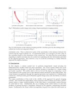
Figure 2. State and estimation.

Consider the system (1) with the following parameter
matrices:
A=

0.35
0.59
,
−0.04 −0.09

Ad =

−0.047 −0.68
,
0.002 −0.01

C=

2.5
,
1

H=

F = cos(0.3k),

B=
E=

0.25
,

0.8
0 0.01
0 0.01

T

,

0.1
0.25
,
0.01 −0.02

f (xk ) = cos(xk1 xk2 ).

The initial conditions of original system and state estimator are set as φk = [2 9]T , k ∈ [−5, 0] and xˆ 0 = [0 0]T ,
respectively. Consider the variation range of time delay as
τm = 2 and τM = 5. Select the corresponding probability
θ¯ = 0.45. Solving the LMIs (15) and (16) by utilizing Matlab LMI toolbox, the observer gain L and other parameters
matrices can be obtained as follows:
L=
P2 =

0.6641
1.8803

T

,

P1 =

4.7483 5.3530
,
5.3530 88.3364

47.5936 33.5355
,
33.5355 449.9477
δ = 0.41.

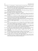
The simulation results are provided in Figures 2–4.
Figure 2 plots the state responses and estimation
responses. It is observed that the closed-loop system is
stochastically stable under the effect of packet losses and
event-triggered. In addition, the released intervals of the
observer to controller are shown in Figure 3. It can be seen

Figure 3. Released intervals from the observer to actuator channel.

that Figure 4 depicts the trajectories of the sliding mode
function Sk and the sliding mode controller uk . From the
simulation, it can be concluded that the proposed SMC
law generates desirable control signals to quickly drive
the state trajectories onto the sliding surface, which further illustrates the effectiveness of the developed SMC
scheme.

6. Conclusions
In this paper, the SMC problem has been investigated
for discrete delayed systems with event-triggered and

186

X. GUAN ET AL.

Figure 4. Control signal uk and trajectories of sliding variable Sk .

packet losses by designing the observer-based output
feedback controller. The discrete integral sliding surface
has been constructed. An SMC law has been synthesized such that the state trajectories of systems are driven
onto the neighbourhood of the specified sliding surface. Moreover, a sufficient condition has been given
to ensure the stochastic stability of the resulting sliding mode dynamics. Finally, a simulation example has
been given to demonstrate the effectiveness of the proposed control method. The further topic motivated by
the main results can be listed as: (1) the extension of
the method to observer-based SMC for networked systems with different communication transmission protocols as in Shen, Wang, Shen, Alsaadi, and Alsaadi (2020),
Liu, Wang, Chen, and Wei (2019), Wang, Wang, Chen,
and Sheng (2019), Zou, Wang, Hu, and Gao (2017), Zou,
Wang, Hu, and Zhou (2020) and quantized observation in Zou, Wang, Hu, and Han (2020), Liu, Wang, Han,
and Jiang (2020); (2) the discussion of the less conservatism of proposed SMC technique handling the delays.

Disclosure statement
No potential conflict of interest was reported by the author(s).

Funding
This work was supported in part by the National Natural
Science Foundation of China [grant number 61673141], the
European Regional Development Fund and Sêr Cymru Fellowship [grant number 80761-USW-059], the Outstanding Youth
Science Foundation of Heilongjiang Province of China [grant
number JC2018001], the Fundamental Research Foundation for

Universities of Heilongjiang Province of China and the Alexander von Humboldt Foundation of Germany.

ORCID
Jun Hu

/>
References
Argha, A., Li, L., Su, S., & Nguyen, H. (2016). Stabilising the networked control systems involving actuation and measurement consecutive packet losses. IET Control Theory and Applications, 10(11), 1269–1280.
Chen, S., Guo, J., & Ma, L. (2019). Sliding mode observer design
for discrete nonlinear time-delay systems with stochastic
communication protocol. International Journal of Control,
Automation and Systems, 17(7), 1666–1676.
Chu, X., & Li, M. (2019). H∞ non-fragile observer-based dynamic
event-triggered sliding mode control for nonlinear networked systems with sensor saturation and dead-zone input.
ISA Transactions, 94, 93–107.
Cui, Y., Hu, J., Wu, Z., & Yang, G. (2019). Finite-time sliding mode
control for networked singular Markovian jump systems with
packet losses: A delay-fractioning scheme. Neurocomputing.
doi:10.1016/j.neucom.2019.12.064
Dong, H., Hou, N., Wang, Z., & Ren, W. (2018). Varianceconstrained state estimation for complex networks with randomly varying topologies. IEEE Transactions on Neural Networks and Learning Systems, 29(7), 2757–2768.
Dong, H., Wang, Z., Ding, S. X., & Gao, H. (2016). On H∞ estimation of randomly occurring faults for a class of nonlinear
time-varying systems with fading channels. IEEE Transactions
on Automatic Control, 61(2), 479–484.
Dong, H., Wang, Z., Shen, B., & Ding, D. (2016). Varianceconstrained H∞ control for a class of nonlinear stochastic
discrete time-varying systems: The event-triggered design.
Automatica, 72, 28–36.
Fei, Z., Guan, C., & Gao, H. (2018). Exponential synchronization
of networked chaotic delayed neural network by a hybrid
event trigger scheme. IEEE Transactions on Neural Networks
and Learning Systems, 29(6), 2558–2567.

Fei, Z., Shi, S., Wang, Z., & Wu, L. (2018). Quasi-time-dependent
output control for discrete-time switched system with mode
dependent average dwell time. IEEE Transactions on Automatic Control, 63(8), 2647–2653.


SYSTEMS SCIENCE & CONTROL ENGINEERING: AN OPEN ACCESS JOURNAL

Hu, J., Liu, G.-P., Zhang, H., & Liu, H. (2020). On state estimation
for nonlinear dynamical networks with random sensor delays
and coupling strength under event-based communication
mechanism. Information Sciences, 511, 265–283.
Hu, J., Wang, Z., Liu, G.-P., & Zhang, H. (2019). Varianceconstrained recursive state estimation for time-varying complex networks with quantized measurements and uncertain inner coupling. IEEE Transactions on Neural Networks and
Learning Systems. doi:10.1109/TNNLS.2019.2927554
Hu, J., Wang, Z., Liu, G.-P., Zhang, H., & Navaratne, R. (2020). A
prediction-based approach to distributed filtering with missing measurements and communication delays through sensor networks. IEEE Transactions on Systems, Man and Cybernetics: Systems. doi:10.1109/TSMC.2020.2966977
Hu, J., Zhang, P., Kao, Y., Liu, H., & Chen, D. (2019). Sliding mode
control for Markovian jump repeated scalar nonlinear systems with packet dropouts: The uncertain occurrence probabilities case. Applied Mathematics and Computation, 362, Article number: 124574. Retrieved from />j.amc.2019.124574
Hu, J., Zhang, H., Yu, X., Liu, H., & Chen, D. (2019). Design
of sliding-mode-based control for nonlinear systems with
mixed-delays and packet losses under uncertain missing
probability. IEEE Transactions on Systems, Man and Cybernetics: Systems. doi:10.1109/TSMC.2019.2919513
Kchaou, M., & EI-Hajjaji, A. (2017). Resilient H∞ sliding mode
control for discrete-time descriptor fuzzy systems with multiple time delays. International Journal of Systems Science, 48(2),
288–301.
Kumari, K., Bandyopadhyay, B., Kim, K.-S., & Shim, H. (2019). Output feedback based event-triggered sliding mode control for
delta operator systems. Automatica, 103, 1–10.
Liu, S., Wang, Z., Chen, Y., & Wei, G. (2019). Protocol-based
unscented Kalman filtering in the presence of stochastic uncertainties. IEEE Transactions on Automatic Control.
doi:10.1109/TAC.2019.2929817
Liu, Q., Wang, Z., Han, Q.-L., & Jiang, C. (2020). Quadratic estimation for discrete time-varying non-Gaussian systems with

multiplicative noises and quantization effects. Automatica,
113, Art. no. 108714. Retrieved from />j.automatica.2019.108714
Liu, J., Wu, L., Wu, C., Luo, W., & Franquelo, L. G. (2019). Eventtriggering dissipative control of switched stochastic systems
via sliding mode. Automatic, 103, 261–273.
Lu, H., Hu, Y., Guo, C., & Zhou, W. (2018). State estimationbased event-triggered H∞ control for multi-delay stochastic
network control system. IEEE Access, 6, 74091–74103.
Niu, Y., & Ho, D. W. C. (2010). Design of sliding mode control subject to packet losses. IEEE Transactions on Automatic Control,
55(11), 2623–2628.
Shen, Y., Wang, Z., Shen, B., Alsaadi, F. E., & Alsaadi, F. E. (2020,
March). Fusion estimation for multi-rate linear repetitive processes under weighted try-once-discard protocol. Information Fusion, 55, 281–291.
Song, H., Chen, S.-C., & Yam, Y. (2017). Sliding mode control for
discrete-time systems with Markovian packet dropouts. IEEE
Transactions on Cybernetics, 47(11), 3669–3679.
Song, J., Wang, Z., & Niu, Y. (2019). On H∞ sliding mode control
under stochastic communication protocol. IEEE Transactions
on Automatic Control, 64(5), 2174–2181.
Tan, C., & Liu, G.-P. (2012). Consensus of networked multiagent systems via the networked predictive control and

187

relative outputs. Journal of the Franklin Institute, 349(7),
2343–2356.
Tan, C., & Liu, G.-P. (2013). Consensus of discrete-time linear networked multi-agent systems with communication
delays. IEEE Transactions on Automatic Control, 58(11), 2962–
2968.
Tan, C., Liu, G.-P., & Duan, G. (2012). Consensus of networked
multi-agent systems with communication delays based on
the networked predictive control scheme. International Journal of Control, 85(7), 851–867.
Tan, C., Liu, G.-P., & Shi, P. (2015). Consensus of networked
multi-agent systems with diverse time-varying communication delays. Journal of the Franklin Institute, 352(7),

2934–2950.
Tan, C., Yin, X., Liu, G.-P., Huang, J., & Zhao, Y. (2018). Predictionbased approach to output consensus of heterogeneous
multi-agent systems with delays. IET Control Theory and Applications, 12(1), 20–28.
That, N., & Ha, Q. (2015). Discrete-time sliding mode control with
state bounding for linear systems with time-varying delay
and unmatched disturbances. IET Control Theory and Applications, 9(11), 1700–1708.
Tong, M., Lin, W., Huo, X., Jin, Z., & Miao, C. (2020). A model-free
fuzzy adaptive trajectory tracking control algorithm based
on dynamic surface control. International Journal of Advanced
Robotic Systems, 17(1), Article number: 1729881419894417.
Retrieved from />Wang, Z., Dong, H., Shen, B., & Gao, H. (2013). Finite-horizon
H∞ filtering with missing measurements and quantization effects. IEEE Transactions on Automatic Control, 58(7),
1707–1718.
Wang, M., Wang, Z., Chen, Y., & Sheng, W. (2019). Event-based
adaptive neural tracking control for discrete-time stochastic nonlinear systems: A triggering threshold compensation
strategy. IEEE Transactions on Neural Networks and Learning
Systems. doi:10.1109/TNNLS.2019.2927595
Wu, L., Gao, Y., Liu, J., & Li, H. (2017). Event-triggered sliding
mode control of stochastic systems via output feedback.
Automatica, 82, 79–92.
Xue, B., Yu, H., & Wang, M. (2019). Robust H∞ output feedback control of networked control systems with discrete distributed delays subject to packet dropout and quantization.
IEEE Access, 7, 30313–30320.
Yang, F., Wang, W., Niu, Y., & Li, Y. (2010). Observer-based
H∞ control for networked systems with consecutive packet
delays and losses. International Journal of Control, Automation
and Systems, 8(4), 769–775.
Yao, D., Zhang, B., Li, P., & Li, H. (2019). Event-triggered sliding mode control of discrete-time Markov jump systems.
IEEE Transactions on Systems, Man, and Cybernetics: Systems,
49(10), 2016–2025.
Zhang, H., Hu, J., Liu, H., Yu, X., & Liu, F. (2019). Recursive state

estimation for time-varying complex networks subject to
missing measurements and stochastic inner coupling under
random access protocol. Neurocomputing, 346, 48–57.
Zhang, P., Hu, J., Liu, H., & Zhang, C. (2018). Sliding mode control
for networked systems with randomly varying nonlinearities
and stochastic communication delays under uncertain occurrence probabilities. Neurocomputing, 320, 1–11.
Zhang, P., Hu, J., Zhang, H., & Chen, D. (2020). H∞ sliding
mode control for Markovian jump systems with randomly
occurring uncertainties and repeated scalar nonlinearities


188

X. GUAN ET AL.

via delay-fractioning method. ISA Transactions. doi:10.1016/j.
isatra.2020.01.032
Zhang, J., Shi, P., & Xia, Y. (2010). Robust adaptive sliding-mode
control for fuzzy systems with mismatched uncertainties. IEEE
Transactions on Fuzzy Systems, 18(4), 700–711.
Zhang, J., & Xia, Y. (2010). Design of static output feedback
sliding mode control for uncertain linear systems. IEEE Transactions on Industrial Electronics, 57(6), 2161–2170.
Zou, L., Wang, Z., Hu, J., & Gao, H. (2017). On H∞ finite-horizon
filtering under stochastic protocol: Dealing with high-rate

communication networks. IEEE Transactions on Automatic
Control, 62(9), 4884–4890.
Zou, L., Wang, Z., Hu, J., & Han, Q.-L. (2020). Moving horizon estimation meets multi-sensor information fusion: Development,
opportunities and challenges. Information Fusion. doi:10.
1016/j.inffus.2020.01.009

Zou, L., Wang, Z., Hu, J., & Zhou, D.-H. (2020). Moving
horizon estimation with unknown inputs under dynamic
quantization effects. IEEE Transactions on Automatic Control.
doi:10.1109/TAC.2020.2968975