Approximation problems for dynamic equations on time scales , bài toán xấp xỉ cho phương trình động lực trên thang thời gian 624601

VIETNAM NATIONAL UNIVERSITY, HANOI
HANOI UNIVERSITY OF SCIENCE

Nguyen Thu Ha

APPROXIMATION PROBLEMS FOR DYNAMIC
EQUATIONS ON TIME SCALES

THESIS FOR THE DEGREE OF

DOCTOR OF PHILOSOPHY IN MATHEMATICS

HANOI

2017


VIETNAM NATIONAL UNIVERSITY, HANOI
HANOI UNIVERSITY OF SCIENCE

Nguyen Thu Ha

APPROXIMATION PROBLEMS FOR DYNAMIC
EQUATIONS ON TIME SCALES

Speciality: Differential and Integral Equations
Speciality Code: 62 46 01 03

THESIS FOR THE DEGREE OF

DOCTOR OF PHYLOSOPHY IN MATHEMATICS

Supervisor: PROF. DR. NGUYEN HUU DU

HANOI

2017


I HC QUăC GIA H
NáI
TRìNG I HC KHOA HC Tĩ NHI N

Nguyn Thu H

B I TO N X P X CHO PHìèNG TR NH

áNG

LĩC TR N THANG THI GIAN

Chuyản ng nh: Phữỡng trnh Vi phƠn v Tch phƠn
MÂ s: 62 46 01 03

LU N

NTI NS TO NHC

Ngữới hữợng dÔn khoa hồc:
GS. TS. NGUY N HU Dì

H NáI 2017


Contents

Abstract
Tâm t›t
List of Figures
List of Notations
Introduction
Chapter 1
1.1

Definition and example . . . . . . . . . .

1.2

Differentiation . . . . . . . . . . . . . . . . .
1.2.1.
1.2.2. Delta derivative . . . . . . . . . .

1.2.3. Nabla derivative . . . . . . . . . .
1.3

Delta and nabla integration . . . . . .
1.3.1.
1.3.2.
1.3.3.
1.3.4.

1.4

Exponential function . . . . . . . . . . . .
1.4.1.
1.4.2.
1.4.3.

1.5

Exponential stability of dynamic equ
i

1.5.1.


1.5.2. Exponential stability of linear

1.6 Hausdorff distance . . . . . . . . . . . . .
Chapter 2 On the convergence of solutions for dynamic equations
on time scales

2.1 Time scale theory in view of approxi

2.2 Convergence of solutions for -dynam
2.2.1.
2.2.2.
2.2.3.

2.3 On the convergence of solutions for n
scales . . . . . . . . . . . . . . . . . . . . . . .

2.3.1. Nabla exponential function . .
2.3.2.
2.3.3.
2.3.4.

2.4 Approximation of implicit dynamic eq
Chapter 3 On data-dependence of implicit dynamic equations on
time scales
3.1 Region of the uniformly exponential
3.1.1.
3.1.2.

3.2 Data-dependence of spectrum and e

dynamic equations . . . . . . . . . . . . .
3.2.1.

3.2.2. Solution of linear implicit dyna

3.2.3. Spectrum of linear implicit dy

ii

3.3 Data-dependence of stability radii . . . . . . . . . . . . . . . . . . . .


3.3.1. Stability radius of linear implicit dynamic equations . . . . . .
3.3.2. Data-dependence of stability radii . . . . . . . . . . . . . . . .
Conclusion

The author’s publications related to the thesis
Bibliography


Acknowledgments
First and foremost, I want to express my deep gratitude to Prof. Dr. Nguyen
Huu Du for accepting me as a PhD student and for his help and advice while I
was working on this thesis. He has always encouraged me in my work and
provided me with the freedom to elaborate my own ideas.
I also want to thank Dr. Do Duc Thuan and Dr. Le Cong Loi for all the help they
have given to me during my graduate study. I am so lucky to get their support.
I wish to thank the other professors and lecturers at Faculty of Mathematics, Mechanics and Informatics, Hanoi University of Science for their teaching, continuous
support, tremendous research and study environment they have created. I also
thank to my classmates for their friendship and suggestion. I will never forget their
care and kindness. Thank you for all the help and making the class like a family.

Last, but not least, I would like to express my deepest gratitude to my family.
Without their unconditional love and support, I would not be able to do what I
have accomplished.

Hanoi, December 27, 2017
PhD student

Nguyen Thu Ha.

iv


Abstract
The characterization of analysis on time scales is the unification and expansion of

results obtained on the discrete and continuous time analysis. In some last
decades, the study of analysis theory on time scales leads to much more general
results and has many applications in diverse fields. One of the most important
problems in analysis on time scales is to study the quality and quantity of dynamic
equations such as long term behaviour of solutions; controllability; methods for
solving numer-ical solutions... In this thesis we want to study the analysis theory on
time scales under a new approach. That is, the analysis on time scales is also an
approxima-tion problem. Precisely, we consider the distance between the solutions
of different dynamical systems or study the continuous data-dependence of some
characters of dynamic equations.
The thesis is divided into two parts. Firstly, we consider the approximation problem
to solutions of a dynamic equation on time scales. We prove that the sequence of
1

solutions xn(t) of dynamic equation x = f(t; x) on time scales fT ng n=1 converges to
the solution x(t) of this dynamic equation on the time scale T if the sequence of
these time scales tends to the time scale T in Hausdorff topology. Moreover, we
can compare the convergent rate of solutions with the Hausdorff distance between
Tn and T when the function f satisfies the Lipschitz condition in both variables.
Next, we study the continuous dependence of some characters for the linear
implicit dynamic equation on the coefficients as well on the variation of time scales.
For the first step, we establish relations between the stability regions
corresponding a sequence of time scales when this sequence of time scales
converges in Hausdorff topology; after, we give some conditions ensuring the
continuity of the spectrum of matrix pairs; finally, we study the convergence of the
stability radii for implicit dynamic equations with general structured perturbations
on the both sides under the variation of the coefficients and time scales.

v

Tõm tt
c trững ca giÊi tch trản thang thới gian l thng nhĐt v m rng cĂc nghiản
cứu  t ữổc i vợi giÊi tch trản thới gian liản tửc hoc thới gian rới rc. Trong cĂc
thp niản va qua, viằc nghiản cứu lỵ thuyt giÊi tch trản thang thới gian cho ta
nhiu kt quÊ tng quĂt v cõ nhiu ứng dửng v o cĂc lắnh vỹc khĂc nhau. Mt
trong nhng b i toĂn quan trồng ca giÊi tch trản thang thới gian l nghiản cứu t
nh chĐt nh tnh v nh lữổng ca phữỡng trnh ng lỹc. Trong lun Ăn n y,
chúng tổi mun nghiản cứu lỵ thuyt giÊi tch trản thang thới gian theo cĂch tip
cn mợi. õ l giÊi tch trản thang thới gian cặn l b i toĂn xĐp x. Cử th hỡn, chúng
tổi xt khoÊng cĂch gia cĂc nghiằm ca cĂc hằ ng lỹc khĂc nhau v s nghiản
cứu sỹ phử thuc liản tửc ca mt s c trững ca phữỡng trnh ng lỹc theo d
liằu ca phữỡng trnh.
Lun Ăn bao gỗm hai phn chnh. Trữợc ht, chúng tổi xt b i toĂn xĐp x nghiằm
ca phữỡng trnh ng lỹc trản thang thới gian v chứng minh ữổc dÂy cĂc nghiằm
1

xn(t) ca phữỡng trnh x = f(t; x) trản dÂy thang thới gian tữỡng ứng fT ng n=1 s hi
tử n nghiằm x(t) ca phữỡng trnh n y trản thang thới gian T nu nhữ dÂy thang thới
gian n y hi tử v thang thới gian T theo khoÊng cĂch Hausdorff. Hỡn na, chúng tổi
cụng Ănh giĂ ữổc tc hi tử ca cĂc nghiằm theo tc hi tử ca dÂy thang thới gian
khi h m f thọa mÂn iu kiằn Lipschitz theo cÊ hai bin.

Tip theo, ta nghiản cứu sỹ phử thuc theo tham s v theo sỹ bin thiản ca thang
thới gian ca mt s c trững ca phữỡng trnh ng lỹc 'n tuyn tnh. Bữợc u
tiản, ta thit lp mi liản hằ gia cĂc min n nh tữỡng ứng ca dÂy cĂc thang
thới gian khi dÂy thang thới gian n y hi tử theo tổ pổ Hausdorff. Cui cũng,
chúng ta nghiản cứu sỹ hi tử ca bĂn knh n nh ca phữỡng trnh ng lỹc 'n
tuyn tnh chu nhiu cĐu trúc cÊ hai v ca phữỡng trnh khi cÊ hằ s v
thang thới gian u bin thiản.

vi


Declaration
This work has been completed at Hanoi University of Science, Vietnam National
University under the supervision of Prof. Dr. Nguyen Huu Du. I declare hereby that
the results presented in it are new and have never been used in any other thesis.

Author:

Nguyen Thu Ha

vii


List of Figures
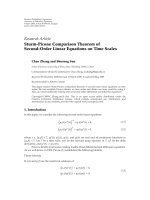
1.1 Points of the time scale T. . . . . . . . . . . . . . . . . . . . . . . . . 12
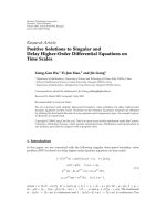
2.1 The graph of the solution xn(t) on the time scale Tn . . . . . . . . . . 49
2.2 The graph of the solution x4(t) on the time scale T4 . . . . . . . . . . 50
2.3 The graph of the solution xn(t) on the time scale Tn . . . . . . . . . . 55

viii


List of Notations
T
T
T

T
(t)
(t)
(t)
(t)
C(X; Y )
Crd(T; X)
1
Crd (T; X)
CrdR(T; X)
+

C ;C
d(x; X)
d(X; Y )
det A
e (t; s)
e (t; s)
b

)

f(t
GL(R )
=
<
K

Km

n

Im A
Ker A
rank A
L(X)
Ln

ix

m


N; Q; R; C

The set of natural, rational, real, complex numbers

N0

= N \ f0g
k

R(T ; X)

The set of regressive functions, defined on T

and take the value on X
R (T ; R)

+

k

The set of positive regressive function defined on T
and taking values in R

R+
UT = UT(T)

The set of positive real numbers
The uniformly exponential stability domain of time

scale T.
(A)

The set of the eigenvalues of the matrix A

(A; B)
S(T)

The set of solutions of det( A B) = 0
Exponential stability domain of time scale T

sup; inf

supremum, infimum

x

Introduction
The theory of ordinary differential equations (ODEs for short) is a theoretical sys-tem,
rather academic but going into the practical issues. In practical problems, ordinary
differential equations occur in many scientific disciplines, for instance in physics,
chemistry, biology, and economy. Under the name "modeling", the ordinary differential
equation is a useful tool to describe the evolution in times of population.
Therefore, studying the qualitative and quantitative properties of differential equa-tions
is important both in theory and practice. For the qualitative properties, the long term
behavior of the solutions has got many interests. The main tools in study-ing the
stability are Lyapunov functions, Lyapunov exponents or spectral analysis of matrices.
For the quantitative analysis, we have to find numerical approximations to the
solutions since almost ODEs can not be solved analytically. The Euler methods are
well-known because it is simple and useful, see [9, 19, 22, 63].
Besides, the theory of difference equations has a long term of history. Right from the
dawn of mathematics, it was used to describe the evolution of a lapin population with
the name "Fibonacci sequence". Difference equations might define the simplest
dynamical systems, but nevertheless, they play an important role in the investigation
of dynamical systems. The difference equations arise naturally when we want to study
mathematical models describing real life situations such as queuing problems,
stochastic time series, electrical networks, quanta in radiation, genetics in biology,
economy, psychology, sociology, etc., on a fixed period of time. They can also be
illustrated as discretization of continuous time systems in computing process.

On the other hand, in some last decades, the theory of time scales, under the
name Analysis on time scales, was introduced by Stefan Hilger in his PhD thesis
(supervised by Bernd Aulbach) in order to unify continuous and discrete analy-ses.
As soon as this theory was born, it has been received a lot of attention, see [6, 7,
13, 39, 41, 43]. Until now, there are thousands of books and articles dealt with the
theory of analysis on the time scale. Many familiar results concerning to
1

qualitative theory such as stability theory, oscillation, boundary value problem in
continuous and discrete times were "shifted" and "generalized" to the time scale.

Studying the theory of time scales leads also to some important applications
such as in the study of insect density model, nervous system, thermal
conversion process, the quantum mechanics and disease model.
One of the most important problems in the analysis on time scales is to investigate
dynamic equations. Many results concerning differential equations carry over quite
easily to corresponding results for the difference equations, while other results
seem to be completely different in nature from their continuous counterparts. The
study of dynamic equations on time scales gives a better perspective and reveals
such dis-crepancies between the differential equations and difference equations.
Moreover, it helps us avoid proving results twice, one for differential equations and
one for dif-ference equations. The general idea is to prove results for dynamic
equations where the domain definition of the unknown function is a so-called time
scale T, which is an arbitrary nonempty closed subset of real numbers R. By
choosing the time scale to be the set of real numbers R, the general result yields a
result concerning an ordinary differential equation as studies in a first course in
differential equations. On the other hand, if the time scale is the set of integers Z,
the same general result yields a result for difference equations.

However, studying the theory of dynamic equations on time scales leads to
much more general results since there are many more other complex time
scales than the above two sets. That is why so far the analysis on time scales is
still an attracted topic in mathematical analysis. Especially, there are still many
open problems in the studying dynamic equations on time scales.
The aim of this thesis is to consider the analysis on time scales under a new point of
view. That is not only a unification, but also in the view of approximation. Pre-cisely,

we want to consider the distance between the solutions of different dynamical systems
or to study the continuous dependence of some characters of dynamics equa-tions on
data such as spectrum, stability radii when both the coefficients and time scales vary.
The two following topics will be dealt with in this thesis:
1. Approximation of solutions

We begin firstly by analyzing the Euler method for solving the stiff initial value
problem. It is known that there are not many classes of ordinary differential equations for which we can represent explicitly their solutions via analysis formulas,
especially for nonlinear differential equations. Therefore, finding numerical solu2


tions of differential equations plays an important role in both theory and practice.
So far one proposes many algorithms to solve numerically solutions of a
differential equation. Among these algorithms, we have to take into account the
Euler explicit and implicit methods. Let us consider the initial value problem (IVP)
8
(0.1)
:x(t0) = x0:

The approximation of the solution x(t) of (0.1) will carry out at some different
values of times, say mesh points, on the interval [t0; T ]. To do that, for every n 2
N, we consider a partition of [t0; T ] consisting of points

t =t
0

(n)

0

Based on the points in (0.2), one constructs a difference equation
x0

(n)

( n)

= x0; xi +1 = xi

(n)

( n)

+ (ti +1

( n)

( n)

( n)

Then, the sequence of points (t k ; x k ), k = 1; :::; kn evaluates the points (t k ;
( n)

x(t k )), k = 1; 2; :::; kn on the solution curve starting from x0 at t0. We call this
approxima-tive way by Euler explicit method or Euler forward method.
Our problem is to give conditions of the function f and the partition (0.2)
ensuring the convergence of explicit Euler method:
sup x

k

j

(n)

k

These conditions can be found in [19, 22, 44].
Although the explicit Euler method is quite simple and easy to implement, even we
can carry out by portable calculators, and we can show the convergence of this
method. However, it has accumulation error in the processes of calculation and
Euler scheme can also be numerically unstable, especially for stiff equations since
explicit method requires impractically small time steps to keep the error in the
result bounded and the convergent rate is not good. Therefore, one deals with the
second Euler method, called Euler implicit method or Euler backward method. In
this method, instead of the equation (0.3), we consider the difference equation
( n)

(

n)

( n)

(

n)

( n)

x 0 = x0; x i+1 = x i + (t i+1
1; : : : ; kn 1:
(0.5)

(

n)

(

n)

t i )f(t i+1 ; x i+1 );

( n) ( n)
k ; x k ) in place of
( n)
approximation x i+1 appears on

This differs from the Euler explicit method in that the latter uses f(t
(

n)

(

i = 0;

n)

f(t i+1 ; x i+1 ). In Euler implicit method, the new
both sides of the equation (0.5) and thus the method needs to solve an algebraic
3


equation
x = y + hf(t; x);
where t; h and y are known and x is unknown. We can solve numerically the
solution x of (0.6) by iterative method
xk+1 = y + hf(t; xk); k = 0; 1; :::
By fixed point theorem, if h is sufficiently small and f satisfies Lipschitz condition
then xk ! x, which solves (0.6). It is clear that implicit methods require an extra
computation and they can be much harder to implement. However, people prefer
to use the Euler implicit method because many problems arising in practice are
stiff and it can achieve a higher convergent rate. The error at a specific time t is
O(h) (using the big O notation) and the Euler implicit method is in general
unconditionally stable. For a stiff problem, explicit methods need to take very
small time steps. Therefore, meanwhile the calculation is complicated, the Euler
implicit method could be preferred in this case (see [19, 22, 44]).
We now consider these two methods in different way. That is, when one
discretises the dynamic equation (0.1) on the real line [0; T ] by Euler explicit
method, we obtain the difference equation (0.3). On the time scale languages,
this equation is in fact the dynamic equation x (t) = f(t; x(t)) on time scale T n
r

described by (0.2). Similarly, the equation (0.5) is the dynamic equation x (t) = f(t;
x(t)) on Tn. When the mesh steps of Euler methods tend to 0, the sequence of
time scales Tn converges to T in some senses and the convergence of Euler
(n)

methods means the convergence of the sequence of solutions x ( ) , the solution
of above equations on the time scales Tn.
Therefore, for the first part of this thesis, we follow this idea to set up an approx1

imation problem in a more general context: Let T be a time scale and let fT ng n=1
be a sequence of time scales, which converges to T in some senses. Consider
the dynamic equation
8x (t)

:
where either t 2 T or t 2 T n. Assume that on every time scale Tn (resp. T), the
Cauchy problem of the equation (0.7) has a unique solution x n(t) (resp x(t)).
Then, the question here is whether we can specify conditions to have
xn( ) ! x( ) as n ! 1:
Further, how can we estimate the rate of this convergence?
4


We can also deal with a similar problem for the nabla dynamic equations on time
scales. That is instead of considering the equation (0.7), we study the equation

and put similar questions on
2. Continuous dependence of the spectrum and stability radius on data
The second topic dealt with in this thesis is to consider the data dependence of the
spectrum and stability radius for linear implicit dynamic equations on time scales.

In the recent years, several technical problems in electronic circuit theory and
robotic designs, chemical engineering, etc., see [15, 16, 28, 55] lead to the

problem of inves-tigating the dynamic implicit equation (IDEs for short)
f(X (t); X(t)) = 0;
where the leading term X can not be explicitly solved from X(t). The linear form
of this equation (LIDEs for short) is
AX (t) BX(t) = 0;
where A and B are two constant matrices (see [24, 46]). According to [24] and
[58], the investigation of the so-called index of the pencil of matrices fA; Bg is
necessary but the situation becomes more complicated. Note that if A is a
nonsingular matrix, then equation (0.11) can easily be reduced to an ordinary
1

differential equation by multiplying both sides of (0.11) by A . In this case, it is
known that if the original equation (0.11) is exponentially stable then it is still
stable under sufficiently small perturbations. In general case where A may be
degenerate, this property is no longer valid for the equation (0.11) since the
structure of the solutions of a LIDEs depends strongly on the index of fA; Bg
(see [31, 45, 46, 58]) and the solutions of (0.11) contain several components,
which are related by algebraic relations. Under perturbations, the index of the
system might be changed, which leads to the change of the algebraic relations.
In view of spectral theory, it is known that the uniformly exponential stability has
close relations with the spectrum (A; B) of the matrices pencil fA; Bg, i.e., the
set of roots of the equation det( A B) = 0: The changing in parameters of index
causes, without additional assumptions, the sharp change of the spectrum (A;
B) and the continuity of spectrum on the data is no longer valid.
5


Then, the question whenever the spectrum (A; B) depends continuously in fA;
Bg is important in both theory and practice. Thus, we come to the following
problem on time scales.

Problem: consider a family of linear implicit dynamic equations on the time
scales

T

n

Anx n (t) = Bnx(t); n 2 N;
mm

with An; Bn 2 C
. Which conditions ensure that the system Ax (t) = Bx(t) on the
time scale T is exponentially stable if the system (0.12) is exponentially stable
for every n and lim (An; Bn; Tn) = (A; B; T)?
n!1

In parallel, we have a similar problem for stability radii of implicit dynamic equations. It is well-known that if the trivial solution x 0 of the linear differential
0

system x = Bx (resp. difference system xn+1 = Bxn) is exponentially stable,
then for a small perturbation , the system
0

x = (B + D E)x
and respectively,
xn+1 = (B + D E)xn;
is still exponentially stable. Where is an unknown disturbance matrix and D; E are
known scaling matrices defining the structure" of the perturbation. The question rises
here: how large is possible in order to keep the stability of the system (0.13) (resp.
(0.14)). The threshold between the stability and instability, which measures the stability

robustness of system to such perturbation, is called the stability radius. It is defined as
the smallest (in norm) complex or real perturbations destabilizing the equation. If
complex perturbations are allowed, this measure is called the complex stability radius,
if only real perturbation are considered the real radius is obtained. The concept of
stability radii was introduced by Hinrichsen and Pritchard [48] in 1986 for linear timeinvariant systems of ordinary differential equations with respect to time-invariant input,
i.e., static perturbations. In this work, authors have shown that the complex stability
radius of linear differential equation (0.13) is given by

k

t2iR

max
Since then, this problems have been getting a lot of attentions from many research
groups of mathematics in the world. D. Hinrichsen and N.K Son [52] (1989) have
investigated the difference equation with the perturbation of the form x n+1 = (B + D
E)xn and have shown that the complex stability radius is computed by the
6


formula
!2C:j!j=1

max
To unify the equation (0.15) and (0.16), recently in [30], the authors give a
formula of the stability radius for the dynamic equation on time scales
x = Bx;
subjected to structure perturbations of the form
x = (B + D E)x:
The stability radius of (0.17) is given by

t2UTc

max
c

where UT is the uniform stability region of the time scale T and UT is the
comple-ment of UT.
The natural extension of the formula (0.18) to the implicit linear dynamic
equation on time scales belongs to [39]. In this work, authors consider the
stability radius of the linear implicit dynamic equation
Ax (t) = Bx(t);
subject to the perturbations
~~
[A;B]=[A;B]+D E =[A+D E1
where A; B 2 C
2C

m m

,D2C

m l

q m

; E1; E2 2 K

; E = [E1; E2], the perturbation

l q

. With these perturbations, the system (0.19) leads to

Axe (t) = Bxe(t);
authors have shown that the complex stability radius of the equation (0.19) is
given by the formula
r(A; B; D; E; T) =
where G( ) = ( E

1

2

E )( A

1

B) D:

We emphasise that the form (0.20) says that both sides of (0.19) are perturbed by .
As far as we know, the perturbation on the left side of (0.19) is very sensitive since
it can make its index change roughly. Following the analysis in [68], the stability
radius of the system (0.19) depends strongly in variation of the coefficients A; B.


7


Du-Lien-Linh for the first time in [36]; Du-Linh [32] and Du-Linh [34] consider
this continuous dependence under the statement of small parameters. They

claim that if r(E + "F; A; B; C) is the stability radius of
0

(E + "F )x = (A + B C)x;
Then, under some heavy assumptions, it is shown that
lim r(E + "F; A; B; C) = minfr(E; A; B; C); r(F22; A22; B2; C2)g;
"#0

where A =

In order to generalize this result, in this thesis we are concerned with the
following problem.
Problem: Let us consider a sequence of systems
Anx n (t) = Bnx(t);
mm

where An; Bn 2 C
; t 2 Tn and n 2 N. The leading coefficients A n; n 2 N; are
allowed to be singular matrices. We want to investigate the structure of stability
regions and their relation, give conditions ensuring the continuous dependence
on the data of the stability radii for implicit dynamic equations (0.23) when (A n;
Bn; Tn) converges.
The content of this thesis are as follows. Chapter 1 presents some basic knowledge
about time scales such as the definition of derivative, integration on time scales.
Besides, we give concepts of the exponential function, exponential stability region as
well as some results of the stability for the dynamic equations on time scales.

The second chapter is devoted to the study of the convergence of solutions to dynamic equations. We endow the set of time scales with the Hausdorff distance. Let
xn(t) (resp. x(t)) be the solution of the equation x = f(t; x) (or the nabla dynamic
r

equation x = f(t; x)) on time scale T n (resp. on T). Under the assumption that f(t; x)
satisfies the Lipschitz condition in the variable x and the sequence of time scales
1

fTng n=1 converges to the time scale T in the Hausdorff topology, Theorem 2.2.7
shows that lim xn(t) = x(t). Moreover, in case f satisfies the Lipschitz conn!1

dition in both variables t and x, the convergent rate of solutions is estimated as
the same degree as the Hausdorff distance between Tn and T, i.e.,
kxn(t) x(t)k 6 CdH (T; Tn); for all t 2 T \ Tn : t0 6 t 6 T;
(see Theorem 2.2.9). Using these results, we obtain the convergence of the explicit
Euler method as a consequence and we give some illustrative examples. It can be
8


considered as a novel approach to the convergence problems of the
approximative solutions.
In the last chapter, we study some problems concerning the stability regions,
the spectrum of matrix pairs, the exponential stability and their robustness
measure for linear implicit dynamic equations of arbitrary index (0.19) subjected
to general structured perturbations of the form
[Aen; Ben] [An; Bn] + Dn nEn;
where n; n 2 N; are unknown disturbance matrices; D n; En are known scaling matrices
defining the structure" of the perturbations. On each time scale T n, the stable radius of
this system were defined by the formula (0.22). Some characteristics of the stability
regions corresponding to a convergent sequence of time scales are derived. In more
details, Theorem 3.1.7 tells us that the stability regions depend continuously on the
time scales. Concretely, if Tn tends to T in Hausdorff topology
1

then UT

n=1
S

3.2.11 shows that

T

all n 2 N, then we have nlim (An; Bn) = (A; B) in the Hausdorff distance. Further,

Proposition 3.2.13 tells us that in case Ind(A; B) > 1 and
and (An

A)Q = (Bn
the se propositions we ca n claim tha t the sta bility radii r(A

b
Based on
En; Tn) are lower semi continuous in An; Bn; Dn; En; Tn. By Theorems 3.3.6 and
3.3.8 we see that with some further conditions, if lim (A n; Bn; Dn; En; Tn) = (A; B; D;
n!1

E; T) then

r(A; B; D; E; T) = lim inf r(An; Bn; Dn; En; Tn):
n!1

In conclusion, we think that the theory of dynamic systems on an arbitrary time

scale was found promising because it demonstrates the interplay between the
theories of continuous-time and discrete-time systems, see [7, 27, 43, 47, 65]. It
enables to analyze the stability of dynamical systems on non-uniform time
domains which are subsets of real numbers [66]. Based on this theory, stability
analysis on time scales has been studied for linear time-invariant systems [61],
linear time-varying dynamic equations [26], implicit dynamic equations [39, 68],
switched systems [66, 67] and finite-dimensional control systems [10, 29].
Therefore, it is meaningful to investigate the dependence of stability
characteristics of these systems on time scales and coefficients as well.
Parts of the thesis have been published in


9


1. Nguyen Thu Ha, Nguyen Huu Du, Le Cong Loi and Do Duc Thuan (2016),

"On the convergence of solutions to dynamic equations on time scales",
Qual. Theory Dyn. Syst., 15(2), pp. 453 469.
2. Nguyen Thu Ha, Nguyen Huu Du, Le Cong Loi and Do Duc Thuan (2015),

"On the convergence of solutions to nabla dynamic equations on time
scales", Dyn. Syst. Appl., 24(4), pp. 451-465.
3. Nguyen Thu Ha, Nguyen Huu Du and Do Duc Thuan (2016), "On data-

dependence of stability regions, exponential stability and stability radii for
im-plicit linear dynamic equations", Math. Control Signals Systems, 28(2),
pp. 13-28.

10