Periodicity and dosage optimization of an RNAi model in eukaryotes cells
Bạn đang xem bản rút gọn của tài liệu. Xem và tải ngay bản đầy đủ của tài liệu tại đây (1.02 MB, 10 trang )
(2019) 20:340
Ma et al. BMC Bioinformatics
/>
RESEARCH ARTICLE
Open Access
Periodicity and dosage optimization of
an RNAi model in eukaryotes cells
Tongle Ma1 , Yongzhen Pei1,2*
, Changguo Li3 and Meixia Zhu1
Abstract
Background: As a highly efficient and specific gene regulation technology, RNAi has broad application fields and
good prospects. The effect of RNAi enhances as the dosage of siRNA increases, while an exorbitant siRNA dosage will
inhibit the RNAi effect. So it is crucial to formulate a dose-effect model to describe the degradation effects of the
target mRNA at different siRNA dosages.
Results: In this work, a simple RNA interference model with hill kinetic function (Giulia Cuccato et al. (2011)) is
extended. Firstly, by introducing both the degradation time delay τ1 of mRNA caused by siRNA and the transportation
time delay τ2 of mRNA from the nucleus to the cytoplasm during protein translation, one acquires a novel delay
differential equations (DDEs) model with physiology lags. Secondly, qualitative analyses are executed to identify
regions of stability of the positive equilibrium and to determine the corresponding parameter scales. Next, the
approximate period of the limit cycle at Hopf bifurcation points is computed. Furthermore we analyze the parameter
sensitivity of the limit cycle. Finally, we propose an optimal strategy to select siRNA dosage which arouses significant
silencing efficiency.
Conclusions: Our researches indicate that when the dosage of siRNA is large, oscillating periods are identical for
disparate number of siRNA target sites even if it greatly impacts the critical siRNA dosage which is the switch of
oscillating behavior. Furthermore, parametric sensitivity analyses of limit cycle disclose that both of degradation lag
and maximum degradation rate of mRNA due to RNAi are principal elements on determining periodic oscillation. Our
explorations will provide evidence for gene regulation and RNAi.
Keywords: RNA interference, Delay, Oscillation period, Sensitivity analyse, Optimal control
Background
The mechanism for sequence-specific post-transcriptional
gene silencing that is induced by double-stranded RNA
(dsRNA), leading to the regression of the target messenger RNA (mRNA) [1]. This common phenomenon in
many eukaryotes, including insects, is named RNA interference (RNAi) by Fire et al. RNAi in animals [2] and
in plants [3], is an evolutionarily conservative defense
against transgenic or exotic virus infringement mechanism [4]. The process of RNAi can be divided into four
stages:
*Correspondence:
School of Computer Science and Technology Tianjin Polytechnic University,
300387 Tianjin, China
2
School of Mathematical Sciences, Tianjin Polytechnic University, 300387
Tianjin, China
Full list of author information is available at the end of the article
1
• Step 1. Double stranded RNA (dsRNA) expressed in
or introduced into the cell is cleaved into fragments
of 21-23 base pairs (called small interfering RNA,
abbreviated as siRNA) by the Dicer enzyme.
• Step 2. siRNAs are firstly adhered to RNA Induced
Silencing Complex (RISC), and whereafter split into
the sense strands which are deserted [5], and the
antisense strands which are still roped to RISC.
• Step 3. An available siRNA-RISC complex, includes
the siRNA loaded to the Ago protein, is packaged by
antisense strand. Then it identifies and unites target
mRNAs via the principle of complementary base
pairing.
• Step 4. The antisense strand commands a
endonuclease bound to RISC (an Argonaute protein
called ‘slicer’) to operate the degradation of the target
© The Author(s). 2019 Open Access This article is distributed under the terms of the Creative Commons Attribution 4.0
International License ( which permits unrestricted use, distribution, and
reproduction in any medium, provided you give appropriate credit to the original author(s) and the source, provide a link to the
Creative Commons license, and indicate if changes were made. The Creative Commons Public Domain Dedication waiver
( applies to the data made available in this article, unless otherwise stated.
Ma et al. BMC Bioinformatics
(2019) 20:340
mRNA. And next the complex is liberated to dispose
further mRNA targets.
In recent years, some studies have shown that synthetic
siRNAs can effectively trigger RNAi in eukaryotes [6] and
the siRNAs seem to avoid off-target effects prompted
by longer double-stranded RNAs in mammalian cells [7].
This discovery makes the application of RNAi technology more convenient. The high efficiency and specificity
of RNAi make it become a powerful tool for researching
gene function. RNAi also provides a novel idea to schedule synthetic biological circuits for synthetic biology [8].
In the treatment of certain genetic diseases, for example
viral infections [9], cancer [10] and inherited genetic disorders [11], RNAi has the potential to become a new type
of therapeutic tool. In the field of pest management, RNAi
also shows its talents [12]. And RNAi technology first
approved by the US Environmental Protection Agency as
a pesticide in 2017.
Because excessive siRNAs not only affect its efficiency
[13], but attract off-target effect [7]. For RNAi application,
it is necessary to find a quantitative mathematical model
that can describe the relationship between the dosage of
siRNA and the RNAi effect. Giulia Cuccato et al (2011),
according to vitro experimental data and squared error
measure, capture the most efficient mathematical model
of RNA interference in [13].
However, for the model, we consider that there are two
important time delays that cannot be ignored during the
entire RNAi process. First, degradation of mRNA due to
RNAi. Here, we use τ1 to describe this time delay. Next,
carriage of mRNA from nucleus to cytoplasm. Thus, we
introduce τ2 to represent this time delay. In our work, we
start from the model proposed in [13] and then modify it.
First, we conduct a qualitative analysis of the model with
delay. Our result show that the stability of the only positive equilibrium has changed: it is stable while the original
model without time delays, as the time delay increases, it
will turn into damped oscillation and lose its stability via
a Hopf Bifurcation. Therefore, time delay plays an important role in dynamics of RNAi model and should not be
ignored in the modeling of genetic regulation. Next, we
introduce the solution to the periodic value of the periodic
solution of the system with the limit cycle. And we analyze
the parameter sensitivity of the amplitude and period of
a periodic solution for a system with a limit cycle. Finally,
we give optimal control for quantitative RNAi model by
optimization theory.
Results
Qualitative analysis
When the delays are finite, the characteristic equations
are functions of delays. As values of the delays change,
the stability of the trivial solution may also changes. Such
Page 2 of 10
phenomena is often refereed to as stability switches. Next
the qualitative analysis of model (20) will be conducted.
Stability and Hopf Bifurcation
In this section, we discuss the local asymptotic stability
˜ P)
˜ and the exisof the unique positive equilibrium Q∗ (M,
˜
tence of Hopf bifurcation. Setting β = rSn /(θ n + Sn ), M
˜
and P are denoted by
˜ =
M
km
,
dm + β
P˜ =
kp
˜
M.
dp
For τ1,2 > 0, characteristic equation of model (20) is
given by
(dm + βe−λτ1 + λ)(dp + λ) = 0.
(1)
Obviously, λ1 = −dp is a negative root of the Eq. (1). Next
let the first item of the left side of the Eq. (1) be
f (λ) = dm + βe−λτ1 + λ.
(2)
Lemma 1 For ω ∈[ π/(2τ1 ), π/τ1 ], let β0 = e−dm τ1 −1 /τ1 ,
β1 = −dm / cos(ωτ1 ) > 0. Then the following results hold.
(a) If β < β0 , f (λ) has two real negative roots.
(b) If β = β0 , f (λ) has one real negative root.
(c) If β0 < β < β1 , f (λ) has two complex conjugate roots
with Re(λ) < 0.
(d) If β = β1 , f (λ) has two complex conjugate roots with
Re(λ) = 0.
(e) If β > β1 , f (λ) has two complex conjugate roots with
Re(λ) > 0.
Proof Function (2) implies f (−∞) = +∞, f (+∞) =
+∞ and f (0) = dm + β > 0. Then, letting f (λ) = 1 −
βτ1 e−λτ1 = 0 yields
λ∗ =
1
ln(βτ1 ).
τ1
So, f (λ) maybe has negative root only if βτ1 < 1. In addition, because f (λ∗ ) is minimum of f (λ) for every λ ∈
R, thus the function (2) has one real negative root λ∗ if
f (λ∗ ) = 0, namely, β = β0 . Hence (b) is proved. If β < β0 ,
we obtain f (λ∗ ) < 0 and the function (2) has two negative
real roots, then (a) is proved too.
For β > β0 , the Eq. (2) may has two complex roots. For
that, we assume that there exists a solution of the characteristic equation of the form λ = iω(ω > 0). Putting it
into f (λ), it follows
dm + β cos(ωτ1 ) − βi sin(ωτ1 ) + iω = 0.
Comparing real and imaginary parts we get,
cos(ωτ1 ) = − dβm ,
sin(ωτ1 ) =
ω
β.
(3)
Squaring and adding the first and the second of (3), we
2 + ω2 )/β 2 = 1, that is, ω2 = β 2 − d2 . Hence
get (dm
m
(2019) 20:340
Ma et al. BMC Bioinformatics
Page 3 of 10
2 exists if β > d . And,
positive solution ω0 = β 2 − dm
m
corresponding to λ = iω0 and the first equation of (3),
there exists τ1∗ > 0 such that,
τ1∗ =
1
ω0
arccos − dβm ,
dm
,
β1 = − cos(ω
0 τ1 )
ω0 ∈[ π/(2τ1 ), π/τ1 ] ,
and (c) and (d) are proved. When β > β1 , Re(λ) > 0, so
(e) is proved.
Theorem 1 For model (20), the following results hold.
(a) If β ≤ β0 , then the equilibrium Q∗ is asymptotically
stable.
(b) If β0 < β < β1 , then the equilibrium Q∗ is oscillatory
stable.
(c) If β > β1 , then the equilibrium Q∗ is unstable.
Furthermore if β = β1 , Hopf bifurcation occurs.
Proof (a) and (b) are apparently valid by Lemma 1. Now
differentiating (1) with respect to τ1 gives
−1
dλ
dτ1
=
2λ+βdp e−λτ1 (−τ1 )+βe−λτ1 +βλe−λτ1 (−τ1 )+dm +dp
βλe−λτ1 (dp +λ)
=
2λ+dm +dp
βλe−λτ1 (dp +λ)
=
2λ+dm +dp
λ(−λ2 −(dm +dp )λ−dm dp )
−
τ1
λ
+
1
λ(dp +λ)
−
τ1
λ
+
1
λ(dp +λ) .
dλ
dτ1
λ=iω0
=
2iω0 +dm +dp
− τ1
iω0 (ω02 −(dm +dp )iω0 −dm dp ) iω0
=
(dm +dp )2 ω02 +2ω0 (ω03 −dm dp ω0 )
((dm +dp )ω02 )2 +(ω03 −dm dp ω0 )2
+
−
+d
1
2
p iω0 −ω0
1
dp2 +ω02
2(dm +dp )ω03 +(dm +dp )(ω03 −dm dp ω0 )
i
((dm +dp )ω02 )2 +(ω03 −dm dp ω0 )2
Thus
λ=iω0
=
=
=
sign
dReλ(τ1∗ )
dτ1
(dm +dp )2 ω02 +2ω0 (ω03 −dm dp ω0 )
((dm +dp )ω02 )2 +(ω03 −dm dp ω0 )2
−
1
dp2 +ω02
ω02 ((dm +dp )2 dp2 +(ω02 −dm dp )(2dp2 +ω02 +dm dp ))
(((dm +dp )ω02 )2 +(ω03 −dm dp ω0 )2 )(dp2 +ω02 )
ω02 (ω04 +2ω02 dp2 +dp4 )
(((dm +dp )ω02 )2 +(ω03 −dm dp ω0 )2 )(dp2 +ω02 )
= sign
dReλ(τ1∗ ) −1
dτ1
We knew in the above subsection how the delay differential equation model was capable of generating limit
cycle periodic solutions. One indication of their existence
is if the steady state is unstable by growing oscillations,
although this is certainly not conclusive. From the analysis of the previous section, we found that τ2 has no effect
on the stability of the system, and the first equation of (20)
is independent. So, resorting to the periodicity of the first
equation, we intent to analyze the period of the whole system as the delay occurs. Hence pull out the first equation
of (20) separately,
= km − dm M(t) −
rSn
θ n +Sn M(t
> 0,
= 1.
− τ1 ).
(4)
Linearising (4) at the first component of the steady state,
˜ = m(t), yields
˜ = km /(dm +β), that is, writing M(t)− M
M
dm(t)
dt
= −dm m(t) − βm(t − τ1 ).
(5)
By looking for solutions m(t) in the form m(t) = ceλt ,
we get
λ = −dm − βe−λτ1 ,
d
+ ωτ10 i − ω (d2p+ω2 ) i.
0 p
0
dReλ(τ1∗ ) −1
dτ1
Period of the bifurcating oscillatory solution
dM(t)
dt
Then at λ = iω0 , one gets
−1
0 guarantees that the Hopf bifurcation at β = β1 is
supercritical. The result (c) is proved.
The bifurcation diagram of Eq. (20) as a function of
the delay τ1 and of the parameter β is shown in Fig. 1a.
Using some parameter values suggested in [14], we take
km = 10, dm = 0.05, kp = 1, dp = 0.01, other parameter values are set by θ=10, n=4, S=30. It is always possible
to choose values of r, θ, n and S such that β > β1 (τ1 ),
where β1 (τ1 ) is the parameter that determines a supercritical Hopf Bifurcation. In this case, the delay model (20)
has asymptotically stable oscillatory solutions (limit cycle
solutions) in Fig. 1a, and the time evolution of protein is
shown in Fig. 1c. The phase diagrams for system (20) in
damped oscillation region and at the limit cycle are shown
in Fig. 1b and d, respectively.
(6)
where c is a constant and the eigenvalues λ are solutions
of (6), a transcendental equation in which τ1 > 0. It is
not easy to find the analytical solutions of (6). However,
all we really want to know from a stability point of view
is whether there are any solutions with Re(λ) > 0 which
from the form of m(t) implies instability since in this case
m(t) grows exponentially with time.
Putting λ = μ + iω, in (6), and now take the real
and imaginary parts of the transcendental equation in (6),
namely,
μ = −dm − βe−μτ1 cos ωτ1 ,
ω = βe−μτ1 sin ωτ1 .
(7)
So, Re(λ) > 0 providing τ1 > τ1∗ . By the Hopf bifurcation theorem, the condition with τ1 > τ1∗ and Re(λ) >
Q∗
is stable if 0 < τ1 <
We knew that the steady state
τ1∗ and the delay Eq. (20) has an stable periodic solution
for τ1 = τ1∗ . In the latter case we expect the solution to
(2019) 20:340
Ma et al. BMC Bioinformatics
Page 4 of 10
(a)
(b)
1900
0.6
β1
β0
1880
unstable
1860
0.5
1840
β
protein
0.4
0.3
Hopf Bifurcation
1800
1780
0.2
damped oscillations
0.1
positive
equilibrium Q*
1820
1760
stable
1740
0
0
2
τ1
4
6
8
1720
17
10
17.5
18
mRNA
18.5
19
(d)
(c)
1900
1850
1850
protein
protein
1900
1800
1800
1750
550
600
650
1750
0
5
10
t
15
20
mRNA
25
30
35
Fig. 1 (a) Bifurcation diagram for delay model. The functions β0 (τ1 ) and β1 (τ1 ) are defined in “Qualitative analysis” section. In the region marked
‘stable’, the positive equilibrium Q∗ is stable. In the region marked ‘damped oscillations’, the solutions of the delay model converge steadily to the
positive equilibrium as t is large enough. At Hopf Bifurcation value, the solutions of the delay model converge consistently to limit cycle. (b) Phase
diagram of delay model with parameters r=0.5062, τ1 =2.5 and τ2 =1 corresponding to ‘damped oscillations’ region. (c) Sustained oscillations of
protein at Hopf Bifurcation value τ1 =3.3594. (d) Phase diagram of delay model at Hopf Bifurcation value τ1 =3.3594
exhibit stable limit cycle behaviour. The critical value τ1 =
τ1∗ is the bifurcation value. The effect of delay in models
is usually to increase the potential for instability. Here as
τ1 is increased beyond the bifurcation value τ1∗ , the steady
state becomes unstable.
Near the bifurcation value we can get a estimate of the
period of the bifurcating oscillatory solution as follows.
Consider the dimensionless form and let
τ1 = τ1∗ + ε,
0<ε
1.
(8)
The solution λ = μ+iω, of (7), with the Re(λ) = 0 when
2 . For ε small we
τ1 = τ1∗ is μ = 0, ω = ω0 = β 2 − dm
expect μ and ω to differ from μ = 0 and ω = ω0 also by
small quantities so let
μ = δ,
ω = ω0 + σ ,
0<δ
1,
|σ |
1,
(9)
where δ and σ are to be determined. Substituting these
into the second of (7) and expanding for small δ, σ and
ε gives
∗
ω0 + σ = βe−δ(τ1 +ε) sin[ (ω0 + σ )(τ1∗ + ε)] ⇒
σ ≈ −dm σ τ1∗ − dm εω0 − ω0 δτ1∗ ,
(2019) 20:340
Ma et al. BMC Bioinformatics
Page 5 of 10
while the first of (7) gives
siRNA target sites even though it greatly impacts the critical siRNA dosage Sn which is the switch of oscillating
behavior.
Our delayed differential equations are applied to model
gene regulatory network due to RNAi. The periodic solutions of delayed differential equations are subjected to
parameters. So, it is necessary that a parametric sensitivity
analysis for amplitude and period of periodic solutions.
−δ(τ1∗ +ε)
cos[ (ω0 + σ )(τ1∗ + ε)] ⇒
δ = −dm − βe
2
∗
δ ≈ ω0 σ τ1 + ω0 ε − dm δτ1∗ .
Thus on solving these simultaneously
σ ≈
−(1+dm τ1∗ )dm εω0 −ω03 τ1∗ ε
.
(1+dm τ1∗ )2 +ω02 τ1∗ 2
Considering that the imaginary part of λ is the root cause
of m(t) periodicity, near the bifurcation, the first of (5)
with (6) gives
˜ + Re {c exp[ δt + i(ω0 + σ )t] }
M(t) = M
˜ Re c exp(δt) exp[ it(ω0 −
≈ M+
(1+dm τ1∗ )dm εω0 +ω03 τ1∗ ε
)]
(1+dm τ1∗ )2 +ω02 τ1∗ 2
.
This shows that the delay Eq. (20) has an stable periodic
solution due to the occurrence of the Hopf bifurcation
with period
T=
2π
ω0 −
(1+dm τ1∗ )dm εω0 +ω03 τ1∗ ε
(1+dm τ1∗ )2 +ω02 τ1∗ 2
≈
2π
ω0
=
2π
∗
n n τ .
arccos(− dm (θrSn+S ) ) 1
T describes the relations of the Hopf bifurcation period
with the maximal regression rate r, siRNA dosage S, the
half saturation coefficient θ and the number of siRNA target sites n. Here, Fig. 2 reveals that the levels of mRNA and
the protein are persistence when the dosage of siRNA are
small, otherwise the periodic oscillating happens. Meanwhile, it indicates that when the dosage of siRNA is large,
oscillating periods are identical for disparate number of
Parametric Sensitivity
In this section, we use a sensitivity analysis method proposed in [15], and focus on sensitivities of amplitude and
of the period when our delay model (20) possesses a periodic solution. Then define the sensitivity equation for
parameter dm :
⎧ M
dR (t)
⎪
rSn
M
⎪
⎨ ddtm = −dm RM
dm (t) − Sn +θ n Rdm (t − τ1 ) − M(t),
⎪
⎪
⎩
dRPd (t)
m
dt
= −dp RPdm (t) + kp RM
dm (t − τ2 ).
In similar way, we get the sensitivity equation with respect
to τ1 :
⎧
⎪
⎪
⎪
⎪
⎪
⎪
⎨
⎪
⎪
⎪
⎪
⎪
⎪
⎩
dRM
τ1 (t)
dt
= −dm RM
τ1 (t) −
rSn
M
Sn +θ n [ Rτ1 (t
n
− SnrS+θ n M(t − 2τ1 ))] ,
dRPτ1 (t)
dt
= −dp RPτ1 (t) + kp RM
τ1 (t − τ2 ).
Analogously, the other sensitivity equations on the rest
parameters can be captured, I won’t list them here. Solving
700
600
500
400
T
n=3
n=2
n=1
300
n=4
200
100
0
0
S
1
2
S2
4
− τ1 ) − (km − dm M(t − τ1 )
S3
S 6
4
S
Fig. 2 Relationship among period T, siRNA dosage S and the number of siRNA target sites n
8
10
(2019) 20:340
Ma et al. BMC Bioinformatics
Page 6 of 10
the there equations, and according to the circumscription
of sensitivities of the limit cycle in [15], we obtain the relative sensitivities of the amplitude and of the period shown
in Fig. 3.
We observe that τ1 , RNAi process delay, has a effective
impact on both amplitude and period, while τ2 , the mRNA
translational delay, has inappreciable influence. Because,
the occurrence of the limit cycle is only related to the value
of τ1 , and τ2 does not affect the stability of the equilibrium
point of model (20). Moreover, parameter r, the maximal
degradation rate of the mRNA due to RNAi, has a important affection on period too. This is because the value of
r determines the satisfaction of β = β1 . When β = β1 ,
the system (20) will have a limit cycle, where β is the
degradation rate of mRNA due to RNAi. In other words,
in eukaryotic cells, if the rate of degradation of mRNA
due to RNAi is greater than the rate of degradation of the
mRNA itself, τ1 and r will be important parameters in the
quantitative delay system (20).
Optimizing the dosage of siRNA in RNAi
During the RNAi, excessive siRNAs not only affect the
efficiency, but also attracts off-target effect. So the rational dosage of siRNA is crucial for both enhancing RNAi
efficiency and reducing cost.
Optimal control for model without delay
Define a cost function as
T
0
J = Ps ST +
(10)
P(t) dt,
where Ps is the cost of per unit siRNA, T is the terminal
time. The first part of (10) represents the cost of siRNA
(a)
consumed in [ 0, T], and the second part shows the accumulation of protein (denoted by PA) in [ 0, T]. The aim of
this work is to minimize the cost of siRNA and the accumulation of protein.
Problem(Q1). For model (19), choose S ∈[ 0, 200]
(according to the experiments in [13]) to minimize the
cost function (10).
Since the constraint of the cost function (10) is only
the state equation, it must be observed during [ 0, T].
Then the Lagrange multiplier vector can be used to introduce the equality constraint into the integrand part of
the definite integral, thus transforming the constrained
optimization problem into an unconstrained optimization
problem. Then there is
J˜ = Ps ST +
T
0
n
˙
dt.
+λ2 kp M(t) − dp P(t) − P(t)
(11)
Introduce a Hamiltonian function H as follows:
n
H = P(t) + λ1 km − dm M(t) − r θ nS+Sn M(t)
+λ2 kp M(t) − dp P(t) .
Then corresponding costate equations is determined by
⎧
n
∂H
λ˙ 1 (t) = − ∂M(t)
= λ1 (t)(dm + r θ nS+Sn ) − λ2 kp ,
⎪
⎪
⎪
⎨
∂H
λ˙ 2 (t) = − ∂P(t)
= λ2 (t)dp − 1,
(12)
⎪
⎪
⎪
⎩ λ1 (T) = 0, λ2 (T) = 0,
(b)
relative sensitivity of protein amplitude
1
˙
P(t) + λ1 km − dm M(t) − r θ nS+Sn M(t) − M(t)
relative sensitivity of protein period
50
0.8
0
0.6
−50
0.4
−100
0.2
−150
0
−200
−0.2
−0.4
dm
k
m
k
p
dp
τ
1
τ
2
r
S
θ
n
−250
d
m
k
m
k
p
d
p
τ
1
τ2
r
S
θ
n
Fig. 3 Relative sensitivities of the amplitude (a) and of period (b) in the dosage of protein. Nominal parameter values: km =10, dm =0.05, r=0.5062,
S=30, θ =10, n=4, kp =1, dp =0.01, τ1 =3.3594, τ2 =1
(2019) 20:340
Ma et al. BMC Bioinformatics
Page 7 of 10
and the corresponding gradients of the cost function (11)
with respect to S is
∂ J˜(S)
∂S
= Ps T −
T
0
n−1
λ1 M(t)rθ n (θnS
n +Sn )2 dt.
The corresponding gradients of the cost function (14)
with respect to S is governed by
(13)
∂ J˜(S)
∂S
= Ps T −
T
0
n−1
λ1 M(t − τ1 )rθ n (θnS
n +Sn )2 dt.
(18)
Optimal control for model with delay
Problem (Q2) For model (20), opt for S ∈[ 0, 200] (according to the experiments in [13]) to minimize the cost
function (10).
Rewriting the cost function (10) in the same way, yields
J˜ = Ps ST +
T
0
P(t) + λ1
˙
km − dm M(t) − r θ nS+Sn M(t − τ1 ) − M(t)
n
(14)
˙
+λ2 kp M(t − τ2 ) − dp P(t) − P(t)
dt.
Define a Hamiltonian function H by
n
H = P(t) + λ1 km − dm M(t) − r θ nS+Sn M(t − τ1 )
+λ2 kp M(t − τ2 ) − dp P(t) .
The corresponding costate equations is dominated by
⎧
n
⎨ λ˙1 (t) = dm λ1 (t) + r θ nS+Sn λ1 (t + τ1 ) − kp λ2 (t + τ2 ),
⎩ λ˙2 (t) = dp λ2 (t) − 1,
(15)
with jump conditions
λ1 (T − ) = λ1 (T + ), λ2 (T − ) = λ2 (T + ),
(16)
and boundary conditions
λ1 (t) = 0, λ2 (t) = 0, t ≥ T.
(17)
(a) 170
According to [14], we take km =10, dm =0.05, kp =1,
dp =0.01, and set other parameter values r=0.02, θ=10,
n=4, Ps = 1, T=60, M(0)=160, P(0)=10000. Then, we
solve two optimal problems with these parameter values
by using Matlab programs.
Simulation 1. Comparison of the optimal value and not
optimal value about model without delay
The solution obtained by the optimizer is S=43.01. Substituting S into β, one gets β = 0.0199 ≈ r = 0.02.
This shows that the degradation rate of mRNA due to
RNAi has reached the maximum. When S > 43.01,
correspondingly, β is almost unanimously close to r. It
implies that the amounts of protein accumulated are identical and the degradation of mRNA is subject to saturation effects when siRNA dosage is larger. Meanwhile,
by employing the optimal result S=43.01 together with a
no-optimal value S=10 of siRNA dosage and remaining
parameters are as above, we make a comparison about the
time evolution of mRNA and protein dosages of model
without delay under different siRNA dosages controls
(see Fig. 4).
Simulation 2. Comparison of the optimal value and not
optimal value about model with delay
For this case, take τ1 =2.5, τ2 =1 and the other parameters
are taken as those in simulation 1. The solution obtained
(b)
4
1.3
x 10
no−optimal
optimal
165
1.25
160
1.2
protein
mRNA
no−optimal
optimal
155
1.15
150
1.1
145
1.05
140
0
10
20
30
t (min)
40
50
60
1
0
10
20
30
t (min)
40
50
60
Fig. 4 Comparison chart of the time evolution of mRNA and protein dosages of model without delay under different siRNA dosages controls. The
blue dotted line corresponds to the parameter S = 10, the red solid line corresponds to the parameter S = 43.01
(2019) 20:340
Ma et al. BMC Bioinformatics
Page 8 of 10
by the optimizer is S=30.37. After substituting, one gets
β = 0.0198 ≈ r = 0.02. Although the two results differ by 12.64, the corresponding β is almost the same. This
shows that the degradation rate of mRNA due to RNAi
is almost the highest under the optimal conditions. Similarly, when S > 30.37, the RNAi-mediated degradation
of mRNA is subject to saturation effects, we also make a
comparison like simulation 1 at S = 30.37 and S = 10 (see
Fig. 5). In addition, Table 1 gives the value of the optimal
siRNA dosage, protein accumulation (PA) and the cost
function value J. Obviously, with the participation of time
delays, the accumulation of protein is much lower than
when there is no time delays, although both of S are taken
at the best value.
Discussion
What we interest in is a mathematical model that reflects
the relationship between the RNAi effect and the siRNA
dose, which is called the dose-effect model. The study had
three primary goals. The first was to depict and forecast
the evolution rules of mRNA and protein by the dynamic
analysis. The second was to study the effect of parameters on periodic oscillation. The third was to explore the
optimal dosage for the significant silencing efficiency. Our
work provides a theoretical basis for more precise and
economical RNAi experiments and applications. Even so,
there are some questions worth exploring further. One is
that the degradation and amplification process of siRNA
should be considered in RNAi model. The second is that
the stochastic effects and variable siRNA dosage should
be involved in our model. These factors will result in
(a)
more complicated dynamic behaviors and reveal more
mechanisms of RNAi.
Conclusions
In this paper, we reference a simple Hill kinetic model
proposed by [13] and consider the potential effect of two
time delays. One is degradation of mRNA due to RNAi,
other one is carriage of mRNA from nucleus to cytoplasm.
For the improved time-delay system, the role of time
delays and the dynamic behavior of system are discussed.
Qualitative analyses indicate that the introduction of time
delays changes the dynamic behaviors of the system. In
detail, as delays increase, the unique positive equilibrium
firstly is oscillatory stable and then loses its stability via a
Hopf Bifurcation. Furthermore, we give the corresponding
parameter scales for these results. Meanwhile, the period
of the oscillation solution shows that when the dosage of
siRNA is large, oscillating periods are identical for disparate number of siRNA target sites in spite of it greatly
impacts the critical siRNA dosage which is the switch of
oscillating behavior. And then, parametric sensitivities of
the limit cycle is determined. The results indicate that
both of degradation lag and maximum degradation rate
of mRNA due to RNAi are principal elements on determining periodic oscillation. After that, we propose and
solve a simple optimization problem for ODEs model (19)
and DDEs model (20) based on the optimization theory.
The rational dosage of siRNA is given for both enhancing
RNAi efficiency and reducing cost by a Matlab program.
The results imply that the optimal dosage of siRNA with
delay effects is less than one without time delay.
(b)
180
175
4
1.35
x 10
no−optimal
optimal
no−optimal
optimal
1.3
170
1.25
protein
mRNA
165
160
1.2
1.15
155
1.1
150
1.05
145
140
0
10
20
30
t (min)
40
50
60
1
0
10
20
30
t (min)
40
50
60
Fig. 5 Comparison chart of the time evolution of mRNA and protein dosages of model with delay under different siRNA dosages controls. The blue
dotted line corresponds to the parameter S = 10, the red solid line corresponds to the parameter S = 30.37
Ma et al. BMC Bioinformatics
(2019) 20:340
Page 9 of 10
Table 1 Comparison of effects with and without delays
values
with delays
without delays
S
30.37
43.01
PA
2.6199 ∗ 1005
1.5886 ∗ 1007
J
2.6381 ∗ 1005
1.5889 ∗ 1007
# PA: the accumulation of protein
Methods
In this section, we apply and expand the model recommended in [13]. This model well describes the mRNA
and protein level in RNA interference process for different dosages of siRNA in mammalian cells in vitro, and
great predicts the saturation effect observed experimentally of the RNAi process [13]. The RNAi process caused
by siRNA (S) is encapsulated into a whole, and the degradation of the target mRNA (M) due to RNAi is expressed
in the form of a functional reaction. In addition, the protein corresponding to the target mRNA is denoted as P.
The time evolution of the dosages of mRNA and protein
can be described by the ordinary differential equations
(ODEs) as follows:
dM(t)
rSn
dt = km − dm M(t) − θ n +Sn M(t),
dP(t)
dt = kp M(t) − dp P(t),
(19)
where M is transcribed at a rate km from the promoter; dm
and dp are the degradation rates of M and P, respectively.
P is translated at a rate kp form M. The extra degradation
rate of M as a result of RNAi is the third segment of the
first equation of (19), which is a Hill-kinetic model. Positive integer n is a Hill coefficient, representing the number
of siRNA bounded on the target mRNA ( or the number
of siRNA target sites). r and θ tie to the potency of RNAi
induced by siRNA [16]: r denotes the maximal regression
rate of M because of RNAi, θ is the dosage of S required
to reach half of the maximal degeneration rate r.
Time delay plays an important role in many biological
dynamical systems. There are two important biological
delays that must be considered when modeling RNAi. One
is the RNAi process caused by siRNA, using τ1 to describe
it. The other one is the transportation process of mRNA
from nucleus to cytoplasm, introducing τ2 to represent it.
Then, the time evolution of the dosages of mRNA and protein can be described by the following delay differential
equations (DDEs):
⎧ dM(t)
n
⎨ dt = km − dm M(t) − θ nrS+Sn M(t − τ1 ),
(20)
⎩ dP(t)
dt = kp M(t − τ2 ) − dp P(t),
with the initial condition: M(t) = M(0) and P(t) = P(0)
for −max{τ1 , τ2 } ≤ t ≤ 0. It is assumed that all the
parameters of model (20) are positive.
In real RNAi experiments and applications, the biological time delays are ubiquitous, such as inhibiting the
expression of chitinase of migratory locust, gene knockout
in animal and inhibiting cancer proliferation. Therefore,
our improved time delay model is more convincing in
describing the relationship between siRNA measurement
and RNAi efficiency in eukaryotic cells.
Abbreviations
DDEs: Delay differential equations; dsRNA: Double-stranded RNA; mRNA:
Messenger RNA; ODEs: Ordinary differential equations; RISC: RNA induced
silencing complex; RNAi: RNA interference; siRNA: Small interfering RNA
Acknowledgements
The authors thank the referees for their careful reading of the original
manuscript and many valuable comments and suggestions, which greatly
improved the presentation of this paper.
Authors’ contributions
YP presented the ideas and designed the frame of this paper; TM and MZ
finished the proofs, computes and writing of the first draft; CL polished,
revised the last draft. All authors read and approved the final manuscript.
Funding
Funding bodies did not play any role in the design of the study and in writing
this manuscript.
Availability of data and materials
Data sharing is not applicable to this article as no datasets were generated or
analysed during the current study.
Ethics approval and consent to participate
Not applicable.
Consent for publication
Not applicable.
Competing interests
The authors declare that they have no competing interests.
Author details
1 School of Computer Science and Technology Tianjin Polytechnic University,
300387 Tianjin, China. 2 School of Mathematical Sciences, Tianjin Polytechnic
University, 300387 Tianjin, China. 3 Department of Basic Science, Army Military
Transportation University, 300361 Tianjin, China.
Received: 10 October 2018 Accepted: 31 May 2019
References
1. Fire A, Xu S, Montgomery MK, Kostas SA, Driver SE, Mello CC. Potent
and specific genetic interference by double-stranded rna in
caenorhabditis elegans. Nature. 1998;391(6669):806–811.
2. Hannon GJ. Rna interference. Nature. 2002;418(6894):244–251.
3. Baulcombe DC. Rna silencing in plants. Nature. 2004;431(7006):356–363.
4. Chen YMZ. Rna interference. Chinese Journal of Biological Engineering.
2003;23(3):39–43. in Chinese.
5. Filipowicz W. Rnai: the nuts and bolts of the risc machine. Cell.
2005;122(1):17–20.
6. Brummelkamp TR, Bernards R, Agami R. A system for stable expression of
short interfering rnas in mammalian cells. Science. 2002;296(5567):
550–553.
7. Caplen NJ, Parrish S, Imani F, Fire A, Morgan RA. Specific inhibition of
gene expression by small double-stranded rnas in invertebrate and
vertebrate systems. Proceedings of the National Academy of Sciences of
the United States of America. 2001;98(17):9742–9747.
8. Deans TL, Cantor CR, Collins JJ. A tunable genetic switch based on rnai
and repressor proteins for regulating gene expression in mammalian
cells. Cell. 2007;130(2):363–372.
Ma et al. BMC Bioinformatics
9.
10.
11.
12.
13.
14.
15.
16.
(2019) 20:340
Barik S, Bitko V. Prospects of rna interference therapy in respiratory viral
diseases: update 2006. Expert Opinion on Biological Therapy. 2006;6(11):
1151–1160.
Takeshita F, Ochiya T. Therapeutic potential of rna interference against
cancer. Cancer Science. 2006;97(8):689–696.
Aagaard L, Rossi JJ. Rnai therapeutics: Principles, prospects and
challenges. Advanced Drug Delivery Reviews. 2007;59(2):75–86.
Price DRG, Gatehouse JA. Rnai-mediated crop protection against insects.
Trends in Biotechnology. 2008;26(7):393–400.
Cuccato G, Polynikis A, Siciliano V, Graziano M, Bernardo MD, Bernardo DD.
Modeling rna interference in mammalian cells. BMC Systems Biology.
2011;5(1):19–19.
Zhou P, Cai S, Liu Z, Wang R. Mechanisms generating bistability and
oscillations in microrna-mediated motifs. Physical Review E. 2012;85(4):
041916.
Ingalls B, Mincheva M, Roussel MR. Parametric sensitivity analysis of
oscillatory delay systems with an application to gene regulation. Bulletin
of Mathematical Biology. 2017;79(7):1539–1563.
Khanin R, Vinciotti V. Computational modeling of post-transcriptional
gene regulation by micrornas. Journal of Computational Biology.
2008;15(3):305–316.
Publisher’s Note
Springer Nature remains neutral with regard to jurisdictional claims in
published maps and institutional affiliations.
Page 10 of 10