HebbPlot: An intelligent tool for learning and visualizing chromatin mark signatures

Girgis et al. BMC Bioinformatics (2018) 19:310
/>
S O FT W A R E

Open Access

HebbPlot: an intelligent tool for learning
and visualizing chromatin mark signatures
Hani Z. Girgis*

, Alfredo Velasco II and Zachary E. Reyes

Abstract
Background: Histone modifications play important roles in gene regulation, heredity, imprinting, and many human
diseases. The histone code is complex and consists of more than 100 marks. Therefore, biologists need computational
tools to characterize general signatures representing the distributions of tens of chromatin marks around thousands
of regions.
Results: To this end, we developed a software tool, HebbPlot, which utilizes a Hebbian neural network in learning a
general chromatin signature from regions with a common function. Hebbian networks can learn the associations
between tens of marks and thousands of regions. HebbPlot presents a signature as a digital image, which can be
easily interpreted. Moreover, signatures produced by HebbPlot can be compared quantitatively. We validated
HebbPlot in six case studies. The results of these case studies are novel or validating results already reported in the
literature, indicating the accuracy of HebbPlot. Our results indicate that promoters have a directional chromatin
signature; several marks tend to stretch downstream or upstream. H3K4me3 and H3K79me2 have clear directional
distributions around active promoters. In addition, the signatures of high- and low-CpG promoters are different;
H3K4me3, H3K9ac, and H3K27ac are the most different marks. When we studied the signatures of enhancers active in
eight tissues, we observed that these signatures are similar, but not identical. Further, we identified some histone
modifications — H3K36me3, H3K79me1, H3K79me2, and H4K8ac — that are associated with coding regions of active
genes. Other marks — H4K12ac, H3K14ac, H3K27me3, and H2AK5ac — were found to be weakly associated with
coding regions of inactive genes.
Conclusions: This study resulted in a novel software tool, HebbPlot, for learning and visualizing the chromatin

signature of a genetic element. Using HebbPlot, we produced a visual catalog of the signatures of multiple genetic
elements in 57 cell types available through the Roadmap Epigenomics Project. Furthermore, we made a progress
toward a functional catalog consisting of 22 histone marks. In sum, HebbPlot is applicable to a wide array of studies,
facilitating the deciphering of the histone code.
Keywords: Histone marks, Chromatin modifications, Epigenetic signatures, Visualization, Artificial neural networks,
Hebbian learning, Associative learning

Background
Understanding the effects of histone modifications will
provide answers to important questions in biology and
will help with finding cures to several diseases including
cancer. Carey highlights several functions of epigenetic
factors including Cytosine methylation and histone modifications [1]. It was reported that methylation of CpG
islands inhibit transcription [2], whereas the complex his*Correspondence:
Tandy School of Computer Science, University of Tulsa, 800 South Tucker
Drive, 74104-9700 Tulsa, OK, USA

tone code has a wide range of regulatory functions [3, 4].
Additionally, epigenetic marks may affect body weight
and metabolism [5]. Interestingly, chromatin marks may
explain how some traits acquired due to exposure to some
toxins and obesity are passed from one generation to the
next (Lamarckian inheritance) [6–9]. Further, epigenetics
may explain how two identical twins have different disease susceptibilities [10]. Epigenetic factors play a role in
imprinting, in which a chromosome, or a part of it, carries
a maternal or a paternal mark(s) [11, 12]. Defects in the
imprinting process may lead to several disorders [13–18],

© The Author(s). 2018 Open Access This article is distributed under the terms of the Creative Commons Attribution 4.0
International License ( which permits unrestricted use, distribution, and

reproduction in any medium, provided you give appropriate credit to the original author(s) and the source, provide a link to the
Creative Commons license, and indicate if changes were made. The Creative Commons Public Domain Dedication waiver
( applies to the data made available in this article, unless otherwise stated.


Girgis et al. BMC Bioinformatics (2018) 19:310

and may increase the “birth defects” rate of assisted reproduction [19]. Furthermore, chromatin marks play a role
in cell differentiation by selectively activating and deactivating certain genes [20, 21]. Some chromatin marks take
part in deactivating one of the X chromosomes [22]. It
has been observed in multiple types of cancer that some
tumor suppressor genes were deactivated by hypermethylating their promoters [23–25], the removal of activating
chromatin marks [26, 27], or adding repressive chromatin
marks [28]. Utilizing such knowledge, anti-cancer drugs
that target the epigenome [29–31] have been designed.
Pioneering computational and statistical methods for
deciphering the histone code have been developed. Some
tools are designed for profiling and visualizing the distribution of a chromatin mark(s) around multiple regions
[32, 33]. Additionally, a tool for clustering and visualizing
genomic regions based on their chromatin marks has been
developed [34]. Several systems are available for characterizing histone codes/states in an epigenome [35–43].
Further, an alphabet system for histone codes was proposed [44]. Other tools can recognize and classify the
chromatin signature associated with a specific genetic element [45–55]. Furthermore, methods that compare the
chromatin signature of healthy and sick individuals are
currently available [56].
Scientists have identified about 100 histone marks [37].
Additionally, there will be a large number of future studies, in which scientists need to characterize the pattern of
chromatin marks around a set of regions in the genome.
Therefore, scientists need an automated framework to (i)
automatically characterize the chromatin signature of a

set of sequences that have a common function, e.g. coding regions, promoters, or enhancers; and (ii) visualize the
identified signature in a simple intuitive form. To meet
these needs, we designed and developed a software tool
called HebbPlot. This tool allows average users, without extensive computational knowledge, to characterize
and visualize the chromatin signature associated with a
genetic element automatically.
HebbPlot includes the following four innovative
approaches in an area that has become the frontier of
medicine and biology:
• HebbPlot can learn the chromatin signature of a set of
regions automatically. Sequences that have the same
function in a specific cell type are expected to have
similar marks. The learned signature represents these
marks around all of the regions. HebbPlot differs from
the other tools in its ability to learn one signature
representing the distributions of all available
chromatin marks around thousands of regions.
• This is the first application of Hebbian neural
networks in the epigenetics field. These networks are
capable of learning associations; therefore, they are

Page 2 of 18

well suited for learning the associations among tens
of marks and genetic elements.
• The framework enables average users to train
artificial neural networks automatically. Users are not
burdened with the training process. Self-trained
systems for analyzing protein structures and sequence
data have been proposed [57–61]. HebbPlot is the

analogous system for analyzing chromatin marks.
• HebbPlot is the first system that integrates the tasks
of learning and visualizing a chromatin signature.
Once the signature is learned, the marks are clustered
and displayed as a digitized image. This image shows
one pattern representing thousands of regions. The
distributions of the marks appear around one region;
however, they are learned from all regions.
We have applied our tool to learning and visualizing
the chromatin signatures of several active and inactive
genetic elements in 57 tissues/cell types. These case studies demonstrate the applicability of HebbPlot to many
interesting problems in molecular biology, facilitating the
deciphering of the histone code.

Implementation
In this section, we describe the computational principles
of our software tool, HebbPlot. The core of the tool is
an unsupervised neural network, which relies on Hebbian
learning rules.
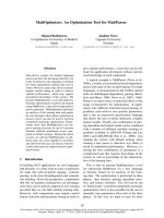
Region representation

To represent a group of histone marks overlapping a
region, these marks are arranged according to their
genomic locations on top of each other and the region.
Then equally-spaced vertical lines are superimposed on
the stack of the marks and the region. The numerical representation of this group of marks is a matrix. A row of
the matrix represents a mark. A column of the matrix
represents a vertical line. If the ith mark intersects the jth
vertical line, the entry i and j in the matrix is 1, otherwise
it is -1. Figure 1 shows the graphical and the numerical

representations of a region and the overlapping marks.
Finally, the two-dimensional matrix is converted to a one
dimensional vector called the epigenetic vector. The number of vertical lines is determined experimentally — 41
and 91 lines were used in our case studies. This number should be adjusted according to the average size of
a region. One may think of this number as the resolution level, the more the vertical lines, the higher the
resolution.
The dotsim function

The dot product of two vectors indicates how close they
are to each other in space. When these vectors are normalized, i.e. each element is divided by the vector norm,


Girgis et al. BMC Bioinformatics (2018) 19:310

Page 3 of 18

result would be [1 0 -1] because the first and the third elements are the same in the three vectors, but the second
element is not.
Hebb’s network

a)

b)
Fig. 1 Representations of a group of chromatin marks overlapping a
region. a Horizontal double lines represent a region of interest.
Horizontal single lines represent the marks. Vertical lines are spaced
equally and bounded by the region. b The intersections between the
marks and the vertical lines are encoded as a matrix where rows
represent the marks and columns represent the vertical lines. If a
vertical line intersects a mark, the corresponding entry in the matrix is

1, otherwise it is -1

the dot product is between 1 and -1. The dotsim function (Eq. 1) normalizes the vectors and calculates their dot
product.
dotsim(x, y) =

y
x
·
x
y

(1)

Here, x and y are vectors; x and y are the norms of
these vectors; the · symbol is the dot product operator. If
the two vectors are very similar to each other, the dotsim
value approaches 1. If the values at the same index of the
two vectors are opposite of each other, i.e. 1 and -1, the
value of dotsim approaches -1.
Data preprocessing

Preprocessing input data is a standard procedure in
machine learning. During this procedure, the noise in the
input data is reduced. First, vectors that consist mainly
of -1’s are removed — a dotsim value of at least 0.8 with the
negative-ones vector. These regions are very likely false
positives. Then, each epigenetics vector is compared to
two other vectors selected randomly from the same set.
The value of an entry in the vector is kept if it is the

same in the three vectors, otherwise it is set to zero. For
example, consider the vector [1 1 -1]. Suppose that the
vectors [1 -1 -1] and [1 -1 -1] were selected randomly. The

Associative learning, also known as Hebbian learning, is
inspired by biology. “When an axon of cell A is near
enough to excite a cell B and repeatedly or persistently
takes part in firing it, some growth process or metabolic
change takes place in one or both cells such that A’s efficiency, as one of the cells firing B, is increased” [62].
Hebb’s artificial neural networks aims at associating two
stimuli: unconditioned and conditioned. After training,
the response to either the conditioned stimulus or the
unconditioned one is the same as the response to both
stimuli combined [63]. In the context of epigenetics, the
unconditioned stimulus, b, is a one-dimensional vector
representing the distributions of histone marks over a
sequence e.g. one tissue-specific enhancer. This vector is
referred to as the epigenetic vector; it is obtained as outlined earlier in this section. The conditioned stimulus is
always the one vector, which include ones in all entries.
We would like to train the network to give a response
when it is given the ones vector, whether or not the epigenetic vector is provided. The response of the network is a
prototype/signature representing the distributions of histone marks over the entire set of genomic locations, e.g.
all enhancers of a specific tissue.
Equations 2 and 3 define how the response of a Hebbian
network is calculated. The training of the network is given
by Eq. 4 [63].
⎧
⎨ +1 if x ≥ 1
if − 1 < x < 1
(2)

satlins(x) = x
⎩
−1 if x ≤ −1
Equation 2 defines a transformation function. This function ensures that the response of the network is similar
to the unconditioned stimulus, i.e. each element of the
response is between 1 and -1. If x is a vector, the function
is applied component wise.
a(b, w, p) = satlins(b + w

p)

(3)

Equation 3 describes how a Hebbian network responds
to the two stimuli (Fig. 2). The response of the network is
transformed using Eq. 2. In Eq. 3, b is the unconditioned
stimulus, e.g. an epigenetic vector; w is the weights vector,
which is the prototype/signature learned so far; and p is
the conditioned stimulus, e.g. the one vector. The operator
represents the component wise multiplication of two
vectors. In the current adaptation, if the network is presented with an epigenetic vector and the one vector, the
response is the sum of the prototype learned so far and the
epigenetic vector. In the absence of the epigenetic vector,


Girgis et al. BMC Bioinformatics (2018) 19:310

Page 4 of 18

regions, a mark with a dotsim value approaching 1 is common in the two signatures. A mark with a dotsim value

approaching -1 has opposite distributions, distinguishing the signatures. Marks with dotsim values approaching
zero do not have consistent distribution(s) in one or both
sets; these marks should not be considered while comparing the two signatures.
Visualizing a chromatin signature

Fig. 2 Unsupervised Hebb’s network: w is the weight vector, which
represents the learned signature; b is an epigentic vector; p is the
ones vector; satlins is the activation/transformation function (Eq. 2); o
is the output of the network; and n is the size of p, b, w, and o

i.e. all-zeros b, the response of the network is the prototype, demonstrating the ability of the network to learn
associations.

Row vectors representing different marks are clustered
according to their similarity to each other. We used hierarchical clustering in grouping marks with similar distributions. The applied hierarchical clustering algorithm
is an iterative bottom-up approach, in which the closest two items/groups are merged at each iteration. The
algorithm requires a pair wise distance function and a
cluster wise distance function. For the pair wise distance function, we utilized the city block function to
determine the distance between two vectors representing
marks. For the group wise distance function, we applied
the weighted pair group method with arithmetic mean
[64]. A digitized image represents the chromatin signature of a genetic element. A one-unit-by-one-unit square
in the image represents an entry in the matrix representing the signature. A row of these squares represents one
mark. The color of a square is a shade between red and
blue if the entry value is less than 1 and greater than -1;
the closer the value to 1 (-1), the closer its color to red
(blue).
Up to this point, we discussed the computational principles of our software tool, HebbPlot. Next, we illustrate the
data used in validating the tool.
Data

wi = wi−1 + α a bi , wi−1 , pi − wi−1

pi

(4)

Equation 4 defines Hebb’s unsupervised learning rule.
Here, wi and wi−1 are the prototype vectors learned in
iterations i and i − 1. The ith pair of unconditioned and
conditioned stimuli is bi and pi . Learning occurs, i.e. the
prototype changes, only when the ith conditioned stimulus, pi , has non-zero components. This is the case here
because pi is always the ones vector. Due to a small α,
which represents the learning and the decay rates, the prototype vector changes a little bit in each iteration when
learning occurs; it moves closer to the response of the
network to the ith pair of stimuli.
Comparing two signatures

One of the main advantages of the proposed method
is that two signatures can be compared quantitatively.
The dotsim function can be applied to the whole epigenetic vector or to the part representing a specific mark.
When comparing the chromatin signatures of two sets of

We used HebbPlot in visualizing chromatin signatures
characterizing multiple genetic elements. Specifically, we
applied HebbPlot to:
•
•
•
•

•
•
•
•
•

Active promoters — 400 base pairs (bp);
Active promoters on the positive strand — 4400 bp;
Active promoters on the negative strand — 4400 bp;
High-CpG active promoters — 400 bp;
Low-CpG active promoters — 400 bp;
Active enhancers — 400 bp and variable size;
Coding regions of active genes — variable size;
Coding regions of inactive genes — variable size; and
Random genomic locations — 1000 bp.

The Roadmap Epigenomics Project provides tens of
marks for more than 100 tissues/cell types [65]. Active
genes were determined according to gene expression levels, which were obtained from the Expression Atlas [66]
and the Roadmap Epigenomics Project [67]. The coding
regions were obtained from the University of California


Girgis et al. BMC Bioinformatics (2018) 19:310

Santa Cruz Genome Browser [68]. The Ensemble genes
for the hg19 human genome assembly were used in this
study. A gene with expression level at least 1 is considered
active, whereas inactive genes have expression levels of 0.
Active promoters are those associated with active genes.

A promoter region is defined as the 400-nucleotides-long
region centered on the transcription start site — except
in one case study, in which the promoter size was 4400
nucleotides. To divide the promoters into high- and lowCpG groups, we calculated the CpG content according to
the method described by Saxonov et al. [69]. Enhancers
active in H1 and IMR90 were obtained from a study by
Rajagopal et al. [54]; this study provides the P300 peaks.
We considered the enhancers to be the 400-nucleotideslong regions centered on the P300 peaks. Regions of
enhancers active in liver, foetal brain, foetal small intestine, left ventricle, lung, and pancreas were obtained
from the Fantom Project [70] — these have variable
sizes.
Once the locations of a genetic element were determined, they are processed further. If the number of
the regions, e.g. tissue-specific enhancers, was more
than 10,000 regions, we uniformly sampled 500 regions
from each chromosome. Each region was expanded by
10% on each end to study how chromatin marks differ from/resemble the surrounding regions. Overlapping
regions, if any, were merged. We used 41 vertical lines for
all case studies except the study comparing the promoters on the positive and the negative strands (91 lines were
used in that study).
In this section, we discussed the computational method
and the data. Next, we apply HebbPlot in six case studies.

Results
Case study: signature of H1-specific enhancers

We studied multiple enhancers active in the H1 cell line
(human embryonic stem cells) obtained from a study conducted by Rajagopal et al. [54]. These enhancers were
detected using P300 ChIP-Seq. This data set contains 5899
enhancers and 27 histone marks. To begin, we plotted
tens of these enhancers; three of these plots are shown in

Fig. 3a–c. No clear signature appears in these plots. After
that, a HebbPlot representing the signature of H1-specific
enhancers was generated (Fig. 3d) using an unsupervised
hebbian network. For comparison purposes, we generated
a conventional plot (Fig. 3e). To generate this plot, the
middle points of all regions are aligned. Then the intensity
of a mark at each nucleotide is calculated as the number
of times the mark is present at this nucleotide. Figure 3f
shows the average plot of the epigenetic vectors of all
regions. Finally, we clustered all of the epigenetic vectors
(except now the vector is filled row-wise not columnwise from the matrix) using hierarchical clustering
(Fig. 4).

Page 5 of 18

The HebbPlot shows four zones representing the absent
marks, and the present ones with different confidence
levels. For example, the top zone shows four marks
(H2A.Z, H4K8ac, H3K36me3, and H4K20me1) that are
absent from the H1 enhancers. The second zone from
the top shows marks with very weak intensities including H3K9me3, H3K27me3, H3K79me2, and H3K79me1.
The third zone has an ellipse, which is cooler — less
red — than the surrounding area, implying that the signals
of the marks within the ellipse are weaker than the surroundings. The bottom zone shows two marks (H3K4me1
and H3K4me2) that are present around these enhancers
consistently.
In the upper part of the conventional plot, a large number of marks show depressions near the middle of the plot.
However, these depressions are mixed with few peaks,
making them hard to view. These depressions correspond
to the fragments near the centers of the individual plots

and the ellipse in the middle of the third zone of the
HebbPlot. The ellipse in the third zone of the HebbPlot
captures this pattern much better than the conventional
plot. Further, marks with similar intensities overlap each
other in the conventional plot, obstructing one another —
the more the marks, the worse the obstruction. To illustrate, this figure was generated using 27 marks; there are
about 100 known histone marks; therefore, using these
conventional figures may not be the best way to visualize the intensities of a large number of marks. In contrast,
HebbPlot can handle a large number of marks efficiently
because each mark has its own row. Furthermore, no
noise-removal process was applied while constructing the
conventional figure. In contrast, only regions, or subregions, that are recognized by the network contribute to
the HebbPlot.
The average plot shows similar zones to the ones
shown in the HebbPlot; however, they are very fuzzy.
One area of comparison is the ellipse in the third
zone. In the average plot, this ellipse is spanning almost
the entire zone, implying that these marks are weakly
present around the 400-nucleotides-long enhancers. In
contrast, the ellipse is smaller in the HebbPlot, suggesting that these marks are weakly present around the
center of these enhancers, not the entire regions. The
differences between the average plot and the HebbPlot
are due to the network selectivity to which regions or
sub-regions are utilized in learning the signature. Not
all regions, or sub-regions, contribute to the learned
signature. Regions and sub-regions that cause the network to fire, i.e. they are recognized by the network,
contribute to the learned signatures (Eqs. 2, 3, and 4).
These results suggest that HebbPlot produces more
accurate and more biologically relevant results.
Hierarchical clustering has been a common method

in analyzing and visualizing histone data. This method


Girgis et al. BMC Bioinformatics (2018) 19:310

Page 6 of 18

a)

b)

c)

e)

d)

f)

Fig. 3 Retrieving the chromatin signature of the H1-specific enhancers. Three examples of enhancers are shown in Parts a–c. A row in one of these
plots represents the distribution of one mark around a region; red (blue) color indicates the presence (absence) of a mark. It is hard to see a
common pattern in these three examples. The signature learned by the Hebbian network is captured by the HebbPlot shown in Part d. A row in the
HebbPlot represents the distribution of a mark around all enhancers in the data set. The closer the color to red, the higher the certainty of the
presence of a mark around the corresponding sub-region. The HebbPlot is characterized by four zones. The top most zone represents chromatin
marks that are absent from the enhancer regions, whereas the next three zones represent the present marks with increasing certainty. A
conventional plot of the intensities of all marks around every region in the data set in shown in Part e. Many marks show depressions near the
center of the plot; however, some peaks are mixed with these depressions in the conventional plot. In contrast, these depressions correspond to the
ellipse in the middle of the third zone of the HebbPlot. This ellipse is very clear. Further, marks of similar intensities obstruct one another in the
conventional plot. This is not the case with HebbPlot because every mark is represented by a separate row. An average plot is displayed in Part f.
This plot shows a similar — but fuzzy — pattern to the one found by the network

is very useful in identifying the number of signatures
present in the data, but the displayed clusters, which represent the found signatures, are not easy to be interpreted.
On the other hand, the current version of HebbPlot can
characterize only one signature — not multiple signa-

tures as the hierarchical clustering. However, a HebbPlot
is intuitive and can be easily interpreted. These two methods can be used together when the data contains multiple
signatures, which does not appear to be the situation in
this case study. First, a user may use hierarchical clus-


Girgis et al. BMC Bioinformatics (2018) 19:310

Page 7 of 18

Fig. 4 Hierarchical clustering of histone marks around 5899 H1-specific enhancers. The epigenetic vectors, except they are filled row-wise not
column-wise, are clustered. This figure shows that certain marks have clear consistent pattern around these regions. However, the specific signature
of these marks is not easily interpreted

tering, or any clustering algorithm, to identify different
clusters. Then the user can generate a HebbPlot from each
cluster.
In sum, HebbPlot has advantages to plots based on the
average, conventional plots, and plots based on clustering
the underlying histone data.
Next, we study the signatures of enhancers, promoters,
and coding regions of active genes in the liver.
Case study: histone signatures of different active elements
in liver

Seven histone marks of the human liver epigenome are
available. We obtained 5005 enhancers, 13,688 promoters,
and 12,484 coding regions of active genes in liver. In
addition, we selected 10,000 locations sampled uniformly
from all chromosomes of the human genome as controls.
Then we trained four Hebbian networks to learn the chromatin signature of each genetic element. As expected,
the HebbPlot representing the random genomic locations displays a deep-blue box (not shown), indicating
that no chromatin mark is distributed consistently around
these regions. Figure 5 shows three HebbPlots of the
enhancers, the promoters, and the coding regions. The
three signatures have similarities and differences. Two

marks, H3K9me3 and H3K27me3, are absent from the
three signatures. However, the three signatures are distinguishable. H3K36me3 is the strongest mark of the coding
regions, whereas it is absent from the promoters and the
enhancers. On the other hand, H3K27ac is the strongest
mark on the promoters and the enhancers, but almost
absent from the coding regions. H3K4me1 is stronger
than H3K4me3 around the enhancers, but H3K4me3 is
stronger than H3K4me1 around the promoters. Both of
these marks are absent from the coding regions. These
plots demonstrate that HebbPlot is able to learn the chromatin signature from a group of regions with the same
function. In addition, the chromatin signatures of the
promoters, the enhancers, and the coding regions have
similarities and differences.
Case study: The directional signature of active promoters

Because promoters are upstream from their genes,
some marks may indicate the direction of the transcription. To determine whether or not marks have

direction, active promoters (4400 nucleotides long)
were separated according to the positive and the
negative strands into two groups. We trained two
Hebbian networks to learn the chromatin signatures


Girgis et al. BMC Bioinformatics (2018) 19:310

a)

Page 8 of 18

b)

c)

Fig. 5 Liver chromatin signatures representing a active enhancers, b active promoters, and c coding regions of active genes. The three signatures
have similarities and differences. They are similar in that H3K9me3 and H3K27me3 are absent from all of them. H3K36me3 is the strongest mark of
coding regions, whereas H3K27ac is the strongest mark of promoters and enhancers. H3K4me1 is stronger than H3K4me3 in enhancers; this relation
is reversed in promoters, where H3K4me1 is weak around transcription start sites

of active promoters on the positive and the negative
strands. Figure 6 shows the HebbPlots of the positive
and the negative promoters active in HeLa-S3 cervical carcinoma cell line. These two plots are mirror
images of each other, showing H3K36me3, H3K79me2,
H3K4(me1,me2,me3), H3K27ac, and H3K9ac stretching
more downstream than upstream and H2A.Z in the
opposite direction.
Then we generated HebbPlots for the positive (Additional
file 1) and the negative (Additional file 2) promoters of 57

tissues, for which we know their gene expression levels.
The directional signature of promoters is very consistent
in these tissues. After that, we determined quantitatively
which marks having directional preferences in the 57
tissues/cell types. To determine directional marks, the
learned prototype of a mark over the upstream third of
the promoter region was compared to the prototype of
the same mark over the downstream third. If the dotsim

a)

value between the two prototypes is negative, this mark
is considered directional. We list the results in Table 1.
H3K4me3 and H3K79me2 show directional preferences
in 72% and 71% of the tissues. Additional 12 marks show
directional preferences in 50–70% of the tissues. These
results indicate that active promoters have a directional
chromatin signature.
Case study: The signatures of high- and low-CpG promoters

It has been reported in the literature that the chromatin
signature of high-CpG promoters is different from the
signature of low-CpG promoters [47]. In this case study,
we used HebbPlot to demonstrate this phenomenon. To
this end, we divided promoters active in skeletal muscle myoblasts cells into high-CpG and low-CpG groups
using the method proposed by Saxonov et al. [69]. The
high-CpG group consists of 12825 promoters and the
low-CpG group consists of 2712 promoters. After that,

b)

Fig. 6 HebbPlots of active promoters in HeLa-S3 cervical carcinoma cell line. These promoters were separated into two groups according to their
strands. The size of a promoter is 4400 nucloetides. The two HebbPlots of the promoters on the positive and the negative strands are mirror images
of each other. Multiple marks including H3K36me3, H3K79me2, H3K4me1, H2A.Z, H3K27ac, H3K9ac, H3K4me3, and H3K4me2 are distributed in a
direction specific way. H2A.Z tends to stretch upstream, whereas the rest of these directional marks tend to stretch downstream from the promoters
toward their coding regions. a Promoters on the positive strand, b Promoters on the negative strand


Girgis et al. BMC Bioinformatics (2018) 19:310

Page 9 of 18

Table 1 Promoters — 4400 nucleotides long — were separated
according to the strand to positive and negative groups
Mark

Known

Directional

Percentage (%)

H3K4me3

57

41

72

H3K79me2

14

10

71

H3K4me2

16

11

69

H2AK5ac

6

4

67

H3K18ac

6

4

67

H2A.Z

14

9

64

H3K4me1

57

35

61

H2BK12ac

5

3

60

H3K14ac

5

3

60

H3K9ac

24

13

54

H2BK5ac

6

3

50

H3K23ac

6

3

50

H3K4ac

6

3

50

H3K79me1

6

3

50

H3K27ac

49

22

45

H4K91ac

5

2

40

H4K8ac

6

2

33

H2BK120ac

6

1

17

H4K20me1

12

2

17

H3K36me3

57

6

11

Mark vectors over the upstream and the downstream thirds of the promoters on
the positive strand were compared. A mark is considered directional if these two
vectors have a negative dotsim value. The number of cell types, for which a mark
was determined, is listed under “Known.” The number of cell types, in which a mark
has directional preference around the promoter regions, is listed under “Directional.”
The percentage of times a mark showed directional preference is listed under
“Percentage.” Only marks determined for at least five tissues were considered

a)

we generated two HebbPlots from these two groups
(Fig. 7).
The two signatures are very different. The high-CpG
HebbPlot has more red bands than that of the low-CpG
group, indicating that these histone marks are consistently
distributed around the high-CpG promoters. Few marks
distinguish the two signatures. The high-CpG group is
characterized by the presence of H3K4me3, H3K9ac, and
H3K27ac, which are very weak or absent from the lowCpG promoters. The low-CpG group is characterized by
the presence of H3K36me3, which is absent from the
high-CpG promoters. These two signatures are different
from those reported by Karlic et al. [47]. Two factors may
cause these differences. First, the size of the promoter
region differs between the two studies. In our study, the
size of the promoter is 400 base pairs, while it is defined
as 3500 base pairs long (−500 to +3000) in the other
study. This longer region is likely to overlap with untranslated and coding regions, whereas it is less likely that
the 400-base-pairs-long promoter to overlap with these

regions. The second factor is that the other study focuses
on the correlation between histone marks and expression
level, whereas the main purpose of our case study is
to visualize the signature of the promoters. Therefore,
our definition is more relevant to the visualization
task.
Next, we performed quantitative comparisons to see if
these marks are distributed differently around high- and
low-CpG promoters in a consistent way in the 57 tissues.
A main advantage of HebbPlots is that they can be compared quantitatively. HebbPlots were generated from the
high-CpG promoters (Additional file 3) and the low-CpG
promoters (Additional file 4) in the 57 cell types/tissues.
We calculated the average dotsim of the two vectors representing a mark around high- and low-CpG promoters

b)

Fig. 7 Promoters active in skeletal muscle myoblasts cells were separated into high- and low-CpG groups. A HebbPlot was generated from each
group. Clearly, the two signatures are different. Specifically, H3K4me3, H3K9ac, and H3K27ac are present around the high-CpG promoters, whereas
they are very weak or absent from the low-CpG promoters. In contrast, H3K36me3 is absent from the high group, but present around the low-CpG
promoters. In general, marks present around the high-CpG promoters are stronger than those present around the low-CpG ones. a High-CpG
promoters, b Low-CpG promoters


Girgis et al. BMC Bioinformatics (2018) 19:310

Page 10 of 18

in the 57 tissues. Table 2 shows the results. These results
confirm that H3K4me3, H3K9ac, and H3K27ac are consistently different around high- and low-CpG promoters
(average dotsim value < -0.5). However, H3K36me3 is not

different overall (average dotsim value of 0.65). Further,
this analysis reveals that H2BK120ac and H4K91ac are
also distributed differently around the two groups (average dotsim < -0.5); their signals are stronger around the
high-CpG group than the low group.
In sum, the chromatin signatures of high- and low-CpG
promoters are different. Five marks are present around
high-CpG promoters, whereas they are absent from or
very weak around low-CpG promoters.
Case study: signature of active enhancers

Here, we demonstrate HebbPlot’s applicability to visualizing the chromatin signatures of enhancers in multiple
tissues. To this end, we collected active enhancers from
two sources. Enhancers active in H1 (5899 regions) and
Table 2 High-CpG promoters have a different signature from
that of low-CpG promoters
Mark

Known

Average dotsim

H3K4me3

57

-0.98452

H3K9ac

24

-0.82137

H3K27ac

49

-0.72655

H2BK120ac

6

-0.53278

H4K91ac

5

-0.48083

H3K4me2

16

-0.33263

H3K23ac

6

-0.32737

H2A.Z

14

-0.27855

H2BK12ac

5

-0.20927

H2BK5ac

6

-0.15632

H3K4ac

6

-0.15405

H4K8ac

6

-0.12716

H2AK5ac

6

-0.11522

H3K14ac

5

-0.03981

H3K18ac

6

0.14699

H3K4me1

57

0.24636

H3K79me1

6

0.35168

H3K79me2

14

0.62139

H3K36me3

57

0.65545

H4K20me1

12

0.82929

H3K27me3

57

0.92651

H3K9me3

57

0.97729

Active promoters in 57 tissues/cell types were divided into two groups according to
their CpG contents. Then two networks were trained on the two groups, producing
two signatures for each tissue/cell type. The two signatures of a mark in the same
tissue were compared using the dotsim function. The average dotsim values are
listed under “Average dotsim.” Not all marks were determined for all tissues. The
number of tissues/cell types, for which a mark was determined, is listed under the
column titled “Known”

IMR90 (14073 regions) were obtained from a study by
Rajagopal et al. [54]. Enhancers active in other six tissues
were obtained from the Fantom Project. We selected these
tissues because they were common to the Fantom and the
Roadmap Epigenomics Projects. These enhancers include
5005 regions for liver, 1476 regions for foetal brain, 5991
regions for foetal small intestine, 1619 regions for left
ventricle, 11003 regions for lung, and 2225 regions for
pancreas.
Next, we generated a HebbPlot from the enhancers of
each tissue/cell type (Additional file 5). Figure 8 show
the eight HebbPlots. The HebbPlots of the enhancers
active in H1 and IMR90, for which more than 20
marks have been determined, show that multiple marks
are abundant around enhancer regions. Similar to what
has been reported in the literature, we observed that
H3K4me1 is usually stronger than H3K4me3 around
enhancers [71]; however there are some exceptions, e.g.
foetal brain and lung. H3K27ac and H3K9ac are also

present around enhancers, but H3K9me3, H3K27me3,
and H3K36me3 are very weak or absent from enhancers.
Further, these HebbPlots suggest that the chromatin signatures of enhancers active in different tissues are similar;
however, they are not identical. For example, H3K27ac is
the predominant mark around lung enhancers; H3K4me1
and H3K4me3 are also present, but their signals are
weak. In contrast, H3K27ac and H3K4me1 have comparable signals, which are stronger than H3K4me3, around
enhancers of foetal small intestine.
Case study: signatures of coding regions of active and
inactive genes

Multiple studies indicate that histone marks are associated with gene expression levels [52, 72, 73]. In this
case study, we demonstrate the usefulness of HebbPlot in
identifying histone marks associated with high and low
expression levels. Genes were divided into nine groups
based on their expression levels in IMR90 (Additional
file 6). A HebbPlot was generated from the coding regions
of each of these groups (Fig. 9). We found that H3K36me3
and H3K79me1 mark the top two groups. On the lowest six groups, which represent coding regions of inactive
genes, these two marks are absent, whereas H3K27me3 is
present. H2A.Z is present in all groups. Generally, the heat
— demonstrated by red — of a HebbPlot decreases as the
gene expression levels decrease. These results show that
HebbPlot can help with identifying marks associated with
coding regions of active and inactive genes.
After that, we asked whether these marks consistently mark active and inactive coding regions in other
tissues/cell types. To answer this question, we generated
HebbPlots of coding regions of active (Additional file 7)
and inactive (Additional file 8) genes in the 57 tissues/cell
types. We calculated the average dotsim values of each

Girgis et al. BMC Bioinformatics (2018) 19:310

Page 11 of 18

a)

c)

f)

b)

d)

e)

g)

h)

Fig. 8 Signatures of active enhancers. Enhancers were collected from a study by Rajagopal et al. [54] and from the Fantom Project. A HebbPlot was
generated from the enhancers of each tissue. The HebbPlots of H1 and IMR90, for which more than 20 marks are known, show that several marks
are present around active enhancers. Usually, H3K4me1 has a stronger signal around enhancers than H3K4me3; however there are some
exceptions, e.g. foetal brain. H3K9ac and H3K27ac are present around enhancers, but H3K9me3, H3K27me3, and H3K36me3 are very weak or absent
from enhancers. These plots show that chromatin signatures of enhancers active in different tissues are similar, but not identical. a H1, b IMR90,
c Liver, d Foetal brain, e Foetal small intestine, f Left ventricle, g Lung, h pancreas

mark in the two signatures in the tissues/cell types, for

which this mark has been determined. H3K36me3 and
H3K79me1 are very different around active and inactive coding regions (average dotsim: -0.86 and -0.64).
H3K27me3 is also different (average dotsim: 0.44), but the
difference is not as strong as H3K36me3 and H3K79me1.
After that we asked which other marks are distributed
differently around coding regions of active and inactive
genes. We found that H3K79me2 consistently marks

active coding regions (average dotsim: -0.38). Additionally, we found H4K8ac weakly marks active coding regions
(average dotsim: 0.45). Regarding the marks of inactive
coding regions, H4K12ac was found to mark these regions
(dotsim: -0.67) — this mark has been determined for one
tissue only. H4K14ac and H2AK5ac were found to weakly
mark inactive coding regions (average dotsim: 0.34 and
0.46). Generally, the active marks are stronger than the
inactive marks.


Girgis et al. BMC Bioinformatics (2018) 19:310

Page 12 of 18

a)

b)

c)

d)

e)

f)

g)

h)

i)

Fig. 9 Histone marks are highly associated with gene expression levels in IMR90. Genes were divided into nine groups according to their expression
levels. A HebbPlot was generated from the coding regions of each group. In general, a HebbPlot cools down — becomes bluer — as the expression
level decreases. The more red a row is, the more consistent its mark is distributed around the set of regions. H3K36me3 and H3K79me1 mark the
coding regions of active genes in IMR90, whereas the repressive modification, H3K27me3, marks the inactive coding regions. H2A.Z is ubiquitous.
a First group, b Second group, c Third group, d Fourth group, e Fifth group, f Sixth group, g Seventh group, h Eighth group, i Ninth group

Toward a functional catalog of histone marks

Table 3 shows a summary of the findings of this study.
Up to this point, we demonstrated the usefulness
of HebbPlot in six case studies. Next, we discuss the
similarities and the differences between HebbPlot and
other visualization tools.

Discussion
Comparison to related tools

Visualization of chromatin marks and their associations
with thousands of elements active in a specific cell type
is critical to deciphering the function(s) of these marks.

Extracting trends and patterns by mere inspection is
essentially impossible given that there are more than 100
known chromatin marks and thousands of sequences. As
such, it is vital for biologists to have visualization tools
to aid in these tasks. To this end, several tools — Chromatra, ChAsE, and DGW — have been developed. In
addition, we have created our own visualization technique, HebbPlot. Unlike the other three tools, which cluster genomic regions according to histone modifications,
HebbPlot uses an artificial neural network to summarize the data in a form that is convenient for biologists.
The following is a brief discussion about HebbPlot and


Girgis et al. BMC Bioinformatics (2018) 19:310

Page 13 of 18

Table 3 A catalog of functions of histone marks in this study
Mark

Function

Literature support

H2A.Z

Directional around promoters stretching upstream.

Associated with trascription start sites [39] and
promoters [36].

H2AK5ac

Directional around promoters stretching downstream
and weakly associated with coding regions of inactive
genes.

–

H2BK5ac

Directional around promoters stretching downstream.

Associated with promoters [36, 47].

H2BK12ac

Directional around promoters stretching downstream.

–

H2BK120ac

Associated with high-CpG promoters.

Associated with promoters and CpG islands [36].

H3K4ac

Directional around promoters stretching downstream.

Associated with promoters [36].

H3K4me1

Directional around promoters stretching downstream,
absent around transcription start sites, and associated
with enhancers.

Associated with enhancers [37, 39].

H3K4me2

Directional around promoters stretching downstream
and associated with enhancers.

Associated with promoters [74] and enhancers [36].

H3K4me3

Directional around promoters stretching downstream,
associated with high-CpG promoters, and associated
with enhancers — usually weaker than H3K4me1.

Associated with trascription start sites [39], promoters
[36, 37, 74, 75], CpG islands [36], and enhancers
[36, 39].

H3K8ac

Weakly associated with coding regions of active genes.

–

H3K9ac

Directional around promoters stretching downstream,
associated with high-CpG promoters, and associated
with enhancers.

Associated with promoters [74] and CpG islands [36].

H3K9me3

Weakly associated with coding regions of inactive
genes, and very weak/absent from enhancers, and very
weak/absent from promoters.

Associate with “repressed regions” [37, 72].

H3K14ac

Directional around promoters stretching downstream
and weakly associated with coding regions of inactive
genes.

–

H3K18ac

Directional around promoters stretching downstream.

–

H3K23ac

Directional around promoters stretching downstream.

–

H3K27ac

Associated with high-CpG promoters and enhancers.

Associated with trascription start sites [39], promoters
[36, 74], high-CpG promoters [47], CpG islands [36],
and enhancers [36, 39].

H3K27me3

Weakly associated with coding regions of inactive
genes, very weak/absent from enhancers, and very
weak/absent from promoters.

“Repressive mark” [37, 72, 75].

H3K36me3

Associated with coding regions and very weak/absent
from enhancers.

Associated with and directional around “transcriped

gene bodies" [75]; associated with “transcribed
regions” [37] and highly expressed genes [72].

H3K79me1

Directional around promoters stretching downstream
and associated with coding regions of active genes.

Associated with promoters active in CD4+ [47] and
“transcribed regions” [37].

H3K79me2

Directional around promoters stretching downstream
and associated with coding regions of active genes.

Associated with “transcribed regions” [37].

H4K12ac

Associated with coding regions of inactive genes — this
mark is known in one tissue only.

–

H4K91ac

Associated with high-CpG promoters.

Associated with promoters [36] and CpG islands [36].

its characteristics that differ from the aforementioned
utilities.
Chromatra is a visualization tool that displays chromatin mark enrichment of subregions of each of the input
regions. Since it is a plug-in for the well-supported Galaxy
platform, it is simple for a user to add it to his or her

list of tools. Additionally, this tool is comprised of two
modules for chromatin mark analysis. The first module
calculates the enrichment scores of a given chromatin
mark on a given set of genomic locations of interest. The
second module, while similar to the first, adds the additional functionality of clustering the results by additional


Girgis et al. BMC Bioinformatics (2018) 19:310

parameters, e.g. gene expression levels. All results of these
modules are then projected onto a heat map, which can
be exported for further research. While Chromatra’s easeof-use and versatility are common characteristics between
it and HebbPlot, HebbPlot takes a dramatically different
approach to how it clusters data. Whereas Chromatra
handles enrichment levels in genomic regions of variable
length through binning, HebbPlot will extract the same
number of points for any region. HebbPlot will then utilize an artificial neural network to derive a representative
pattern for the chromatin marks across all of the points
in every region. Our tool proceeds to cluster the patterns
for each chromatin mark according to their similarity to
each other, and then produces a heat map of the results.
Therefore, rather than evaluate genomic regions that have
been mapped to chromatin marks, HebbPlot summarizes

the distribution of each chromatin mark across a “representative” region. This allows researchers to only have to
view one heat map before acquiring a solid understanding
of how the histone modifications are represented across
the regions.
ChAsE and HebbPlot have their basis in displaying
information clearly and easily to the user. Their design
philosophy is rooted in the fact that many visualization
tools demand a high amount of technical knowledge that
is unreasonable to expect from researchers. With this
said, HebbPlot and ChAsE also diverge significantly in
how they cluster the input and how they present their
results. Similar to Chromatra, ChAsE will cluster regions
together based on the abundance of chromatin marks (or
any genomic area of interest) in each region. Afterwards,
ChAsE allows the user the flexibility to inspect the clusters
further via methods like K-Means clustering and signal
queries. HebbPlot, as explained before, samples a fixed
number of points in each given region of interest. These
samples, and the overlapping marks, are then processed by
an artificial neural network to determine a motif for each
histone modification that is illustrative of its distribution
in all given regions. The motifs for each considered modification is then clustered in a hierarchy so that all modifications of similar enrichment levels are placed together. A
digital image of this detailed clustering is then produced,
providing researchers with a way to quickly understand
how histone marks are distributed across a representative
regions.
DGW is a tool that consists of two modules. The first is
an alignment and clustering module, whereas the second
is a visualizer for the results. DGW is designed to “rescale
and align” the histone marks of genomic regions (such as

transcription start sites and splicing sites). Additionally,
it hierarchically clusters the aligned marks into distinct
groups. Regarding the visualization module, DGW creates
heat maps and dendrograms of chromatin marks of a set of
genomic locations. There are several notable similarities

Page 14 of 18

and differences between DGW and HebbPlot. HebbPlot
is similar to DGW in that it scales the regions. However,
HebbPlot implements it using a different idea. Specifically,
HebbPlot samples a fixed number of equally spaced points
from each region regardless of the region length. HebbPlot
learns a general pattern of chromatin marks summarizing all of the input regions as one representative region.
Unlike DGW, hebbPlot does not cluster the input regions
based on the distribution of a mark. Hierarchical clustering is utilized in HebbPlot not to cluster the regions
according to the enrichment of a mark, but to cluster all
marks according to their distributions around the representative region. The amount of details produced by
DGW can be inappropriate in the presence a large number
of marks and regions. HebbPlot on the other hand, is built
specifically to make large amounts of data manageable
and meaningful for biologists through its summarization
technique.
Our comparisons regarding these four tools makes it
clear that the advantages provided by HebbPlot are not
well represented among related tools. There are numerous
tools for clustering regions according to the abundance
of chromatin marks, but besides conventional plots, there
are hardly any techniques for determining the patterns
of marks across all regions. This means it is important

for HebbPlot to coexist among other popular visualization
tools. Its unique and concise summarization of data is vital
to evaluating a large number of chromatin signals across
thousands of regions. This is not to say that the level of
description provided by other tools is not useful. Indeed,
biologists need to be able to see the specific results that
other utilities facilitate. However, what HebbPlot offers is
a look at the “big picture” of the data.
Selection of region size in our case studies

Two reasons led us to choose 400 base pairs (bp) as the
size of enhancers and promoters in some case studies.
Frist, the average size of the enhancers obtained from the
Fantom project is around 400 bp. In the Fantom project,
the whole region was determined according to eRNA
(enhancer RNA) not only the peak as with the P300. Second, this size was necessary in some case studies; for
example, to make sure that the promoter signature is as
accurate as possible, we needed to limit the size to 400
bp to minimize the overlap with untranslated and coding regions. However, in other case studies such as the
one involving the directionality of the promoter signature, we used 4400 bp to see outside the promoter regions.
Additionally, HebbPlot can process regions of any size.
We have conducted some experiments using sizes ranging from 200 bp to 5000 bp. See Additional file 9: Figure
S1 and Additional file 10: Figure S2. The two figures suggest that 400 bp are reasonable to show the signature of
promoters and enhancers active in H1.


Girgis et al. BMC Bioinformatics (2018) 19:310

Page 15 of 18

Handling regions with variable sizes

Handing regions of the same size, e.g. promoters, is
straight forward; however, handling regions of variable
sizes, e.g. coding regions, requires rescaling. One drawback of conventional plots is that they do not account
for length difference, resulting in an artificial peak(s) due
to small regions. Our approach to sample fixed number of points from each region in a data set works on
regions that have variable or similar lengths and is supported by the histone code hypothesis. If histone marks
are distributed in a similar way around regions that have
the same function, then sampling equally-spaced points
from these regions should capture the histone signature.
In some sense, this is a rescaling process. To illustrate,
imagine three triangles of different sizes (Fig. 10) representing the distributions of chromatin marks around three
regions. If we take three equally-spaced samples from
each region then these samples should capture a simple,
yet accurate, representation of the chromatin signature —
low signal, high signal, followed by low signal. Using more
samples should result in a better representation of a signature. In sum, our approach, which is supported by the
histone code hypothesis, allows for extracting signatures
from regions with variable or fixed lengths.

Conclusions
In this manuscript, we described a new software tool,
HebbPlot, for learning and visualizing the chromatin signature of a genetic element. HebbPlot produces an image
that can be interpreted easily. Signatures learned by HebbPlot can be compared quantitatively. We validated HebbPlot in six case studies using 57 human tissues and cell
types. The results of these case studies are novel or confirming to previously reported results in the literature,
indicating the accuracy of HebbPlot. We found that active
promoters have a directional chromatin signature; specifically, H3K4me3 and H3K79me2 tend to stretch downstream, whereas H2A.Z tends to stretch upstream. Our
results confirm that high-CpG and low-CpG promoters
have different chromatin signatures. When we compared

the signatures of enhancers active in eight tissues/cell
types, we found that they are similar, but not identical.
Contrasting the signatures of coding regions of active
and inactive genes revealed that certain modifications—
H3K36me3, H3K79(me1,me2), and H4K8ac — mark
active coding regions, whereas different modifications —
H4K12ac, H3K14ac, H3K27me3 and H2AK5ac — mark
coding regions of inactive genes. Our study resulted in a
visual catalog of chromatin signatures of multiple genetic
elements in 57 human tissues and cell types. Further, we
made a progress toward a functional catalog of more than
20 histone marks. Finally, HebbPlot is a general tool that
can be applied to a large number of studies, facilitating the
understanding of the histone code.

Fig. 10 The advantage of HebbPlot is clear when looking at
variable-sized regions. Each triangle represents the distributions of
chromatin marks around a region. The three equally-spaced samples
(X) obtained from each region give a rise to a pattern of low signal
(-1), high signal (1), and low signal (-1). Conventional plots wouldn’t
detect this pattern because of the differences in length. Hebbplot,
however, will rescale these triangles and present the correct signature

Availability and requirements
The source code (Perl and Matlab) is available as Additional
file 11.
Project name: HebbPlot.
Project home page: informaticsToolsmith/HebbPlot
Operating system(s): UNIX/Linux/Mac.
Programming language: Perl and Matlab.

Girgis et al. BMC Bioinformatics (2018) 19:310

Other requirements: Matlab Statistics and Machine
Learning Toolbox and Bedtools (d thedocs.io/en/latest/).
License: Creative Commons license (attribution + noncommercial + no derivative works).
Any restrictions to use by non-academics: License
needed.

Additional files
Additional file 1: HebbPlots of active promoters on the positive strand.
This compressed file (.tar.gz) includes HebbPlots of promoters on the
positive strand active in 57 tissues/cell types. (TAR 2949 kb)
Additional file 2: HebbPlots of active promoters on the negative strand.
This compressed file (.tar.gz) includes HebbPlots of promoters on the
negative strand active in 57 tissues/cell types. (TAR 2952 kb)
Additional file 3: HebbPlots of high-CpG promoters. This compressed file
(.tar.gz) includes HebbPlots of high-CpG promoters active in 57 tissues/cell
types. (TAR 2654 kb)
Additional file 4: HebbPlots of low-CpG promoters. This compressed file
(.tar.gz) includes HebbPlots of low-CpG promoters active in 57 tissues/cell
types. (TAR 2971 kb)
Additional file 5: HebbPlots of active enhancers. This compressed file
(.tar.gz) includes HebbPlots of enhancers active in eight tissues/cell types.
(TAR 439 kb)
Additional file 6: Gene identifiers. This compressed file (.tar.gz) includes
identifiers of nine groups of genes divided according to their gene
expression levels in IMR90. (TAR 428 kb)
Additional file 7: HebbPlots of coding regions of active genes. This

compressed file (.tar.gz) includes HebbPlots of genes active in 57
tissues/cell types. (TAR 2696 kb)
Additional file 8: HebbPlots of coding regions of inactive genes. This
compressed file (.tar.gz) includes HebbPlots of genes inactive in 57
tissues/cell types. (TAR 2715 kb)
Additional file 9: Figure S1. HebbPlots of enhancers specific to H1 cell
line. These plots were generated from enhancers with different sizes. Each
HebbPlot was generated from a set of enhancers, all of which have the
same size and are centered on the P300 peaks. (PDF 4881 kb)
Additional file 10: Figure S2. HebbPlots of promoters active in H1 cell
line. These plots were generated from promoters with different sizes. Each
HebbPlot was generated from a set of promoters, all of which have the
same size and are centered on the transcription start sites. (PDF 5010 kb)
Additional file 11: HebbPlot Software. This compressed file (.tar.gz)
includes the source code (Matlab and Perl) of HebbPlot. (TAR 15 kb)
Abbreviations
bp: Base pairs
Acknowledgements
The authors would like to thank Michael Buck, Associate Professor of
biochemistry at the State University of New York at Buffalo, for useful
discussions. We are grateful to the anonymous reviewers for their comments
and suggestions, which improved the software as well as this manuscript.
Funding
This research was supported by internal funds provided by the College of
Engineering and Natural Sciences and the Faculty Research Grant Program at
the University of Tulsa. The funding body did not play any roles in the design
of the study and collection, analysis, and interpretation of data and in writing
the manuscript.
Availability of data and materials
The source code of HebbPlot and data produced in the case studies are

available as Additional files 1–9.

Page 16 of 18

Authors’ contributions
HZG designed the software and the case studies, implemented the neural
network, and wrote the manuscript. AV coded the software, processed the
data, and wrote the manuscript. ZER processed the data and wrote the
manuscript. All authors read and approved the final version of the manuscript.
Ethics approval and consent to participate
Not applicable.
Consent for publication
Not applicable.
Competing interests
The authors declare that they have no competing interests.

Publisher’s Note
Springer Nature remains neutral with regard to jurisdictional claims in
published maps and institutional affiliations.
Received: 12 December 2017 Accepted: 14 August 2018

References
1. Carey N. The Epigenetics Revolution: How Modern Biology Is Rewriting
Our Understanding of Genetics, Disease, and Inheritance. New York
Chichester, West Sussex: Columbia University Press;
2012, p. 206.
2. Lewis JD, Meehan RR, Henzel WJ, Maurer-Fogy I, Jeppesen P, Klein F,
Bird A. Purification, sequence, and cellular localization of a novel
chromosomal protein that binds to methylated DNA. Cell. 1992;69(6):
905–14.

3. Jenuwein T, Allis CD. Translating the histone code. Science.
2001;293(5532):1074–80.
4. Kouzarides T. Chromatin modifications and their function. Cell.
2007;128(4):693–705.
5. Whitelaw NC, Chong S, Morgan DK, Nestor C, Bruxner TJ, Ashe A,
Lambley E, Meehan R, Whitelaw E. Reduced levels of two modifiers of
epigenetic gene silencing, Dnmt3a and Trim28, cause increased
phenotypic noise. Genome Biol.
2010;11(11):R111.
6. Carone BR, Fauquier L, Habib N, Shea JM, Hart CE, Li R, Bock C, Li C, Gu H,
Zamore PD, Meissner A, Weng Z, Hofmann HA, Friedman N, Rando OJ.
Paternally induced transgenerational environmental reprogramming of
metabolic gene expression in mammals. Cell. 2010;143(7):1084–96.
7. Ng S-F, Lin RCY, Laybutt DR, Barres R, Owens JA, Morris MJ. Chronic
high-fat diet in fathers programs β-cell dysfunction in female rat
offspring. Nature. 2010;467(7318):963–6.
8. Anway MD, Cupp AS, Uzumcu M, Skinner MK. Epigenetic
transgenerational actions of endocrine disruptors and male fertility.
Science. 2005;308(5727):1466–9.
9. Guerrero-Bosagna C, Settles M, Lucker B, Skinner MK. Epigenetic
transgenerational actions of vinclozolin on promoter regions of the
sperm epigenome. PLoS ONE. 2010;5(9):1–17.
10. Fraga MF, Ballestar E, Paz MF, Ropero S, Setien F, Ballestar ML,
Heine-Suñer D, Cigudosa JC, Urioste M, Benitez J, Boix-Chornet M,
Sanchez-Aguilera A, Ling C, Carlsson E, Poulsen P, Vaag A, Stephan Z,
Spector TD, Wu Y-Z, Plass C, Esteller M. Epigenetic differences arise
during the lifetime of monozygotic twins. Proc Natl Acad Sci U S A.
2005;102(30):10604–9.
11. Hammoud SS, Nix DA, Zhang H, Purwar J, Carrell DT, Cairns BR.
Distinctive chromatin in human sperm packages genes for embryo

development. Nature. 2009;460(7254):473–8.
12. Ooi SKT, Qiu C, Bernstein E, Li K, Jia D, Yang Z, Erdjument-Bromage H,
Tempst P, Lin S-P, Allis CD, Cheng X, Bestor TH. DNMT3L connects
unmethylated lysine 4 of histone H3 to de novo methylation of DNA.
Nature. 2007;448(7154):714–17.
13. Prader A, Labhart A, Willi H. A syndrome characterized by obesity, small
stature, cryptorchidism and oligophrenia following a myotonia-like status
in infancy. Schweiz Med Wochenschr. 1956;86:1260–1.
14. Angelman H. ’Puppet’ children: a report on three cases. Dev Med Child
Neurol. 1965;7(6):681–8.


Girgis et al. BMC Bioinformatics (2018) 19:310

15. Wiedemann HR. Familial malformation complex with umbilical hernia
and macroglossia–a “new syndrome”? J Genet Hum. 1964;13:
223–32.
16. Beckwith JB. Macroglossia, omphalocele, adrenal cytomegaly, gigantism
and hyperplastic visceromegaly. Birth Defects. 1969;5:188–96.
17. Silver H, Kiyasu W, George J, Deamer W. Syndrome of congenital
hemihypertrophy, shortness of stature and elevated urinary
gonadotropins. Pediatrics. 1953;12:368–76.
18. Russell A. A syndrome of intra-uterine dwarfism recognizable at birth with
cranio-facial dysostosis, disproportionately short arms, and other
anomalies (5 examples). Proc R Soc Med. 1954;47:1040–4.
19. Bukulmez O. Does assisted reproductive technology cause birth defects?
Curr Opin Obstet Gynecol. 2009;21(3):260–4.
20. Shi Y, Lan F, Matson C, Mulligan P, Whetstine JR, Cole PA, Casero RA,
Shi Y. Histone demethylation mediated by the Nuclear Amine Oxidase
Homolog LSD1. Cell. 2004;119(7):941–53.

21. Bernstein BE, Mikkelsen TS, Xie X, Kamal M, Huebert DJ, Cuff J, Fry B,
Meissner A, Wernig M, Plath K, Jaenisch R, Wagschal A, Feil R, Schreiber
SL, Lander ES. A bivalent chromatin structure marks key developmental
genes in embryonic stem cells. Cell. 2006;125(2):315–26.
22. Lee JT. The X as model for RNA’s niche in epigenomic regulation. Cold
Spring Harb Perspect Biol. 2010;2(9):a003749.
23. Herman JG, Latif F, Weng Y, Lerman MI, Zbar B, Liu S, Samid D, Duan DS,
Gnarra JR, Linehan WM. Silencing of the VHL tumor-suppressor gene by
DNA methylation in renal carcinoma. Proc Natl Acad Sci U S A.
1994;91(21):9700–4.
24. Esteller M, Silva JM, Dominguez G, Bonilla F, Matias-Guiu X, Lerma E,
Bussaglia E, Prat J, Harkes IC, Repasky EA, Gabrielson E, Schutte M,
Baylin SB, Herman JG. Promoter hypermethylation and BRCA1
inactivation in sporadic breast and ovarian tumors. J Natl Cancer Inst.
2000;92(7):564.
25. Toyota M, Ahuja N, Ohe-Toyota M, Herman JG, Baylin SB, Issa J-PJ. CpG
island methylator phenotype in colorectal cancer. Proc Natl Acad Sci U S A.
1999;96(15):8681–6.
26. Lu Z, Luo RZ, Peng H, Huang M, Nishmoto A, Hunt KK, Helin K, Liao WS-L,
Yu Y. E2F–HDAC complexes negatively regulate the tumor suppressor
gene ARHI in breast cancer. Oncogene. 2006;25:230–9.
27. Gery S, Komatsu N, Kawamata N, Miller CW, Desmond J, Virk RK,
Marchevsky A, Mckenna R, Taguchi H, Koeffler HP. Epigenetic silencing
of the candidate tumor suppressor gene Per1 in non–small cell lung
cancer. Clin Cancer Res. 2007;13(5):1399–404.
28. Kondo Y, Shen L, Cheng AS, Ahmed S, Boumber Y, Charo C, Yamochi T,
Urano T, Furukawa K, Kwabi-Addo B, Gold DL, Sekido Y, Huang TH-M,
Issa J-PJ. Gene silencing in cancer by histone H3 lysine 27 trimethylation
independent of promoter DNA methylation. Nat Genet. 2008;40(6):
741–50.

29. Jones PA, Taylor SM. Cellular differentiation, cytidine analogs and DNA
methylation. Cell. 1980;20(1):85–93.
30. Santi DV, Garrett CE, Barr PJ. On the mechanism of inhibition of
DNA-cytosine methyltransferases by cytosine analogs. Cell. 1983;33(1):
9–10.
31. Marks PA, Breslow R. Dimethyl sulfoxide to vorinostat: development of
this histone deacetylase inhibitor as an anticancer drug. Nat Biotechnol.
2007;25:84–90.
32. Hentrich T, Schulze JM, Emberly E, Kobor MSa. CHROMATRA: a Galaxy
tool for visualizing genome-wide chromatin signatures. Bioinformatics.
2012;28(5):717–8.
33. Younesy H, Nielsen CB, Lorincz MC, Jones SJM, Karimi MM, Möller T.
ChAsE: chromatin analysis and exploration tool. Bioinformatics.
2016;32(21):3324.
34. Lukauskas S, Visintainer R, Sanguinetti G, Schweikert GB. DGW: an
exploratory data analysis tool for clustering and visualisation of
epigenomic marks. BMC Bioinformatics. 2016;17(16):53–63.
35. Hon G, Ren B, Wang W. ChromaSig: a probabilistic approach to finding
common chromatin signatures in the human genome. PLoS Comput
Biol. 2008;4(10):1000201.
36. Ucar D, Hu Q, Tan K. Combinatorial chromatin modification patterns in
the human genome revealed by subspace clustering. Nucleic Acids Res.
2011;39(10):4063–75.
37. Ernst J, Kellis M. ChromHMM: automating chromatin-state discovery and
characterization. Nat Methods. 2012;9(3):215–6.

Page 17 of 18

38. Hoffman MM, Buske OJ, Wang J, Weng Z, Bilmes JA, Noble WS.
Unsupervised pattern discovery in human chromatin structure through

genomic segmentation. Nat Methods. 2012;9(5):473–6.
39. Wang J, Lunyak VV, Jordan IK. Chromatin signature discovery via histone
modification profile alignments. Nucleic Acids Res. 2012;40(21):10642–56.
40. Lai WKM, Buck MJ. An integrative approach to understanding the
combinatorial histone code at functional elements. Bioinformatics.
2013;29(18):2231–7.
41. Zhou J, Troyanskaya OG. Global quantitative modeling of chromatin
factor interactions. PLoS Comput Biol. 2014;10(3):1–13.
42. Hamada M, Ono Y, Fujimaki R, Asai Ka. Learning chromatin states with
factorized information criteria. Bioinformatics. 2015;31(15):2426–33.
43. Song J, Chen KC. Spectacle: fast chromatin state annotation using
spectral learning. Genome Biol. 2015;16(1):33.
44. Lai WK, Buck MJ. ArchAlign: coordinate-free chromatin alignment reveals
novel architectures. Genome Biol. 2010;11(12):R126.
45. Heintzman ND, Stuart RK, Hon G, Fu Y, Ching CW, Hawkins RD, Barrera LO,
Van Calcar S, Qu C, Ching KA, Wang W, Weng Z, Green RD, Crawford
GE, Ren B. Distinct and predictive chromatin signatures of transcriptional
promoters and enhancers in the human genome. Nat Genet. 2007;39(3):
311–8.
46. Won K-J, Chepelev I, Ren B, Wang W. Prediction of regulatory elements
in mammalian genomes using chromatin signatures. BMC Bioinformatics.
2008;9(1):547.
47. Karli´c R, Chung H-R, Lasserre J, Vlahoviˇcek K, Vingron M. Histone
modification levels are predictive for gene expression. Proc Natl Acad Sci
U S A. 2010;107(7):2926–31.
48. Firpi HA, Ucar D, Tan K. Discover regulatory DNA elements using
chromatin signatures and artificial neural network. Bioinformatics.
2010;26(13):1579–86.
49. Cheng C, Yan K-K, Yip KY, Rozowsky J, Alexander R, Shou C, Gerstein M.
A statistical framework for modeling gene expression using chromatin

features and application to modENCODE datasets. Genome Biol.
2011;12(2):R15.
50. Cheng C, Shou C, Yip KY, Gerstein MB. Genome-wide analysis of
chromatin features identifies histone modification sensitive and
insensitive yeast transcription factors. Genome Biol. 2011;12(11):R111.
51. Zhang Z, Zhang MQ. Histone modification profiles are predictive for
tissue/cell-type specific expression of both protein-coding and microrna
genes. BMC Bioinformatics. 2011;12:155.
52. Dong X, Greven MC, Kundaje A, Djebali S, Brown JB, Cheng C, Gingeras TR,
Gerstein M, Guigó R, Birney E, Weng Z. Modeling gene expression using
chromatin features in various cellular contexts. Genome Biol. 2012;13(9):R53.
53. Fernández M, Miranda-Saavedra D. Genome-wide enhancer prediction
from epigenetic signatures using genetic algorithm-optimized support
vector machines. Nucleic Acids Res. 2012;40(10):e77.
54. Rajagopal N, Xie W, Li Y, Wagner U, Wang W, Stamatoyannopoulos J,
Ernst J, Kellis M, Ren B. Rfecs: A random-forest based algorithm for
enhancer identification from chromatin state. PLoS Comput Biol.
2013;9(3):e1002968.
55. Kumar S, Bucher P. Predicting transcription factor site occupancy using
DNA sequence intrinsic and cell-type specific chromatin features. BMC
Bioinformatics. 2016;17(Suppl 1):S4.
56. Park SH, Lee S-M, Kim Y-J, Kim S. ChARM: Discovery of combinatorial
chromatin modification patterns in hepatitis b virus X-transformed
mouse liver cancer using association rule mining. BMC Bioinformatics.
2016;7:1307.
57. Girgis HZ. Machine-learning-based meta approaches to protein structure
prediction. PhD thesis. The State University of New York at Buffalo; 2008.
58. Girgis HZ, Corso JJ. Stp: the sample-train-predict algorithm and its
application to protein structure meta-selection. Technical Report 16. The
State University of New York at Buffalo; 2008.

59. Girgis HZ, Corso JJ, Fischer D. On-line hierarchy of general linear models
for selecting and ranking the best predicted protein structures. In: Conf
Proc IEEE Eng Med Biol Soc. Minneapolis: IEEE; 2009. p. 4949–4953.
60. Girgis HZ, Ovcharenko I. Predicting tissue specific cis-regulatory modules
in the human genome using pairs of co-occurring motifs. BMC
Bioinformatics. 2012;13(1):25.
61. Girgis HZ. Red: an intelligent, rapid, accurate tool for detecting repeats
de-novo on the genomic scale. BMC Bioinformatics. 2015;16(1):227.
62. Hebb DO. The Organization of Behavior: a Neuropsychological Theory.
Mahwah: Lawrence Erlbaum Associates, Inc., Publishers; 2002, p. 62.


Girgis et al. BMC Bioinformatics (2018) 19:310

63. Hagan MT, Demuth HB, Beale MH, De Jesús O. Neural Network Design,
2nd ed. Stillwater: Martin Hagan; 2014.
64. Sokal RR, Michener CD. A statistical method for evaluating systematic
relationships. Univ Kans Sci Bull. 1958;38:1409–38.
65. Consortium RE, Kundaje A, Meuleman W, Ernst J, Bilenky M, Yen A,
Kheradpour P, Zhang Z, Heravi-Moussavi A, Liu Y, Amin V, Ziller MJ,
Whitaker JW, Schultz MD, Sandstrom RS, Eaton ML, Wu Y-C, Wang J,
Ward LD, Sarkar A, Quon G, Pfenning A, Wang X, Claussnitzer M, Coarfa C,
Harris RA, Shoresh N, Epstein CB, Gjoneska E, Leung D, Xie W,
Hawkins RD, Lister R, Hong C, Gascard P, Mungall AJ, Moore R, Chuah E,
Tam A, Canfield TK, Hansen RS, Kaul R, Sabo PJ, Bansal MS, Carles A,
Dixon JR, Farh K-H, Feizi S, Karlic R, Kim A-R, Kulkarni A, Li D, Lowdon R,
Mercer TR, Neph SJ, Onuchic V, Polak P, Rajagopal N, Ray P, Sallari RC,
Siebenthall KT, Sinnott-Armstrong N, Stevens M, Thurman RE, Wu J,
Zhang B, Zhou X, Beaudet AE, Boyer LA, De Jager P, Farnham PJ,
Fisher SJ, Haussler D, Jones S, Li W, Marra M, McManus MT, Sunyaev S,

Thomson JA, Tlsty TD, Tsai L-H, Wang W, Waterland RA, Zhang M,
Chadwick LH, Bernstein BE, Costello JF, Ecker JR, Hirst M, Meissner A,
Milosavljevic A, Ren B, Stamatoyannopoulos JA, Wang T, Kellis M.
Integrative analysis of 111 reference human epigenomes. Nature.
2015;518(7539):317–30.
66. Expression Atlas. />polyA+RNA%22%5D%2C%22CELLULAR_COMPONENT%22%3A%5B
%22whole+cell%22%5D%7D. Accessed 15 Apr 2018.
67. Roadmap Epigenomics Project. />web_portal/processed_data.html#RNAseq_uni_proc. Accessed 15 Apr
2018.
68. University of California Santa Cruz Genome Browser. c.
edu/cgi-bin/hgTables. Accessed 15 Apr 2018.
69. Saxonov S, Berg P, Brutlag DL. A genome-wide analysis of CpG
dinucleotides in the human genome distinguishes two distinct classes of
promoters. Proc Natl Acad Sci U S A. 2006;103(5):1412–7.
70. Andersson R, Gebhard C, Miguel-Escalada I, Hoof I, Bornholdt J, Boyd M,
Chen Y, Zhao X, Schmidl C, Suzuki T, Ntini E, Arner E, Valen E, Li K,
Schwarzfischer L, Glatz D, Raithel J, Lilje B, Rapin N, Bagger FO,
Jorgensen M, Andersen PR, Bertin N, Rackham O, Burroughs AM, Baillie JK,
Ishizu Y, Shimizu Y, Furuhata E, Maeda S, Negishi Y, Mungall CJ,
Meehan TF, Lassmann T, Itoh M, Kawaji H, Kondo N, Kawai J,
Lennartsson A, Daub CO, Heutink P, Hume DA, Jensen TH, Suzuki H,
Hayashizaki Y, Muller F, Consortium TF, Forrest ARR, Carninci P, Rehli M,
Sandelin A. An atlas of active enhancers across human cell types and
tissues. Nature. 2014;507(7493):455–61.
71. The ENCODE Project Consortium. An integrated encyclopedia of DNA
elements in the human genome. Nature. 2012;489(7414):57–74.
72. Singh R, Lanchantin J, Robins G, Qi Y. DeepChrome: deep-learning for
predicting gene expression from histone modifications. Bioinformatics.
2016;32(17):i639–48.
73. Cheng C, Yan K-K, Yip KY, Rozowsky J, Alexander R, Shou C, Gerstein M.

A statistical framework for modeling gene expression using chromatin
features and application to modencode datasets. Genome Biol.
2011;12(2):15.
74. Cie´slik M, Bekiranov S. Combinatorial epigenetic patterns as quantitative
predictors of chromatin biology. BMC Genomics. 2014;15(1):76.
75. Ye T, Krebs AR, Choukrallah M-A, Keime C, Plewniak F, Davidson I, Tora L.
seqMINER: an integrated ChIP-seq data interpretation platform. Nucleic
Acids Res. 2011;39(6):e35.

Page 18 of 18