Shrinkage Clustering: A fast and size-constrained clustering algorithm for biomedical applications

Hu et al. BMC Bioinformatics (2018) 19:19
DOI 10.1186/s12859-018-2022-8

METHODOLOGY ARTICLE

Open Access

Shrinkage Clustering: a fast and
size-constrained clustering algorithm for
biomedical applications
Chenyue W. Hu

, Hanyang Li and Amina A. Qutub*

Abstract
Background: Many common clustering algorithms require a two-step process that limits their efficiency. The
algorithms need to be performed repetitively and need to be implemented together with a model selection criterion.
These two steps are needed in order to determine both the number of clusters present in the data and the
corresponding cluster memberships. As biomedical datasets increase in size and prevalence, there is a growing need
for new methods that are more convenient to implement and are more computationally efficient. In addition, it is
often essential to obtain clusters of sufficient sample size to make the clustering result meaningful and interpretable
for subsequent analysis.
Results: We introduce Shrinkage Clustering, a novel clustering algorithm based on matrix factorization that
simultaneously finds the optimal number of clusters while partitioning the data. We report its performances across
multiple simulated and actual datasets, and demonstrate its strength in accuracy and speed applied to subtyping
cancer and brain tissues. In addition, the algorithm offers a straightforward solution to clustering with cluster size
constraints.
Conclusions: Given its ease of implementation, computing efficiency and extensible structure, Shrinkage Clustering
can be applied broadly to solve biomedical clustering tasks especially when dealing with large datasets.
Keywords: Clustering, Matrix factorization, Cancer subtyping, Gene expression

Background
Cluster analysis is one of the most frequently used unsupervised machine learning methods in biomedicine. The
task of clustering is to automatically uncover the natural
groupings of a set of objects based on some known similarity relationships. Often employed as a first step in a
series of biomedical data analyses, cluster analysis helps to
identify distinct patterns in data and suggest classification
of objects (e.g. genes, cells, tissue samples, patients) that
are functionally similar or related. Typical applications of
clustering include subtyping cancer based on gene expression levels [1–3], classifying protein subfamilies based
on sequence similarities [4–6], distinguishing cell phenotypes based on morphological imaging metrics [7, 8], and
*Correspondence:
Department of Bioengineering, Rice University, Main Street, 77030 Houston,
USA

identifying disease phenotypes based on physiological and
clinical information [9, 10].
Many algorithms have been developed over the years for
cluster analysis [11, 12], including hierarchical approaches
[13] (e.g., ward-linkage, single-linkage) and partitional
approaches that are centroid-based (e.g., K-means
[14, 15]), density-based (e.g., DBSCAN [16]), distributionbased (e.g., Gaussian mixture models [17]), or
graph-based (e.g., Normalized Cut [18]). Notably, nonnegative matrix factorization (NMF) has received a lot of
attention in application to cluster analysis, because of its
ability to solve challenging pattern recognition problems
and the flexibility of its framework [19]. NMF-based
methods have been shown to be equivalent to a relaxed
K-means clustering and Normalized Cut spectral clustering with particular cost functions [20], and NMF-based
algorithms have been successfully applied to clustering
biomedical data [21].

© The Author(s). 2018 Open Access This article is distributed under the terms of the Creative Commons Attribution 4.0
International License ( which permits unrestricted use, distribution, and
reproduction in any medium, provided you give appropriate credit to the original author(s) and the source, provide a link to the
Creative Commons license, and indicate if changes were made. The Creative Commons Public Domain Dedication waiver
( applies to the data made available in this article, unless otherwise stated.


Hu et al. BMC Bioinformatics (2018) 19:19

Page 2 of 11

K
k=1 Aik

With few exceptions, most clustering algorithms group
objects into a pre-determined number of clusters, and
do not inherently look for the number of clusters in the
data. Therefore, cluster evaluation measures are often
employed and are coupled with clustering algorithms to
select the optimal clustering solution from a series of
solutions with varied cluster numbers. Commonly used
model selection methods for clustering, which vary in
cluster quality assessment criteria and sampling procedures, include Silhouette [22], X-means [23], Gap Statistic
[24], Consensus Clustering [25], Stability Selection [26],
and Progeny Clustering [27]. The drawbacks of coupling
cluster evaluation with clustering algorithms include (i)
computation burden, since the clustering needs to be
performed with various cluster numbers and sometimes
multiple times to assess the solution’s stability; and (ii)
implementation burden, since the integration can be laborious if algorithms are programmed in different languages

or are available on different platforms.
Here, we propose a novel clustering algorithm Shrinkage Clustering based on symmetric nonnegative matrix
factorization notions [28]. Specifically, we utilize unique
properties of a hard clustering assignment matrix to
simplify the matrix factorization problem and to design
a fast algorithm that accomplishes the two tasks of
determining the optimal cluster number and performing clustering in one. The Shrinkage Clustering algorithm is mathematically straightforward, computationally
efficient, and structurally flexible. In addition, the flexible framework of the algorithm allows us to extend
it to clustering applications with minimum cluster size
constraints.

= 1. Specifically, K is the number of clusters
obtained, and Aik takes the value of 1 if Xi belongs to cluster k and takes the value of 0 if it does not. The product of
A and its transpose AT represents a solution-based similarity relationship Sˆ (i.e. Sˆ = AAT ), in which Sˆ ij takes
the value of 1 when Xi and Xj are in the same cluster and
0 otherwise. Unlike Sij which can take continuous values
between 0 and 1, Sˆ ij is a binary representation of the similarity relationships indicated by the clustering solution. If
a clustering solution is optimal, the solution-based similarity matrix Sˆ should be similar to the original similarity
matrix S if not equal.
Based on this intuition, we formulate the clustering task
mathematically as

Methods

Properties and rationale

Problem formulation

Let X = {X1 , . . . , XN } be a finite set of N objects. The
task of cluster analysis is to group objects that are similar to each other and separate those that are dissimilar

to each other. The completion of a clustering task can
be broken down to two steps: (i) deriving similarity relationships among all objects (e.g., Euclidean distance); (ii)
clustering objects based on these relationships. The first
step is sometimes omitted when the similarity relationships are directly provided as raw data, for example in the
case of clustering genes based on their sequence similarities. Here, we assume that the similarity relationships were
already derived and are available in the form of a similarity matrix SN×N , where Sij ∈[ 0, 1] and Sij = Sji . In the
similarity matrix, a larger Sij represents more resemblance
in pattern or closer proximity in space between Xi and Xj ,
and vice versa.
Suppose AN×K is a clustering solution for objects with
similarity relationships SN×N . Since we are only considering the case of hard clustering, we have Aik ∈ {0, 1} and

S − AAT

min
A

F
K

Aik ∈ {0, 1},

subject to

N

Aik = 1,

Aik = 0 .
i=1

k=1

(1)
The goal of clustering is therefore to find an optimal
cluster assignment matrix A, which represents similarity
relationships that best approximate the similarity matrix
S derived from the data. The task of clustering is transformed into a matrix factorization problem, which can
be readily solved by existing algorithms. However, most
matrix factorization algorithms are generic (not tailored
to solving special cases like Function 1), and are therefore
computationally expensive.

In this section, we explore some special properties of the
objective Function 1 that lay the ground for Shrinkage
Clustering. Unlike traditional matrix factorization problems, the solution A we are trying to obtain has special
properties, i.e. Aik ∈ {0, 1} and K
k=1 Aik = 1. This binary
property of A greatly simplifies the objective Function 1 as
below.
min S − AAT
A

N

F
N

(Sij − Ai • Aj )2

= min
A

i=1 j=1

⎛

N

⎝

= min
A

i=1

⎛
= min ⎝
A

⎞
Sij2 ⎠

(Sij − 1)2 +
j∈{j|Ai =Aj }

N

j∈{j|Ai =Aj }
N

N

(1 − 2Sij ) +
i=1 j∈{j|Ai =Aj }

i=1 j=1

⎞
Sij2 ⎠


Hu et al. BMC Bioinformatics (2018) 19:19

Page 3 of 11

Here, Ai represents the ith row of A, and the symbol •
denotes the inner product of two vectors. Note that Ai • Aj
take binary values of either 0 or 1, because Aik ∈ {0, 1} and
K
N
N
2
k=1 Aik = 1. In addition,
i=1
j=1 Sij is a constant
that does not depend on the clustering solution A. Based
on this simplification, we can reformulate the clustering
problem as
N

minf (A) =

1 − 2Sij .

A

(2)

i=1 j∈{j|Ai =Aj }

Let’s now consider how the value of the objective Function 2 changes when we change the cluster membership of
an object Xi . Suppose we start with a clustering solution
A, in which Xi belongs to cluster k (Aik = 1). When we
change the cluster membership of Xi from k to k with the
rest remaining the same, we would obtain a new clustering solution A , in which Aik = 1 and Aik = 0. Since S is
symmetric (i.e. Sij = Sji ), the value change of the objective
Function 2 is

Algorithm 1 Shrinkage Clustering: Base Algorithm
Input: SN×N (similarity matrix)
K0 (intial number of clusters)
Initialization:
a. Generate a random AN×K0 (cluster assignment
matrix)
b. Compute S˜ = 1 − 2S
repeat
1. Remove empty clusters:
(a) Delete empty columns in A (i.e. {j| N
i=1 Aij = 0})

2. Permute the cluster membership that minimizes
Function 2 the most:
˜
(a) Compute M = SA
(b) Compute v by vi = minMij − K
j=1 (M ◦ A)ij ,
j

where
◦ represents the element-wise product
(Hadamard product)
(c) Find the object X¯ with the greatest optimization potential,
i.e. X¯ = arg minvi
i

(d) Permute the membership of X¯ to C , where
C = arg minMXj
¯

fi := f (A ) − f (A)
=

1 − 2Sij −
j∈k

1 − 2Sij +
j∈k

−

1 − 2Sji
j∈k

j

until

N
i=1 vi

= 0 or reaching max number of iterations

Output: A (cluster assignment)

1 − 2Sji
j∈k

⎛

⎞

= 2⎝

1 − 2Sij ⎠ .

1 − 2Sij −
j∈k

j∈k

(3)
Shrinkage clustering: Base algorithm

Based on the simplified objective Function 2 and its properties with cluster changes (Function 3), we designed a
greedy algorithm Shrinkage Clustering to rapidly look
for a clustering solution A that factorizes a given similarity matrix S. As described in Algorithm 1, Shrinkage
Clustering begins by randomly assigning objects to a sufficiently large number of initial clusters. During each
iteration, the algorithm first removes any empty clusters generated from the previous iteration, a step that
gradually shrinks the number of clusters; then it permutes the cluster membership of the object that most
minimizes the objective function. The algorithm stops
when the solution converges (i.e. no cluster membership permutation can further minimize the objective
function), or when a pre-specified maximum number
of iterations is reached. Shrinkage Clustering is guaranteed to converge to a local optimum (see Theorem 1
below).

Algorithm 2 Shrinkage Clustering with Cluster Size Constraints
Additional Input: ω (minimum cluster size).
Updated Step 1:
(a) Remove columns in A that contain too few objects,
i.e. {j| N
i=1 Aij < ω}
(b) Reassign objects in these clusters to clusters with
the greatest minimization
The main and advantageous feature of Shrinkage Clustering is that it shrinks the number of clusters while
finding the clustering solution. During the process of
permuting cluster memberships to minimize the objective function, clusters automatically collapse and become
empty until the optimization process is stabilized and the
optimal cluster memberships are found. The number of
clusters remaining in the end is the optimal number of
clusters, since it stabilizes the final solution. Therefore,

Shrinkage Clustering achieves both tasks of (i) finding the
optimal number of clusters and (ii) finding the clustering
memberships.
Theorem 1 Shrinkage Clustering
converges to a (local) optimum.

monotonically


Hu et al. BMC Bioinformatics (2018) 19:19

Proof We first demonstrate the monotonically decreasing property of the objective Function 2 in each iteration
of the algorithm. There are two steps taken in each iteration: (i) removal of empty clusters; and (ii) permutation of
cluster memberships. Step (i) does not change the value
of the objective function, because the objective function
only depends on non-empty clusters. On the other hand,
step (ii) always lowers the objective function, since a cluster membership permutation is chosen based on its ability
to achieve the greatest minimization of the objective function. Combing step (i) and (ii), it is obvious that the value
of the objective function monotonically decreases with
each iteration. Since S − AAT F ≥ 0 and S − AAT F =
N
N
N
2
i=1
j=1 Sij , the objective
j∈{j|Ai =Aj } 1 − 2Sij + i=1
N
2
function has a lower bound of − N

i=1
j=1 Sij . Therefore,
a convergence to a (local) optimum is guaranteed, because
the algorithm is monotonically decreasing with a lower
bound.

Shrinkage clustering with cluster size constraints

It is well-known that K-means can generate empty clusters when clustering high-dimensional data with over 20
clusters, and Hierarchical Clustering often generate tiny
clusters with few samples. In practice, clusters of too small
a size can sometimes be full of outliers, and they are often
not preferred in cluster interpretation since most statistical tests do not apply to small sample sizes. Though
extensions to K-means were proposed to solve this issue
[29], the attempt to control cluster sizes has not been easy.
In contrast, the flexibility and the structure of Shrinkage Clustering offers a straightforward and rapid solution
to enforcing constraints on cluster sizes. To generate a
clustering solution with each cluster containing at least
ω objects, we can simply modify Step 1 of the iteration
loop in Algorithm 1. Instead of removing empty clusters
in the beginning of each iteration, we now remove clusters of sizes smaller than a pre-specified size ω. The base
algorithm (Algorithm 1) can be viewed as a special case
of w = 0 in the size-constrained Shrinkage Clustering
algorithm.

Results
Experiments on similarity data
Testing with simulated similarity matrices

We first use simulated similarity matrices to test the

performance of Shrinkage Clustering and to examine its
sensitivity to the initial parameters and noise. As a proof
of concept, we generate a similarity matrix S directly from
a known cluster assignment matrix A by S = AAT . Here,
the cluster assignment matrix A100×5 is randomly generated to consist of 100 objects grouped into 5 clusters with
unequal cluster sizes (i.e. 15, 17, 20, 24 and 24 respectively). The similarity matrix S100×100 generated from the

Page 4 of 11

product of A and AT therefore represents an ideal case,
where there is no noise, since each entry of S only takes a
binary value of either 0 or 1.
We apply Shrinkage Clustering to this simulated similarity matrix S with 20 initial random clusters and repeat the
algorithm for 1000 times. Each run, the algorithm accu˜ in
rately generates 5 clusters with cluster assignments A
perfect match with the true cluster assignments A (an
example shown in Table 1 under ω = 0), demonstrating the algorithm’s ability to perfectly recover the cluster
assignments in a non-noisy scenario. The shrinkage paths
of the first 5 runs (Fig. 1a) illustrate that most runs start
around a number of 20 clusters, and all of them shrink
down gradually to a final number of 5 clusters when the
solution reaches an optimum.
To examine whether Shrinkage Clustering is able to
accurately identify imbalanced cluster structures, we generate an alternative version of A100×5 with great differences in cluster sizes (i.e. 2, 3, 10, 35 and 50). We run the
algorithm with the same parameters as before (20 initial
random clusters repeated for 1000 times). The algorithm
generates 5 clusters with the correct cluster assignment in
every run, showing its ability to accurately find the true
cluster number and true cluster assignments in data with
imbalanced cluster sizes.

We then test whether the algorithm is sensitive to the
initial number of clusters (K0 ) by running it with K0 ranging from 5 (true number of clusters) to 100 (maximum
number of clusters). In each case, the true cluster structure is recovered perfectly, demonstrating the robustness
of the algorithm to different initial cluster numbers. The
shrinkage paths in Fig. 1b clearly show that in spite of
starting with various initial numbers of clusters, all paths
converge to the same number of clusters at the end.
Next, we investigate the effects of size constraints on
Shrinkage Clustering’s performance by varying ω from 1
to 5, 10, 20 and 25. The algorithm is repeated 50 times in
each case. We find that as long as ω is smaller than the
true minimum cluster size (i.e. 15), the size constrained
algorithm can perfectly recover the true cluster assignments A in the same way as the base algorithm. Once
Table 1 Clustering results of simulated similarity matrices with
varying size constraints (ω), where C is the cluster generated by
Shrinkage Clustering
True Label
Cluster 1

ω=0

ω = 20

ω = 25

C1

C2

C3

C4

C5

C1

C2

C3

C4

C1

C2

0

0

24

0

0

0

24

0

0

0

24

Cluster 2

15

0

0

0

0

15

0

0

0

15

0

Cluster 3

0

0

0

24

0

0

0

24

0

0

24

Cluster 4

0

17

0

0

0

17

0

0

0

17

0

Cluster 5

0

0

0

0

20

0

0

0

20

20

0


Hu et al. BMC Bioinformatics (2018) 19:19

a

Page 5 of 11

b

Fig. 1 Performances of the base algorithm on simulated similarity data. Shrinkage paths plot changes in cluster numbers through the entire
iteration process. a The first five shrinkage paths from the 1000 runs (with 20 initial random clusters) are illustrated. b Example shrinkage paths are
shown from initiating the algorithm with 5, 10, 20, 50 and 100 random clusters

ω exceeds the true minimum cluster size, clusters are
forced to merge and therefore result in a smaller number

of clusters (example clustering solutions of ω = 20 and
ω = 25 shown in Table 1). In these cases, it is impossible to find the true cluster structure because the algorithm
starts off with fewer clusters than the true number of
clusters and it works uni-directionally (i.e. only shrinks).
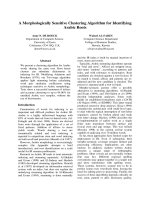
Besides enabling supervision on the cluster sizes, sizeconstrained Shrinkage Clustering is also computationally
advantageous. Figure 2a shows that a larger ω results in
fewer iterations needed for the algorithm to converge, and
the effect reaches a plateau once ω reaches certain sizes
(e.g. ω = 10 in this case). The shrinkage paths (Fig. 2b)
show that it is the reduced number of iterations at the
beginning of a run that speeds up the entire process of
solution finding when ω is large.
In reality, it is rare to find a perfectly binary similarity
matrix similar to what we generated from a known cluster assignment matrix. There is always a certain degree of
noise clouding our observations. To investigate how much
noise the algorithm can tolerate in the data, we add a layer

a

of Gaussian noise over the simulated similarity matrix.
Since Sij ∈ {0, 1}, we create a new similarity matrix SN
containing noise defined by
SijN =

|εij |
1 − |εij |

if Sij = 0
,
if Sij = 1

where εij ∼ N 0, σ 2 . The standard deviation σ is varied from 0 to 0.5, and SN is generated 1000 times by
randomly sampling εij with each σ value. Figure 3a illustrates the changes of the similarity distribution density as
σ increases. When σ = 0 (i.e. no noise), SN is Bernoulli
distributed. As σ becomes larger and larger, the bimodal
shape is flattened by noise. When σ = 0.5, approximately
32% of the similarity relationships are reversed, and hence
observations have been perturbed too much to infer the
underlying cluster structure. The performances of Shrinkage Clustering in these noisy conditions are shown in
Fig. 3b. The algorithm proves to be quite robust against
noise, as the true cluster structure is 100% recovered in all
conditions except for when σ > 0.4.

b

Fig. 2 Performances of Shrinkage Clustering with cluster size constraints. a The average number of iterations spent is plotted with ω taking values of
1 to 5, 10, 15, 20 and 25. b Example shrinkage paths are shown for ω of 1 to 5, 10, 15, 20 and 25 (path of ω = 10 is in overlap with ω = 15)


Hu et al. BMC Bioinformatics (2018) 19:19

Page 6 of 11

a

b

Fig. 3 Robustness of Shrinkage Clustering against noise. a The distribution density of SN is shown with a varying degree of noise, as ε is sampled with
σ from 0 to 0.5. b The probability of successfully recovering the underlying cluster structure is plotted against different noise levels. The true cluster
recovery is defined as the frequency of generating the exact same cluster assignment as the true cluster assignement when clustering the data with

noise generated 1000 times

Case Study: TCGA Dataset

To illustrate the performance of Shrinkage Clustering on
real biological similarity data, we apply the algorithm
to subtyping tumors from the Cancer Genome Atlas
(TCGA) dataset [30]. Derived from the TCGA database,
the dataset includes 293 samples from 3 types of cancers, which are Breast Invasive Carcinoma (BRCA, 207
samples), Glioblastoma Multiforme (GBM, 67 samples)
and Lung Squamous Cell Carcinoma (LUSC, 19 samples).
The data is presented in the form of a similarity matrix,
which integrates information from the gene expression
levels, DNA methylation and copy number aberration.
Since the similarity scores from the TCGA dataset are in
general skewed to 1, we first normalize the data by shifting its median around 0.5 and by bounding values that are
greater than 1 and smaller than 0 to 1 and 0 respectively.
We then perform Shrinkage Clustering to cluster the cancer samples, the result of which is shown in comparison
to the true cancer types (Table 2). We can see that the
algorithm generates three clusters, successfully predicting
the true number of cancer types contained in the data.
The clustering assignments also demonstrate high accuracy, as 98% of samples are correctly clustered with only 5
samples misclassified. In addition, we compared the performance of Shrinkage Clustering to that of five commonly
used clustering algorithms that directly cluster similarity

Table 2 Clustering results of the TCGA dataset, where the
clustering assignments from Shrinkage Clustering are compared
against the three known tumor types
Tumor Type

Cluster 1

Cluster 2

Cluster 3

BRCA

3

204

0

GBM

0

0

67

LUSC

17

2

0

data: Spectral Clustering [31], Hierarchical Clustering [13]
(Ward’s method [32]), PAM [33], AGNES [34], and SymNMF [28]. Since these five methods do not determine the
optimal cluster number, the mean Silhouette [22] width
is used to pick the optimal cluster number from a range
of 2 to 10 clusters. Notably, Shrinkage Clustering is one
of the two algorithms that estimate a three-cluster structure (with AGNES), and its accuracy outperforms the rest
(Table 5).
Experiments on feature-based data
Testing with simulated and standardized data

Since similarity matrices are not always available in
most clustering applications, we now test the performance of Shrinkage Clustering using feature-based data
that does not directly provide the similarity information between objects. To run Shrinkage Clustering, we
first convert the data to a similarity matrix using S =
exp −(D(X)/(βσ ))2 , where [ D(X)]ij is the Euclidean
distance between Xi and Xj , σ is the standard deviation
of D(X), and β = E D(X)2 /σ 2 . The same conversion
method is used for all datasets in the rest of this paper.
As a proof of concept, we first generate a simulated
three-cluster two-dimensional data set by sampling 50
points for each cluster from bivariate normal distributions with a common identity covariance matrix around
centers at (-2, 2), (-2, 2) and (0, 2) respectively. The clustering result from Shrinkage Clustering is shown in Table 3,
where the algorithm successfully determines the existence
of 3 clusters in the data and obtains a clustering solution
with high accuracy.
Next, we test the performance of Shrinkage Clustering
using two real data sets, the Iris [35] and the wine data
[36], both of which are frequently used to test clustering algorithms; and they can be downloaded from the
University of California Irvine (UCI) machine learning

Hu et al. BMC Bioinformatics (2018) 19:19

Page 7 of 11

Table 3 Performances of Shrinkage Clustering on Simulated, Iris
and Wine data, where the clustering assignments are compared
against the three simulated centers, three Iris species and three
wine types respectively
Simulated

Iris

Wine

Center

C1

C2

C3

Species

C1

C2

Type

C1

C2

C3

(-2,2)

0

49

1

setosa

50

0

1

0

59

0

(-2,-2)

0

1

49

versicolor

0

50

2

59

6

0

(2,0)

50

0

0

virginica

0

50

3

0

6

48

repository [37]. The clustering results from Shrinkage
Clustering for both datasets are shown in Table 3, where
the clustering assignments are compared to the true cluster memberships of the Iris and the wine samples respectively. In application to the wine data, Shrinkage Clustering
successfully identifies a correct number of 3 wine types
and produces highly accurate cluster memberships. For
the Iris data, though the algorithm generates two instead
of three clusters, the result is acceptable because the
species versicolor and virginica are known to be hardly
distinguishable given the features collected.
Case study 1: Breast Cancer Wisconsin Diagnostic (BCWD)

The BCWD dataset [38, 39] contains 569 breast cancer
samples (357 benign and 212 malignant) with 30 characteristic features computed from a digitized image of a
fine needle aspirate (FNA) of a breast mass. The dataset
is available on the UCI machine learning repository [37]
and is one of the most popularly tested dataset for clustering and classification. Here, we apply Shrinkage Clustering
to the data and compare its performance against nine

commonly used clustering methods: Spectral Clustering
[31], K-means [14], Hierarchical Clustering [13] (Ward’s
method [32]), PAM [33], DBSCAN [16], Affinity Propagation [40], AGNES [34], clusterdp [41], SymNMF [28].
Since K-means, Spectral Clustering, Hierarchical Clustering, PAM, AGNES and SymNMF do not inherently determine the optimal cluster number and require the cluster
number as an input, we first run these algorithms with
cluster numbers from 2 to 10, and then use the mean Silhouette width as the criterion to select the optimal cluster
number. For algorithms that internally select the optimal cluster number (i.e. DBSCAN, Affinity Propagation
and clusterdp), we tune the parameters to generate clustering solutions with cluster numbers similar to the true
cluster numbers so that the accuracy comparison is less
biased. The parameter values for each algorithm are specified in Table 4. For DBSCAN, the clustering memberships
of non-noise samples are used for assessing accuracy.
The accuracy of all clustering solutions is evaluated using
four metrics: Normalized Mutual Information (NMI) [42],
Rand Index [42], F1 score [42], and the optimal cluster
number (K).

Table 4 Parameter values of DBSCAN, Affinity Propagation and
clusterdp
Algorithm

DBSCAN

Affinity propagation

clusterdp

Parameter

minPts

eps

p

q

rho

delta

BCWD

31

3000

NA

0

20

3000

Dyrskjot-2003

2

23000

NA

0.07

3

20000

Nutt-2003-v1

2

11000

NA

0.12

1.5

3000

Nutt-2003-v3

1

8000

NA

0.1

1

7000

AIBT

5

400

NA

0

2.5

240

The performance results (Table 5) show that Shrinkage Clustering correctly predicts a 2 cluster structure
from the data and generates the clustering assignments
with high accuracy. When comparing the cluster assignments against the true cluster memberships, we can see
that Shrinkage Clustering is among the top three best
performers across all accuracy metrics.
Case study 2: Benchmarking gene expression data for
cancer subtyping

Next, we test the performance of Shrinkage Clustering as
well as the nine commonly used algorithms in application

to identifying cancer subtypes using three benchmarking datasets from de Souto et al. [43]: Dyrskjot-2003 [44],
Nutt-2003-v1 [45] and Nutt-2003-v3 [45]. Dyrskjot-2003
contains the expression levels of 1203 genes in 40 wellcharacterized bladder tumor biopsy samples from three
subclasses of bladder carcinoma: T2+ (9 samples), Ta (20
samples), and T1 (11 samples). Nutt-2003-v1 contains
the expression levels of 1377 genes in 50 gliomas from
four subclasses: classic gliobalstomas (14 samples), classic anaplastic oligodendrogliomas (7 samples), nonclassic
glioblastomas (14 samples), and nonclassic anaplastic
oligodendrogliomas (15 samples). Nutt-2003-v3 is a subset of Nutt-2003-v1, containing 7 samples of classic
anaplastic oligodendrogliomas and 15 samples of nonclassic anaplastic oligodendrogliomas with the expression of
1152 genes. All three data sets are small in sample sizes
and high in dimensions, which is often the case in clinical
research. The performance of all ten algorithms is compared using the same metrics as in the previous case study,
and the result is shown in Table 5. Though there is no clear
winning algorithm across all data sets, Shrinkage Clustering is among the top three performers in all cases, along
with other top performing algorithms such as SymNMF,
K-means and DBSCAN. Since the clustering results from
DBSCAN are compared to the true cluster assignments
excluding the noise samples, the accuracy of DBSCAN
may be slightly overestimated.
Case Study 3: Allen Institute Brain Tissue (AIBT)

The AIBT dataset [46] contains RNA sequencing data
of 377 samples from four types of brain tissues, i.e. 99


Hu et al. BMC Bioinformatics (2018) 19:19

Page 8 of 11

Table 5 Performance comparison of ten algorithms on six biological data sets, i.e. TCGA, BCWD, Dyrskjot-2003, Nutt-2003-v1,
Nutt-2003-v3 and AIBT
Data

TCGA

BCWD

Dyrskjot-2003

Nutt-2003-v1

Nutt-2003-v3

AIBT

Metric

Shrinkage

Spectral

K-means

Hierarchical

PAM

DBSCAN

Affinity

AGNES

Clusterdp

SymNMF

NMI

0.91

0.77

NA

0.83

0.76

NA

NA

0.82

NA

0.78

Rand

0.97

0.91

NA

0.91

0.77

NA

NA

0.90

NA

0.94

F1

0.98

0.92

NA

0.92

0.80

NA

NA

0.92

NA

0.95

K (3)

3

2

NA

2

2

NA

NA

3

NA

2

NMI

0.50

0.29

0.46

0.09

0.50

0.20

0.45

0.09

0.20

0.56

Rand

0.77

0.68

0.75

0.55

0.77

0.64

0.76

0.55

0.53

0.83

F1

0.80

0.69

0.79

0.69

0.80

0.75

0.79

0.69

0.59

0.85

K (2)

2

2

2

2

2

2

3

2

2

2

NMI

0.45

0.07

0.51

0.12

0.56

0.30

0.42

0.12

0.07

0.58

Rand

0.78

0.55

0.76

0.42

0.77

0.55

0.72

0.42

0.50

0.83

F1

0.70

0.36

0.71

0.54

0.66

0.60

0.66

0.54

0.43

0.75

K (3)

3

3

3

3

3

3

3

3

2

3

NMI

0.56

0.45

0.47

0.28

0.34

0.61

0.41

0.11

0.17

0.49

Rand

0.72

0.73

0.72

0.52

0.68

0.65

0.73

0.35

0.64

0.72

F1

0.58

0.51

0.51

0.43

0.41

0.62

0.44

0.38

0.34

0.55

K (4)

4

4

4

4

4

4

5

4

4

4

NMI

1.00

0.20

0.75

0.13

0.33

0.13

0.13

0.13

0.29

0.76

Rand

1.00

0.58

0.91

0.58

0.58

0.58

0.58

0.58

0.55

0.91

F1

1.00

0.59

0.92

0.71

0.60

0.71

0.71

0.71

0.57

0.91

K (2)

2

2

2

2

2

2

3

2

2

2

NMI

0.56

0.20

0.58

0.17

0.54

0.56

0.53

0.02

0.55

0.55

Rand

0.79

0.68

0.80

0.37

0.78

0.65

0.76

0.26

0.69

0.79

F1

0.61

0.39

0.62

0.40

0.59

0.59

0.51

0.40

0.57

0.61

K (4)

4

4

4

4

4

4

5

4

3

4

Clustering accuracy is assessed via metrics including NMI (Normalized Mutual Information), Rand Index, F1 score and K (the optimal cluster number). The top three
performers in each case are highlighted in bold

samples of temporal cortex, 91 samples of parietal cortex, 93 samples of cortical white matter, and 94 samples

hippocampus isolated by macro-dissection. For each sample, the expression levels of 50282 genes are included
as features, and each feature is normalized to have a
mean of 0 and a standard deviation of 1 prior to testing. In contrast to the previous case study, the AIBT
data is much larger in size with significantly more features being measured. Therefore, this would be a great
example to test both the accuracy and the speed of clustering algorithms in face of greater data sizes and higher
dimensions.
Similar to the previous case studies, we apply Shrinkage Clustering and the nine commonly used clustering
algorithms to the data, and use mean Silhouette width
to select the optimal cluster number for algorithms that
do not inherently determine the cluster number. The

performances of all ten algorithms measured across the
four accuracy metrics (i.e. NMI, Rand, F1, K) are shown
in Table 5. We can see that Shrinkage Clustering is the
second best performer among all ten algorithms in terms
of clustering quality, with comparable accuracy to the top
performer (K-means).
Next, we record and compare the speed of the ten
algorithms for clustering the data. The speed comparison results, shown in Fig. 4, demonstrate the unparalleled
speed of Shrinkage Clustering compared to the rest of
the algorithms. Compared to algorithms that automatically select optimal number of clsuters (DBSCAN, Affinity Propagation and Clusterdp), Shrinkage Clustering is
two times faster in speed; compared to algorithms that
are coupled with external cluster validation algorithms
for cluster number selection, Shrinkage Clustering is at
least 14 times faster. In particular, the same data that


Hu et al. BMC Bioinformatics (2018) 19:19

Page 9 of 11

Fig. 4 Speed comparison using the AIBT data. The computation time of Shrinkage Clustering is recorded and compared against other commonly
used clustering algorithms

takes Shrinkage Clustering only 73 s to cluster can take
Spectral clustering more than 20 h.

Discussion
From the biological case studies, we showed that
Shrinkage Clustering is computationally advantageous in
speed with comparable clustering accuracy to top performing clustering algorithms and higher clustering accuracy than algorithms that internally select cluster numbers.
The advantage in speed mainly comes from the fact that
Shrinkage Clustering integrates the clustering of the data
and the determination of the optimal cluster number into
one seamless process, so the algorithm only needs to run
once in order to complete the clustering task. In contrast, algorithms like K-means, PAM, Spectral Clustering,
AGNES and SymNMF perform clustering on a single cluster number basis, therefore they need to be repeatedly
run for all cluster numbers of interest before a clustering
evaluation method can be applied. Notably, the clustering
evaluation method Silhouette that we used in this experiment does not perform any repetitive clustering validation
and therefore is a much faster method compared to other
commonly used methods that require repetitive validation
[27]. This means that Shrinkage Clustering would have an
even greater advantage in computation speed compared
to the methods tested in this paper if we use a cluster evaluation method that has a repetitive nature (e.g. Consensus
Clustering, Gap Statistics, Stability Selection).
One prominent feature of Shrinkage Clustering is its
flexibility to add the constraint of minimum cluster sizes.
The size constraints can help prevent generating empty
or tiny clusters (which are often observed in Hierarchical

Clustering and sometimes in K-means applications), and
can produce clusters of sufficiently large sample sizes as
required by the user. This is particularly useful when we
need to perform subsequent statistical analyses based on

the clustering solution, since clusters of too small a size
can make a statistical testing infeasible. For example, one
application of cluster analysis in clinical studies is identifying subpopulations of cancer patients based on their
gene expression levels, which is usually followed with a
survival analysis to determine the prognostic value of the
gene expression patterns. In this case, clusters that contain too few patients can hardly generate any significant
or meaningful patient outcome comparison. In addition,
it is difficult to take actions based on tiny patient clusters
(e.g. in the context of designing clinical trials), because
these clusters are hard to validate. Since adding minimum
size constraints is essentially merging tiny clusters into
larger ones and might result in less homogeneous clusters,
this approach is unfavorable if the researcher wishes to
identify the outliers in the data or to obtain more homogeneous clusters. In these scenarios, we would recommend
using the base algorithm without adding the minimum
size constraint.
Despite its superior speed and high accuracy, Shrinkage
Clustering has a couple of limitations. First, the automatic convergence to an optimal cluster number is a
double-edged sword. This feature helps to determine the
optimal cluster number and speeds up the clustering process dramatically, however it can be unfavorable when the
researcher has a desired cluster number in mind that is
different from the cluster number identified by the algorithm. Second, the algorithm is based on the assumption
of hard clustering, therefore it currently does not provide probabilistic frameworks as those offered by soft
clustering. In addition, due to the similarity between symNMF and K-means, the algorithm likely prefers spherical clusters if the similarity matrix is derived from
Euclidean distances. Interesting future research directions

include exploring and extending the capability of Shrinkage Clustering to identify oddly-shaped clusters, to deal


Hu et al. BMC Bioinformatics (2018) 19:19

with missing data or incomplete similarity matrices, as
well as to handle semi-supervised clustering tasks with
must-link and cannot-link constraints.

Page 10 of 11

6.

7.

Conclusions
In summary, we developed a new NMF-based clustering
method, Shrinkage Clustering, which shrinks the number
of clusters to an optimum while simultaneously optimizing the cluster memberships. The algorithm performed
with high accuracy on both simulated and actual data,
exhibited excellent robustness to noise, and demonstrated
superior speeds compared to some of the commonly used
algorithms. The base algorithm has also been extended
to accommodate requirements on minimum cluster sizes,
which can be particularly beneficial to clinical studies and
the general biomedical community.
Acknowledgements
Not applicable.
Funding
This research was funded in part by NSF CAREER 1150645 and NIH R01

GM106027 grants to A.A.Q., and a HHMI Med-into-Grad fellowship to C.W. Hu.
Availability of data and materials
The datasets used in this study are publicly available (see references in the text
where each dataset is first introduced).
Authors’ contributions
Method conception and development: CWH; method testing and manuscript
writing: CWH, HL, AAQ; study supervision: AAQ. All authors read and approved
the final manuscript.
Ethics approval and consent to participate
Not applicable.

8.

9.

10.

11.
12.
13.
14.

15.
16.

17.
18.
19.
20.

Consent for publication
Not applicable.
Competing interests
The authors declare that they have no competing interests.

Publisher’s Note
Springer Nature remains neutral with regard to jurisdictional claims in
published maps and institutional affiliations.

21.

22.
23.

Received: 20 June 2017 Accepted: 10 January 2018
24.
References
1. Sørlie T, Tibshirani R, Parker J, Hastie T, Marron J, Nobel A, et al.
Repeated observation of breast tumor subtypes in independent gene
expression data sets. Proc Natl Acad Sci. 2003;100(14):8418–23.
2. Wirapati P, Sotiriou C, Kunkel S, Farmer P, Pradervand S, Haibe-Kains B,
et al. Meta-analysis of gene expression profiles in breast cancer: toward a
unified understanding of breast cancer subtyping and prognosis
signatures. Breast Cancer Res. 2008;10(4):R65.
3. Rouzier R, Perou CM, Symmans WF, Ibrahim N, Cristofanilli M,
Anderson K, et al. Breast cancer molecular subtypes respond differently to
preoperative chemotherapy. Clin Cancer Res. 2005;11(16):5678–85.
4. Abascal F, Valencia A. Clustering of proximal sequence space for the
identification of protein families. Bioinformatics. 2002;18(7):908–21.
5. Stam MR, Danchin EG, Rancurel C, Coutinho PM, Henrissat B. Dividing

the large glycoside hydrolase family 13 into subfamilies: towards
improved functional annotations of α-amylase-related proteins. Protein
Eng Des Sel. 2006;19(12):555–62.

25.

26.
27.

28.

29.
30.

de Lima EB, Júnior WM, de Melo-Minardi RC. Isofunctional Protein
Subfamily Detection Using Data Integration and Spectral Clustering. PLoS
Comput Biol. 2016;12(6):e1005001.
Chen X, Velliste M, Weinstein S, Jarvik JW, Murphy RF. Location
proteomics—Building subcellular location tree from high resolution 3D
fluorescence microcope images of randomly-tagged proteins.
Manipulation and Analysis of Biomolecules, Cells, and Tissues,
Proceedings of SPIE 4962; 2003, pp. 298–306.
Slater JH, Culver JC, Long BL, Hu CW, Hu J, Birk TF, et al. Recapitulation
and modulation of the cellular architecture of a user-chosen cell of
interest using cell-derived, biomimetic patterning. ACS nano. 2015;9(6):
6128–38.
Haldar P, Pavord ID, Shaw DE, Berry MA, Thomas M, Brightling CE, et al.
Cluster analysis and clinical asthma phenotypes. Am J Respir Crit Care
Med. 2008;178(3):218–24.
Moore WC, Meyers DA, Wenzel SE, Teague WG, Li H, Li X, et al.

Identification of asthma phenotypes using cluster analysis in the Severe
Asthma Research Program. Am J Respir Crit Care Med. 2010;181(4):315–23.
Jain AK, Murty MN, Flynn PJ. Data clustering: a review. ACM Comput Surv
(CSUR). 1999;31(3):264–323.
Wiwie C, Baumbach J, Röttger R. Comparing the performance of
biomedical clustering methods. Nat Med. 2015;12(11):1033–8.
Johnson SC. Hierarchical clustering schemes. Psychometrika. 1967;32(3):
241–54.
MacQueen J, et al. Some methods for classification and analysis of
multivariate observations. In: Proceedings of the fifth Berkeley
symposium on mathematical statistics and probability, vol. 1, No. 14.
California: University of California Press; 1967. p. 281–97.
Lloyd S. Least squares quantization in PCM. Inf Theory IEEE Trans.
1982;28(2):129–37.
Ester M, Kriegel HP, Sander J, Xu X. A density-based algorithm for
discovering clusters in large spatial databases with noise. In: KDD. vol. 96,
No. 34. Portland; 1996. p. 226–31.
McLachlan GJ, Basford KE. Mixture models: inference and applications to
clustering. New York: Marcel Dekker; 1988.
Shi J, Malik J. Normalized cuts and image segmentation. Pattern Anal
Mach Intell IEEE Trans. 2000;22(8):888–905.
Li T, Ding CH. Data Clustering: Algorithms and Applications. Boca Raton:
CRC Press; 2013, pp. 149–76.
Ding C, He X, Simon HD. On the equivalence of nonnegative matrix
factorization and spectral clustering. In: Proceedings of the 2005 SIAM
International Conference on Data Mining. Philadelphia: SIAM; 2005.
p. 606–10.
Brunet JP, Tamayo P, Golub TR, Mesirov JP. Metagenes and molecular
pattern discovery using matrix factorization. Proc Natl Acad Sci.
2004;101(12):4164–9.

Rousseeuw PJ. Silhouettes: a graphical aid to the interpretation and
validation of cluster analysis. J Comput Appl Math. 1987;20:53–65.
Pelleg D, Moore AW, et al. X-means: Extending K-means with Efficient
Estimation of the Number of Clusters. In: ICML ’00 Proceedings of the
Seventeenth International Conference on Machine Learning. San
Francisco: Morgan Kaufmann Publishers Inc.; 2000. p. 727–734.
Tibshirani R, Walther G, Hastie T. Estimating the number of clusters in a
data set via the gap statistic. J R Stat Soc Ser B Stat Methodol. 2001;63(2):
411–23.
Monti S, Tamayo P, Mesirov J, Golub T. Consensus clustering: a
resampling-based method for class discovery and visualization of gene
expression microarray data. Mach Learn. 2003;52(1-2):91–118.
Lange T, Roth V, Braun ML, Buhmann JM. Stability-based validation of
clustering solutions. Neural Comput. 2004;16(6):1299–323.
Hu CW, Kornblau SM, Slater JH, Qutub AA. Progeny Clustering: A
Method to Identify Biological Phenotypes. Sci Rep. 2015;5(12894):5.
/>Kuang D, Ding C, Park H. Symmetric nonnegative matrix factorization for
graph clustering. In: Proceedings of the 2012 SIAM international
conference on data mining. Philadelphia: SIAM; 2012. p. 106–17.
Bradley P, Bennett K, Demiriz A. Constrained k-means clustering.
Redmond: Microsoft Research; 2000, pp. 1–8.
Speicher N, Lengauer T. Towards the identification of cancer subtypes by
integrative clustering of molecular data. Saarbrücken: Universität des
Saarlandes; 2012.


Hu et al. BMC Bioinformatics (2018) 19:19

Page 11 of 11

31. Zeileis A, Hornik K, Smola A, Karatzoglou A. kernlab-an S4 package for
kernel methods in R. J Stat Softw. 2004;11(9):1–20.
32. Ward Jr JH. Hierarchical grouping to optimize an objective function. J Am
Stat Assoc. 1963;58(301):236–44.
33. Maechler M, Rousseeuw P, Struyf A, Hubert M, Hornik K. Cluster: cluster
analysis basics and extensions. R Package Version. 2012;1(2):56.
34. Kaufman L, Rousseeuw PJ. Finding groups in data: an introduction to
cluster analysis, vol. 344. Hoboken: John Wiley & Sons; 2009.
35. Fisher RA. The use of multiple measurements in taxonomic problems.
Ann Eugenics. 1936;7(2):179–88.
36. Aeberhard S, Coomans D, De Vel O. Comparison of classifiers in high
dimensional settings. Dept Math Statist, James Cook Univ, North
Queensland, Australia. Tech Rep. 1992;92-02.
37. Bache K, Lichman M. UCI Machine Learning Repository: University of
California, Irvine, School of Information and Computer Sciences; 2013.
/>38. Street WN, Wolberg WH, Mangasarian OL. Nuclear feature extraction for
breast tumor diagnosis. In: IS&T/SPIE’s Symposium on Electronic Imaging:
Science and Technology. San Jose: International Society for Optics and
Photonics; 1993. p. 861–70.
39. Mangasarian OL, Street WN, Wolberg WH. Breast cancer diagnosis and
prognosis via linear programming. Oper Res. 1995;43(4):570–7.
40. Frey BJ, Dueck D. Clustering by passing messages between data points.
Science. 2007;315(5814):972–6.
41. Rodriguez A, Laio A. Clustering by fast search and find of density peaks.
Science. 2014;344(6191):1492–6.
42. Manning CD, Raghavan P, Schütze H, et al. Introduction to information
retrieval, vol. 1. Cambridge: Cambridge university press; 2008.
43. de Souto MC, Costa IG, de Araujo DS, Ludermir TB, Schliep A. Clustering
cancer gene expression data: a comparative study. BMC Bioinformatics.
2008;9(1):497.

44. Dyrskjøt L, Thykjaer T, Kruhøffer M, Jensen JL, Marcussen N,
Hamilton-Dutoit S, et al. Identifying distinct classes of bladder carcinoma
using microarrays. Nat Genet. 2003;33(1):90.
45. Nutt CL, Mani D, Betensky RA, Tamayo P, Cairncross JG, Ladd C, et al.
Gene expression-based classification of malignant gliomas correlates
better with survival than histological classification. Cancer Res. 2003;63(7):
1602–7.
46. Montine JT, Sonnen AJ, Montine SK, Crane KP, Larson BE. Adult Changes
in Thought study: dementia is an individually varying convergent
syndrome with prevalent clinically silent diseases that may be modified by
some commonly used therapeutics. Curr Alzheim Res. 2012;9(6):718–23.

Submit your next manuscript to BioMed Central
and we will help you at every step:
• We accept pre-submission inquiries
• Our selector tool helps you to find the most relevant journal
• We provide round the clock customer support
• Convenient online submission
• Thorough peer review
• Inclusion in PubMed and all major indexing services
• Maximum visibility for your research
Submit your manuscript at
www.biomedcentral.com/submit