SPRINT: Ultrafast protein-protein interaction prediction of the entire human interactome
Bạn đang xem bản rút gọn của tài liệu. Xem và tải ngay bản đầy đủ của tài liệu tại đây (1.4 MB, 11 trang )
Li and Ilie BMC Bioinformatics (2017) 18:485
DOI 10.1186/s12859-017-1871-x
SOFTWAR E
Open Access
SPRINT: ultrafast protein-protein
interaction prediction of the entire human
interactome
Yiwei Li and Lucian Ilie*
Abstract
Background: Proteins perform their functions usually by interacting with other proteins. Predicting which proteins
interact is a fundamental problem. Experimental methods are slow, expensive, and have a high rate of error. Many
computational methods have been proposed among which sequence-based ones are very promising. However, so far
no such method is able to predict effectively the entire human interactome: they require too much time or memory.
Results: We present SPRINT (Scoring PRotein INTeractions), a new sequence-based algorithm and tool for predicting
protein-protein interactions. We comprehensively compare SPRINT with state-of-the-art programs on seven most
reliable human PPI datasets and show that it is more accurate while running orders of magnitude faster and using
very little memory.
Conclusion: SPRINT is the only sequence-based program that can effectively predict the entire human interactome:
it requires between 15 and 100 min, depending on the dataset. Our goal is to transform the very challenging problem
of predicting the entire human interactome into a routine task.
Availability: The source code of SPRINT is freely available from and the
datasets and predicted PPIs from www.csd.uwo.ca/faculty/ilie/SPRINT/.
Keywords: Protein-protein interaction (PPI), PPI prediction, Human interactome
Background
Protein-protein interactions (PPI) play a key role in many
cellular processes since proteins usually perform their
functions by interacting with other proteins. Genomewide identification of PPIs is of fundamental importance
in understanding the cell regulatory mechanisms [1] and
PPI identification is one of the major objectives of systems
biology. Various experimental techniques for identifying
PPIs have been developed, most notably high throughput
procedures such as two-hybrid assay and affinity systems
[2]. Such methods are slow and expensive and have a
high rate of error. A variety of computational methods
have been designed to help predicting PPIs, employing sequence homology, gene co-expression, phylogenetic
profiles, etc. [3–5].
*Correspondence:
Department of Computer Science, The University of Western Ontario, N6A 5B7
London, Ontario, Canada
Sequence-based approaches [6–17] are faster and
cheaper and can be used in addition to other methods,
to improve their performance. Several top methods were
evaluated by Park [18]. Park and Marcotte [19] made the
crucial observation that the datasets previously used for
evaluation were biased due to the frequent occurrence
of protein pairs common to testing and training data.
They have shown that the prediction of the algorithms
on the testing protein pairs is improved when the protein
sequences are seen in training. To avoid this bias, they
have built datasets of three levels of difficulty such that the
predictive performance on these datasets generalizes to
the population level. The performance of the top methods
tested by Park [18] on the unbiased datasets of [19] was
significantly lower than previously published, thus raising
the bar higher for sequence-based methods.
We introduce a new sequence-based PPI prediction
method, SPRINT (Scoring PRotein INTeractions), that is
more accurate than the current state-of-the-art methods
© The Author(s). 2017 Open Access This article is distributed under the terms of the Creative Commons Attribution 4.0
International License ( which permits unrestricted use, distribution, and
reproduction in any medium, provided you give appropriate credit to the original author(s) and the source, provide a link to the
Creative Commons license, and indicate if changes were made. The Creative Commons Public Domain Dedication waiver
( applies to the data made available in this article, unless otherwise stated.
Li and Ilie BMC Bioinformatics (2017) 18:485
as well as orders of magnitude faster. The SPRINT algorithm relies on the same basic hypothesis that underlies
most sequence-based approaches: a pair of proteins that
are pairwise similar with a pair of interacting proteins
has a higher chance to interact. However, the way this
idea is used is very different. Similar regions are identified using an effective multiple spaced-seed approach
and then processed to eliminate elements that occur too
often to be involved in interactions. Finally, a score is computed for each protein pair such that high scores indicate
increased probability of interactions. Details are given in
the “Methods” section.
We compared SPRINT with the top programs considered by Park [18] and Park and Marcotte [19] as well as the
new method of Ding et al. [20]. The closest competitors
are the machine learning-based programs of Ding et al.
[20] and Martin et al. [6], and PIPE2 [7, 21], which does
not use machine learning. All comparisons are done using
human datasets.
To comprehensively compare the performance, we use
multiple datasets, built according to the procedure of Park
and Marcotte [19] from six of the most reliable human
PPI databases: Biogrid, HPRD, InnateDB (experimentally
validated and manually curated PPIs), IntAct, and MINT.
SPRINT provides the best predictions overall, especially
for the more difficult C2 and C3 types.
Then, we use the entire human interactome to compare the speed. The comparisons of [18] and [19] used
fairly small datasets for comparison. In reality, these programs are meant to be used on entire proteomes and
interactomes, where all protein sequences and known
interactions are involved. SPRINT is several orders of
magnitude faster. It takes between 15 and 100 min
on a 12-core machine while the closest competitor,
Ding’s program, requires weeks and Martin’s and PIPE2
require years. Moreover, Ding’s program is unable to
run the larger datasets as its memory requirements are
very high.
The source code of SPRINT is freely available.
Results
We compare in this section SPRINT with several stateof-the-art sequence-based programs for PPI prediction
on the most important human PPI datasets available. We
focus on accurate prediction of the entire human interactome and therefore we have been using only human
datasets. We start with a discussion concerning the
datasets employed, as the way they are constructed can
significantly impact the performance of the predicting
programs.
Park and Marcotte’s evaluation scheme
Park and Marcotte [19] noticed that all methods have significantly higher performance for the protein pairs in the
Page 2 of 11
testing data whose sequences appear also in the training
data. Three cases are possible, depending on whether both
proteins in the test data appear in training (C1), only one
appears (C2), or none (C3). They show that essentially
all datasets previously used for cross validation are very
close to the C1 type, whereas in the HIPPIE meta-database
of human PPIs [22] the C1-type human protein pairs
accounts for only 19.2% of these cases, whereas C2-type
and C3-type pairs make up 49.2% and 31.6%, respectively. Therefore, testing performed on C1-type data is
not expected to generalize well to the full population. The
authors proceeded to designing three separate human PPI
datasets that follow the C1, C2, and C3-type rules.
Datasets
We first describe the procedure of Park and Marcotte [19]
in detail. The protein sequences are from UniProt [23].
The interactions were downloaded from the protein interaction network analysis platform [24] that integrates data
from six public PPI databases: IntAct [25], MINT [26],
BioGRID [27], DIP [28], HPRD [29] and MIPS MPact [30].
The datasets were processed by [19] as follows. Proteins in
each data set were clustered using CD-HIT2 [31] such that
they shared sequence identity less than 40%. Proteins with
less than 50 amino acids as well as homo-dimeric interactions were removed. Negative PPI data were generated
by randomly sampling protein pairs that are not known to
interact. See [19] for more details.
The total number of proteins used is 20,117, involving
24,718 PPIs. The training and testing datasets are divided
into forty splits (from the file human_random.tar.gz), each
consisting of one training file and three testing files, one
for each type C1, C2, C3. Therefore, each C1, C2, or
C3 curve produced is the average of forty curves. In
addition, they tested also 40-fold cross validation on the
entire PPI set. In reality, the ratio between interacting and
noninteracting protein pairs is believed to be 1:100 or
lower. However, this would make it very slow or impossible to run some of the algorithms. Therefore, Park and
Marcotte decided to use ratio 1:1.
We have used Park and Marcotte’s procedure to design
similar testing datasets using six other human PPI
databases. Among the most widely known human PPI
databases we have chosen six that appear to be the most
widely used: Biogrid, HPRD, InnateDB (experimentally
validated and manually curated PPIs), IntAct, and MINT.
We have used 20,160 human protein sequences downloaded from UniProt. The protein sequences and interactions were downloaded in Oct. 2016. We perform four
tests for each program on each dataset: 10 fold crossvalidation using all PPIs and C1, C2, and C3 tests, the
datasets for which are built as explained above, with the
ratio between training and testing pairs of 10:1. The details
of all datasets are given in Table 1.
Li and Ilie BMC Bioinformatics (2017) 18:485
Page 3 of 11
Competing methods
We have compared SPRINT with the four methods considered by [19]. Three of those use machine learning: [6],
[8], and [9], whereas the fourth does not: PIPE [7]. Since
the first three methods do not have names, we use the
first author’s name to identify them: Martin [6], Shen
[8], and Guo [9]. Note that we have tested the improved
PIPE2 [21], the same version that was tested by Park and
Marcotte.
Many programs have been proposed for PPI prediction,
however, very few are available. We have obtained the
source code for two programs: the PPI-PK method of [10]
and the program of Ding et al. [20]. The PPI-PK method
was too slow on our system to be tested. We managed to
run the program of Ding et al. [20] on all datasets. After
eliminating the programs of Shen et al. [8] and Guo et al.
[9] as placing last on the first datasets, comparison on all
subsequent tests were performed against Martin, PIPE2,
and Ding.
Note that PIPE2 and SPRINT do not require negative
training data as they do not use machine learning algorithms. All the other programs require both positive and
negative training sets. Note also that Ding’s program uses
also additional information concerning electrostatic and
hydrophobic properties of amino acids.
Performance comparison
Park and Marcotte datasets
We present first the comparison of all five methods considered on the datasets of Park and Marcotte in Fig. 1. The
receiver operating characteristic (ROC) and precisionrecall (PR) curves for the four tests, CV, C1, C2, and C3,
are presented.
The prediction performance on CV and C1 is very similar. The performance decreases from C1 to C2 and again
to C3, both for ROC and PR curves. This is expected
due to the way the datasets are constructed. The ROC
curves do not distinguish very well between the prediction performance of the five methods. The difference is
more clear in the PR curves. The SPRINT curve is almost
always on top, especially at the beginning of the curve,
where it matters the most for prediction. Ding’s and Martin’s are very close for CV and C1 datasets, followed by
PIPE2. For C2 and C3 tests, the performance of Ding’s and
Martin’s programs deteriorates and PIPE2 advances in
second position.
Seven human PPI databases
For a comprehensive comparison, we have compared the
top four programs on six datasets, computed as mentioned above from six databases: Biogrid, HPRD Release 9,
InnateDB (experimentally validated and manually curated
PPIs), IntAct, and MINT. Since the prediction on the CV
datasets is similar with C1, we use only C1, C2 and C3
datasets.
For the purpose of predicting new PPIs, the behaviour
at high specificity is important. We therefore compare
the sensitivity, precision and F1 -score for several high
specificity values. The table with all values is given in
the Additional file 1. We present here in Table 2 the
average values for each dataset type (C1, C2, and C3)
over all datasets for each specificity value. At the bottom of the table we give also the average over all three
dataset types. The performance of SPRINT with respect
to all three measures, sensitivity, precision, and F1 -score
is the highest. Only Ding comes close for C1 datasets. the
overall average of SPRINT is much higher than Ding’s.
PIPE2 comes third and Martin last. The performance
of PIPE2 decreases much less from C1 to C3 compared with Ding’s. It should be noted that a weighted
overall average, where the contribution of each dataset
type C1,2,3 is proportional with its share of the general population, would place PIPE2 slightly ahead of
Ding.
The area under the ROC and PR curves is given in
Table 3 for all seven datasets, including the C1-, C2-,
and C3-average, as well as the overall average across
types. Ding is the winner for the C1 tests and SPRINT
Table 1 The datasets used for comparing PPI prediction methods
Dataset
PPIs
Website
All
Park and Marcotte
Biogrid
HPRD release 9
InnateDB experim. validated
InnateDB manually curated
Training
Testing
24,718
14,186
1250
215,029
100,000
10,000
www.marcottelab.org/differentialGeneralization
34,044
10,000
1000
www.hprd.org
165,655
65,000
6500
www.innatedb.com
www.innatedb.com
9913
3600
360
IntAct
111,744
52,500
5250
www.ebi.ac.uk/intact
MINT
16,914
7000
700
mint.bio.uniroma2.it
The second column contains the total number of PPIs, while the third the fourth columns give the number of PPIs used for training and testing, respectively, in the C1, C2,
and C3 tests
Li and Ilie BMC Bioinformatics (2017) 18:485
Page 4 of 11
Table 2 Performance comparison at high specificity
Sensitivity, precision, and F1 -score averages for seven datasets are given for each dataset type C1, C2 and C3, as well as overall averages across types. Darker colours represent
better results. The best results are in bold
is the winner for the C2 and C3 tests. In the overall average, SPRINT comes on top. Martin is third and
PIPE2 last.
All ROC and PR curves are included in the Additional
file 2.
0.8
0.2
0.6
0.8
1.0
0.4
0.6
0.8
1.0
1.0
0.8
0.4
0.2
0.4
0.6
0.8
1.0
0.4
0.6
0.8
1.0
0.4
0.6
0.8
1.0
1.0
Martin
Shen
Guo
PIPE
Ding
SPRINT
0.8
0.7
Martin
Shen
Guo
PIPE
Ding
SPRINT
0.5
0.2
0.2
0.9
0.9
0.8
0.7
0.6
0.0
0.0
Park and Marcotte (C3, PR)
1.0
1.0
0.8
0.7
0.6
Martin
Shen
Guo
PIPE
Ding
SPRINT
0.5
0.2
0.2
Park and Marcotte (C2, PR)
0.9
0.9
0.8
0.7
0.6
0.5
Martin
Shen
Guo
PIPE
Ding
SPRINT
0.0
0.0
Park and Marcotte (C1, PR)
1.0
Park and Marcotte (CV, PR)
0.4
Martin
Shen
Guo
PIPE
Ding
SPRINT
0.0
0.2
0.0
0.0
0.0
1.0
Martin
Shen
Guo
PIPE
Ding
SPRINT
0.6
0.6
Martin
Shen
Guo
PIPE
Ding
SPRINT
0.0
0.5
0.4
0.6
0.8
0.6
0.4
0.6
0.4
0.2
0.2
Park and Marcotte (C3, ROC)
1.0
1.0
Park and Marcotte (C2, ROC)
0.8
0.8
0.6
0.4
0.2
0.0
Martin
Shen
Guo
PIPE
Ding
SPRINT
0.0
The goal of all PPI prediction methods is to predict new
interactions from existing reliable ones. That means, in
practice we input all known interactions – the entire interactome of an organism – and predict new ones. Of the
Park and Marcotte (C1, ROC)
1.0
Park and Marcotte (CV, ROC)
Predicting the entire human interactome
0.2
0.4
0.6
0.8
1.0
0.0
0.2
0.4
0.6
0.8
Fig. 1 Performance comparison on Park and Marcotte datasets: ROC and PR curves. The ROC curves (top row) and PR curves (bottom row) for CV,
C1, C2, and C3 tests, from left to right
1.0
Li and Ilie BMC Bioinformatics (2017) 18:485
Page 5 of 11
Table 3 Area under curves
AUROC and AUPR curves are given for seven datasets and three types, C1, C2, C3, for each, as well as averages for each type and overall average across types. Darker colours
represent better results. The best results are in bold
newly predicted interactions, only those that are the most
likely to be true interactions are kept.
For predicting the entire interactome, we need to predict the probability of interaction between any two proteins. For N proteins, that means we need to consider
(N 2 + N)/2 protein pairs. For our 20,160 proteins, that
is about 203 million potential interactions. For example,
predicting one pair per second results in over six years of
computation time.
We have tested the four programs, Martin’s, PIPE2,
Ding’s, and SPRINT, on the entire human interactome,
considering as given PPIs each of the six datasets in
Table 1. The tests were performed on a DELL PowerEdge
R620 computer with 12 cores Intel Xeon at 2.0 GHz and
256 GB of RAM, running Linux Red Hat, CentOS 6.3.
The time and memory values are shown in Table 4 for
all three stages: preprocessing, training, and predicting.
For each dataset, training is performed on all PPIs in that
dataset and then predictions are made for all 203 million
protein pairs.
Note that PIPE2 and SPRINT do not require any training. Also, preprocessing is performed only once for all
protein sequences. As long as no protein sequences are
added, no preprocessing needs to be done. For SPRINT,
we provide all necessary similarities for all reviewed
human proteins in UniProt. If new protein sequences
are added, the program has an option (“-add”) that
is able to compute only the new similarities, which is
very fast.
Therefore, the comparison is between predicting time
of PIPE2 and SPRINT and training plus predicting time of
Martin and Ding. PIPE2 and Martin are very slow and the
predicting times are estimated by running the programs
for 100 h and then estimating according to the number of
protein pairs left to process. Both take too long to be used
on the entire human interactome.
Ding’s program is faster than the other two but uses a
large amount of memory. It ran out of 256 GB of memory when training on the two largest datasets: Biogrid and
InnateDB experimentally validated. It seems able to train
Li and Ilie BMC Bioinformatics (2017) 18:485
Page 6 of 11
Table 4 Human interactome comparison: running time and peak memory
Dataset
Program
Biogrid
Martin
HPRD Release 9
Predict
Preprocess
Train
Predict
> 1,209,600
–
2.5
6.1
–
312,120
N/A
2.1
N/A
18.9
37,708
–
–
3.3
> 256
–
SPRINT
105,480
N/A
6,120
11.2
N/A
3.0
Martin
32,400
584,640
† 107,222,400
2.5
3.2
1.5
PIPE2
312,120
N/A
† 435,628,800
2.1
N/A
18.9
37,708
236,551
374,360
3.3
79.5
79.5
105,480
N/A
1,257
11.2
N/A
3.0
Martin
32,400
> 1,209,600
–
2.5
5.7
–
PIPE2
312,120
N/A
† 872,294,400
2.1
N/A
18.9
37,708
–
–
3.3
> 256
–
SPRINT
105,480
N/A
3,600
11.2
N/A
3.0
Martin
32,400
26,280
† 30,888,000
2.5
1.9
1.5
PIPE2
312,120
N/A
† 230,342,400
2.1
N/A
18.9
Ding
MINT
Train
32,400
PIPE2
Ding
IntAct
Preprocess
Ding
SPRINT
Innate manually curated
Memory (GB)
† 1,150,675,200
Ding
Innate experim. validated
Time (s)
37,708
55,532
285,323
3.3
25.4
25.4
SPRINT
105,480
N/A
930
11.2
N/A
3.0
Martin
32,400
> 1,209,600
–
2.5
3.5
–
PIPE2
312,120
N/A
† 616,464,000
2.1
N/A
18.9
Ding
37,708
> 1,209,600
–
3.3
220
–
SPRINT
105,480
N/A
2,672
11.2
N/A
3.0
Martin
32,400
101,160
† 52,557,120
2.5
2.3
1.5
PIPE2
312,120
N/A
† 372,902,400
2.1
N/A
18.9
Ding
37,708
120,720
331,865
3.3
41.1
41.1
105,480
N/A
952
11.2
N/A
3.0
SPRINT
The predicting time for Martin’s and PIPE2 was estimated by running it for 100 h and then estimating the total time according to the number of pairs left to predict. Note that
PIPE2 and SPRINT do not require training as they are not using machine learning. For the entries marked with a dash, the program ran out of (256 GB) memory or ran for more
than 14 days. Times marked with a dagger† are estimated
on the IntAct dataset but it could not finish training in 14
days, which is the longest we can run a job on our system.
SPRINT is approximately five orders of magnitude
faster than PIPE2 and Martin. It is over two orders
of magnitude faster than Ding but this is based
on the small datasets. The results on IntAct seem
to indicate that the difference increases for large
datasets.
Another interesting property of SPRINT is that it
appears to scale sublinearly with the size of the datasets,
that is, the larger the datasets, the faster it runs (per
PPI). This means SPRINT will continue to be fast as the
datasets will grow, which it is to be expected.
It should be noted that SPRINT runs in parallel
whereas the other are serial. Martin’s and PIPE2 are much
slower, so parallelizing the prediction would not make
any difference. Ding’s program on the other hand uses
a considerable amout of time for training, which cannot be easily parallelized. The very large difference in
speed is due to the fact that while Martin, PIPE2, and
Ding consider one protein pair at the time, out of the
203 million, SPRINT simply computes all 203 million
scores at the same time; see the “Methods” section for
details.
In terms of memory, SPRINT requires a very modest amount of memory to predict. We successfully ran
SPRINT on all entire human interactome tests in serial
mode on an older MacBook (1.4 GHz processor, 4 GB
RAM); the running time was between 35 min for Innate
manually curated to 11 h for Biogriod.
Li and Ilie BMC Bioinformatics (2017) 18:485
Page 7 of 11
similar with U1 . Six such subsequence pairs between the
interacting proteins P1 and Q1 are marked with dashed
lines in Fig. 3 and they imply, using the above reasoning,
two subsequence pairs in-between P2 and Q2 and three
in between P3 and Q3 , also marked with dashed lines.
SPRINT is counting the contribution from such dash lines
in order to estimate the likelihood of interaction of any
protein pair. In our example, SPRINT would count two
dash lines for (P2 , Q2 ) and three for (P3 , Q3 ).
Long similar regions should have a higher weight than
short ones. To account for this we assume that all contributing blocks have a fixed length k and that a region of
length contributes − k + 1 blocks. As k is fixed, this
grows linearly with . The precise score is given later in
this section.
Finding similar subsequences
Fig. 2 Time and memory comparison. The time and memory are
given for predicting the entire human interactome; the closer to
origin, the better
The comparison is more visually clear in Fig. 2
where the time (in hours) and memory are plotted
together for the four programs compared and those
datasets for which we have either a value or at least an
estimate. Note the logarithmic scale for time. The point
with the highest memory for Ding’s program (for the
IntAct dataset) has time value fourteen days, which is the
only lower bound we have. The real time may be much
larger.
Methods
Basic idea
Proteins similar with interacting proteins are likely to
interact as well. That is, if P1 is known to interact with P2
and the sequences of P1 and P1 are highly similar and the
sequences of P2 and P2 are highly similar, then P1 and P2
are likely to interact as well. In a way or another, this is
essentially the idea behind the brute force calculation of
PIPE as well as the machine learning algorithms of Martin,
Shen, and Guo.
SPRINT uses a complex algorithm to quickly evaluate
the contribution of similar subsequences to the likelihood
of interaction. The basic idea is illustrated on a toy example in Fig. 3. Assume we have given three protein pairs
(P1 , Q1 ), (P2 , Q2 ), (P3 , Q3 ), of which (P1 , Q1 ) is a known
interaction. Also, assume that we have detected the similar subsequences indicated by blocks of the same colour
in the figure. That is, X1 , X2 , and X3 are similar with each
other, Y1 and Y3 are similar, etc. In this context, the fact
that X1 and U1 belong to interacting proteins increases
the likelihood that P2 and Q2 interact because P2 contains X2 that is similar with X1 and Q2 contains U2 that is
As described above, the first step of SPRINT is the identification of similar subsequences among the input protein sequences. This is done using spaced seeds. Spaced
seeds [32, 33] are an alternative to BLAST’s hit-andextend method, that we briefly recall. Assume a match
of size five is used. In this case, an exact match consists
of five consecutive matching amino acids between two
protein sequences. This is called a hit. Any such hit is
then extended to the left and to the right until the score
drops below a given threshold. If the score is sufficiently
high, then the two extended subsequences are reported as
similar.
Denote the five consecutive matches of a BLAST-like
seed by 11111; this is called a consecutive seed of weight
five. Spaced seeds consists of matches interspersed by
don’t care positions; here is an example of such a spaced
seed: 11****11***1. A spaced match requires only the
amino acids in positions corresponding to 1’s in the seed
to match; in the given example, only the amino acids in
Fig. 3 Interaction inference. The proteins P1 and Q1 are known to
interact; blocks of the same colour represent occurrences of similar
subsequences. Dashed lines indicate potential contributions to
interactions: there are six between P1 and Q1 and they imply two
between P2 and Q2 and three between P3 and Q3
Li and Ilie BMC Bioinformatics (2017) 18:485
Page 8 of 11
positions 1, 2, 7, 8, and 12 have to match. Given the spaced
seed above, two exact spaced matches are underlined in
Fig. 4a.
Note that the number of matches (the weight) is the
same as for the consecutive seed; five in our case. There is
a trade-off between speed and probability of finding similarities. Lower weight has increased sensitivity because it
is easier to hit similar regions but lower speed since more
random hits are expected and have to be processed. The
best value for our problem turned out to be five.
The hit-and-extend approach works in the same way as
described above, except that the initial matches are spaced
as opposed to consecutive.
Spaced seeds have higher probability of detecting similar subsequences, while the number of hits is the same
as for consecutive seeds; the expected number of hits is
given by the weight of the seed, which is the same; see
[32] for details. Several seeds [33] can detect more similar subsequences as they capture different similarities. The
distribution of matches and don’t care positions is crucial for the quality of the seeds and we have used SpEED
[34, 35] to compute the following seeds used by
SPRINT; we have experimentally determined that four
seeds of weight five are the best choice: SEED4,5 =
{11****11***1, 1**1*1***1*1, 11**1***1**1,
1*1******111}.
In order to further increase the probability of finding similar subsequences, we consider also hits between
similar matches, as opposed to exact ones. For example,
the two amino acid sequences in Fig. 4b, though similar, do not have any exact spaced matches. In order to
capture such similarities, we consider also hits consisting
of similar spaced matches; an example is shown by the
underlined subsequences in Fig. 4b.
To make this idea precise, we need a few definitions.
Spaced-mers are defined analogously with k-mers but
using a spaced seed. A k-mer is a contiguous sequence of
k amino acids. Given a spaced seed, a spaced-mer consists of k amino acids interspersed with spaces, according
to the seed. For a spaced seed s, we shall call the spacedmers also s-mers. Figure 5 shows an example of all s-mers
of a sequence, for s =11****11***1:
An exact hit therefore consists of two occurrences of
the same s-mer. An approximate hit, on the other hand,
a
requires two similar s-mers. Assume a similarity matrix M
is given. Given a seed s and two s-mers w and z, the score
between the two s-mers is given by the sum of the scores
of the pairs of amino acids in the two s-mers, that is, we
sum over indexes corresponding to 1’s in the seed:
Ss-mer (w, z) =
M(wi , zi ) .
KT
A and
For example, for the s-mers w = VL
KS
A from Fig. 4b, we have Ss-mer (w, z) =
z = HL
M(V, H) + M(L, L) + M(K, K) + M(T, S) + M(A, A).
Using (1), we define the set of s-mers that are similar
with a given s-mer w:
Sim(w) = {z | zs-mer, Ss-mer (w, z) ≥ Thit } .
(2)
Note that Sim(w) depends on the parameter Thit that
controls how similar two s-mers have to be in order to
form a hit. It also depends on the seed s and the similarity
matrix M but we do not include them into the notation,
for clarity.
All such hits dues to similar s-mers are found and then
extended both ways in order to identify similar regions.
That means, now we have to evaluate the similarity of all
the amino acids involved, so we use the regular k-mers.
The score between two k-mers A and B is computed as the
sum of all scores of corresponding amino acids:
k
Sk-mer (A, B) =
M(Ai , Bi ) ,
(3)
i=1
where Ai is the ith amino acid of A. Given a hit that
consists of two s-mers w and z, we consider the two kmers that contain the occurrences of the two s-mers w
and z in the center, denoted k-mer(w) and k-mer(z). If
Sk-mer (k-mer(w), k-mer(z)) ≥ Tsim , then the two regions
are deemed similar. Note the parameter Tsim that controls,
together with k-mer size k, how similar two regions should
be in order to be identified as such.
Implementation
Details of the fast implementation are given next. The protein sequences are encoded into bits using five bits per
amino acid. (The five bits used for encoding are unrelated with the weight of the spaced seeds employed. It is
a coincidence that both numbers are five.) Each protein
b
Fig. 4 Spaced-seed hits. An exact hit (a) and an approximate hit (b) of
the same spaced seed
(1)
s[i]=1
Fig. 5 S-mers. An example of all s-mers of a sequence
Li and Ilie BMC Bioinformatics (2017) 18:485
Page 9 of 11
sequence is encoded as an array of unsigned 64-bit integers; each 64-bit integer stores 12 amino acids within 60
bits and 4 bits are unused. Each spaced seed is encoded
using also five bits per position, 11111 for a 1 (match)
and 00000 for a * (don’t care). Bitwise operations are then
heavily used in order to speed up recording spaced-mers
into hash tables.
All spaced-mers in all protein sequences are computed
and stored in a hash table, together with their location in
the protein sequences. Because of our representation, the
computation of each spaced-mer requires only one bitwise
AND and one bit SHIFT operation. Once all spaced-mers
are stored, for each spaced-mer in the table, all similar
spaced-mers are computed and then all hits between the
spaced-mer and similar ones are easily collected from the
table and extended in search for similarities.
Post-processing similarities
We first process the similar subsequences we computed
in the previous phase to remove those appearing too
many times as they are believed to be just repeats that
occur very often in the protein sequences without any
relevance for the interaction process. We explain the algorithm on the toy example below. For the protein sequence
MVLSPADKTNVKAAWG, assume we have found the similarities marked by lines in Fig. 6a. For example, the top line
means that MVLSP was found to be similar with another
subsequence somewhere else, the bottom line represents
the same about the subsequence KTNVKAAW, etc.
The counts in the bottom row indicate how many times
each position occurs in all similarities found. (In the figure
above, this means the number of lines that cover that position). All positions with a high count, above a threshold
Thc , will be eliminated from all similarities, which will
be modified accordingly. In our example, assuming the
threshold is 5, positions 3, 4, 8, 9, and 10 have counts 5
or higher and are eliminated; see Fig. 6b. The new similarities are indicated by the lines above the sequence.
For example, MVLSP has positions 3 and 4 removed and
becomes two similarities, MV and P. The counterpart of
each similarity is modified the same way.
show how to compute the scores. First, we extend the
definition of the score from k-mers to arbitrary subsequences of equal length. For two subsequences X and Y of
length n, the score is given by the sum of the scores of all
corresponding k-mer pairs; using (3):
n−k+1
Se (X, Y ) =
Sk-mer (X[ i . . i+k −1] , Y [ i . . i+k −1] ) ,
i=1
(4)
where X[ i . . j] = Xi Xi+1 · · · Xj . It is important to recall
that any two similar sequences we find have the same
length, therefore the above scoring function can be used.
Finally, we describe how the scores for whole protein
sequences are computed. Initially all scores are set to
zero. Each pair of proteins (P1 , P2 ) that are known to
interact has its own contribution to the scores of other
pairs. For each computed similarity (X1 , Y1 ) between
P1 and another protein Q1 (X1 is a subsequence of
P1 and Y1 is a subsequence of Q1 ) and for each similarity (X2 , Y2 ) between P2 and another protein Q2 ,
the score between Q1 and Q2 , Sp (Q1 , Q2 ), is increased,
using (4), by:
Sp (Q1 , Q2 ) ← Sp (Q1 , Q2 )
Se (X1 , Y1 )(|X2 | − k + 1) + Se (X2 , Y2 )(|X1 | − k + 1)
,
+
|Q1 ||Q2 |
(5)
where |Q| denotes the length of the amino acid sequence
Q. That means, the score of each corresponding k-mer
pair between X1 and Y1 is multiplied by the number of
k-mers in X2 , that is, the number of times it is used to support the fact that Q1 is interacting with Q2 . Similarly, the
score of each corresponding k-mer pair between X2 and
Y2 is multiplied by the number of k-mers in X1 . The score
obtained this way is then normalized by dividing it by the
product of the lengths of the proteins involved.
Predicting interactions
Scoring PPIs
What we have computed so far are similarities, that is,
pairs of similar subsequences of the same length. We now
a
b
Once the score are computed, by considering all given
interactions and similar subsequences and computing
their impact on the other scores as above, predicting interactions is simply done according to the scores. All protein
pairs are sorted decreasingly by the scores; higher scores
represent higher probability to interact. If a threshold is
provided, then those pairs with scores above the threshold
are reported as interacting.
SPRINT
Fig. 6 Similarity processing. An example of similarities before (a) and
after (b) post-processing
We put all the above together to summarize the SPRINT
algorithm for predicting PPIs. The input consists of the
Li and Ilie BMC Bioinformatics (2017) 18:485
proteins sequences and PPIs. The default set of seeds is
given by SEED4,5 above but any set can be used.
SPRINT(Ps , Pi )
input: protein sequences Ps , protein interactions Pi
global: seed set SEED
output: all protein pairs sorted decreasingly by score
[Hash spaced-mers]
1. for each seed s in SEED do
2. for each protein sequence p in Ps do
3.
for i from 0 to |p| − |s| do
4.
w ← the s-mer at position i in p
5.
store w in hash table Hs
6.
store i in the list of w [list of positions where w
occurs]
[Compute similarities]
7. for each seed s in SEED do
8. for each s-mer w in Hs do
9.
compute the set Sim(w) of s-mers similar with w
(see (2))
10.
for each z ∈ Sim(w) do
11.
for each position i in the list of w do
12.
for each position j in the list of z do
13.
if Sk-mer (k-mer(w), k-mer(z)) ≥ Tsim
14.
then extend the similarity both ways
15.
store the pair of subsequences found
16. Process similarities to remove positions with count
higher than Thc
[Compute scores]
17. for each pair (P, Q) ∈ Ps × Ps do
18. Sp (P, Q) ← 0
19. for each (P1 , P2 ) ∈ Pi do
20. for each protein Q1 and each similarity (X1 , Y1 ) in
(P1 , Q1 ) do
21.
for each protein Q2 and each similarity (X2 , Y2 ) in
(P2 , Q2 ) do
22.
increase the score Sp (Q1 , Q2 ) as in (5)
[Predict PPIs]
23. sort the pairs in Ps × Ps decreasingly by score
24. if a threshold is provided
25. then output those with score above threshold
Note that the behaviour of SPRINT depends on a number of parameters: the similarity matrix M, the k-mer
size k, and the thresholds Thit , Tsim , and Thc . The default
matrix M is PAM120 but SPRINT accepts any similarity
matrix. We have tested BLOSUM80 and BLOSUM62 and
the results are nearly identical. The default values for the
remaining parameters are k = 20, Thit = 15, Tsim = 35,
and Thc = 40. These values have been experimentally
determined using only Park and Marcotte’s data set. All
the other datasets have been used exclusively for testing. The program is quite stable, the results being almost
unaffected by small variations of these parameters.
Page 10 of 11
Conclusion
We have presented a new algorithm and software,
SPRINT, for predicting PPIs that has higher performance
than the current state-of-the-art programs while running
orders of magnitude faster and using very little memory.
SPRINT is very easy to use and we hope it will make PPI
prediction for entire interactomes a routine task. It can be
used on its own or in connection with other tools for PPI
prediction.
Plenty of room for improvement remains, especially for
the C2 and C3 data. Also, we hope to use the algorithm
of SPRINT to predict interacting sites. Since they work
directly with the sequence of amino acids, sequence-based
methods often have an advantage in finding the actual
positions where interaction occurs.
Availability and requirements
Project name: SPRINT
Project home page: />Operating system(s): Platform independent
Programming language(s): C++, OpenMP
License: GPLv3.
Any restrictions to use by non-academics: None.
Data: Park and Marcotte’s datasets are available from
www.marcottelab.org/differentialGeneralization/.The UniProt
protein sequences we used, precomputed similarities for
these sequences, the datasets, and the top 1% predicted
PPIs for the entire human interactome can be found at
www.csd.uwo.ca/faculty/ilie/SPRINT/.
Additional files
Additional file 1: This file contains all sensitivity, precision, and F1 -score
values for our tests. The averages were included in Table 2. (XLSX 78 KB)
Additional file 2: This file contains the ROC and PR curves for all tests.
(PDF 4782 KB)
Acknowledgements
Evaluation has been performed on our Shadowfax cluster, which is part of the
Shared Hierarchical Academic Research Computing Network (SHARCNET:
) and Compute/Calcul Canada. We would like to thank
Yungki Park for the PIPE2 source code.
Funding
LI has been partially supported by a Discovery Grant and a Research Tools and
Instruments Grant from the Natural Sciences and Engineering Research
Council of Canada (NSERC).
Authors’ contributions
LI proposed the problem, designed the SPRINT algorithm, computed the
spaced seeds, and wrote the manuscript. YL implemented the algorithm,
contributed to its design and speed improvement, installed the competing
programs, downloaded and processed the datasets and performed all tests.
All authors read and approved the final manuscript.
Ethics approval and consent to participate
Not applicable.
Consent for publication
Not applicable.
Li and Ilie BMC Bioinformatics (2017) 18:485
Competing interests
The authors declare that they have no competing interests.
Publisher’s Note
Springer Nature remains neutral with regard to jurisdictional claims in
published maps and institutional affiliations.
Received: 19 May 2017 Accepted: 17 October 2017
References
1. Bonetta L. Protein-protein interactions: interactome under construction.
Nature. 2010;468(7325):851–4.
2. Shoemaker BA, Panchenko AR. Deciphering protein–protein interactions.
Part I. experimental techniques and databases. PLoS Comput Biol.
2007;3(3):42.
3. Shoemaker BA, Panchenko AR. Deciphering protein–protein interactions.
Part II. Computational methods to predict protein and domain interaction
partners. PLoS Comput Biol. 2007;3(4):43.
4. Liu ZP, Chen L. Proteome-wide prediction of protein-protein interactions
from high-throughput data. Protein Cell. 2012;3(7):508–20.
5. Zahiri J, Hannon Bozorgmehr J, Masoudi-Nejad A. Computational
prediction of protein–protein interaction networks: algorithms and
resources. Curr Genom. 2013;14(6):397–414.
6. Martin S, Roe D, Faulon JL. Predicting protein–protein interactions using
signature products. Bioinformatics. 2005;21(2):218–26.
7. Pitre S, Dehne F, Chan A, Cheetham J, Duong A, Emili A, Gebbia M,
Greenblatt J, Jessulat M, Krogan N, et al. PIPE: a protein-protein
interaction prediction engine based on the re-occurring short
polypeptide sequences between known interacting protein pairs. BMC
Bioinformatics. 2006;7(1):1.
8. Shen J, Zhang J, Luo X, Zhu W, Yu K, Chen K, Li Y, Jiang H. Predicting
protein–protein interactions based only on sequences information. Proc
Natl Acad Sci. 2007;104(11):4337–41.
9. Guo Y, Yu L, Wen Z, Li M. Using support vector machine combined with
auto covariance to predict protein–protein interactions from protein
sequences. Nucleic Acids Res. 2008;36(9):3025–30.
10. Hamp T, Rost B. Evolutionary profiles improve protein–protein interaction
prediction from sequence. Bioinformatics. 2015;31(12):1945–50.
11. Chang DT-H, Syu YT, Lin PC. Predicting the protein-protein interactions
using primary structures with predicted protein surface. BMC Bioinformatics.
2010;11(1):3.
12. Zhang YN, Pan XY, Huang Y, Shen HB. Adaptive compressive learning
for prediction of protein–protein interactions from primary sequence. J
Theor Biol. 2011;283(1):44–52.
13. Zahiri J, Yaghoubi O, Mohammad-Noori M, Ebrahimpour R,
Masoudi-Nejad A. PPIevo: Protein–protein interaction prediction from
PSSM based evolutionary information. Genomics. 2013;102(4):237–42.
14. Zhang SW, Hao LY, Zhang TH. Prediction of protein–protein interaction
with pairwise kernel Support Vector Machine. Int J Mol Sci. 2014;15(2):
3220–33.
15. Zahiri J, Mohammad-Noori M, Ebrahimpour R, Saadat S, Bozorgmehr JH,
Goldberg T, Masoudi-Nejad A. LocFuse: human protein–protein
interaction prediction via classifier fusion using protein localization
information. Genomics. 2014;104(6):496–503.
16. You ZH, Chan KC, Hu P. Predicting protein-protein interactions from
primary protein sequences using a novel multi-scale local feature
representation scheme and the random forest. PLoS ONE. 2015;10(5):
0125811.
17. You ZH, Li X, Chan KC. An improved sequence-based prediction protocol
for protein-protein interactions using amino acids substitution matrix and
rotation forest ensemble classifiers. Neurocomputing. 2017;228:277–82.
18. Park Y. Critical assessment of sequence-based protein-protein interaction
prediction methods that do not require homologous protein sequences.
BMC Bioinformatics. 2009;10(1):1.
19. Park Y, Marcotte EM. Flaws in evaluation schemes for pair-input
computational predictions. Nat Methods. 2012;9(12):1134–6.
20. Ding Y, Tang J, Guo F. Predicting protein-protein interactions via
multivariate mutual information of protein sequences. BMC
Bioinformatics. 2016;17(1):398.
Page 11 of 11
21. Pitre S, North C, Alamgir M, Jessulat M, Chan A, Luo X, Green J,
Dumontier M, Dehne F, Golshani A. Global investigation of protein–
protein interactions in yeast Saccharomyces cerevisiae using re-occurring
short polypeptide sequences. Nucleic Acids Res. 2008;36(13):4286–94.
22. Schaefer MH, Fontaine JF, Vinayagam A, Porras P, Wanker EE,
Andrade-Navarro MA. HIPPIE: Integrating protein interaction networks
with experiment based quality scores. PloS ONE. 2012;7(2):31826.
23. UniProt Consortium and others. Reorganizing the protein space at the
Universal Protein Resource (UniProt). Nucleic Acids Research. 2011:gkr981.
24. Wu J, Vallenius T, Ovaska K, Westermarck J, Mäkelä TP, Hautaniemi S.
Integrated network analysis platform for protein-protein interactions. Nat
Methods. 2009;6(1):75–7.
25. Kerrien S, Alam-Faruque Y, Aranda B, Bancarz I, Bridge A, Derow C,
Dimmer E, Feuermann M, Friedrichsen A, Huntley R, et al. IntAct – open
source resource for molecular interaction data. Nucleic Acids Res.
2007;35(suppl 1):561–5.
26. Chatr-Aryamontri A, Ceol A, Palazzi LM, Nardelli G, Schneider MV,
Castagnoli L, Cesareni G. MINT: the Molecular INTeraction database.
Nucleic Acids Res. 2007;35(suppl 1):572–4.
27. Stark C, Breitkreutz BJ, Chatr-Aryamontri A, Boucher L, Oughtred R,
Livstone MS, Nixon J, Van Auken K, Wang X, Shi X, et al. The BioGRID
interaction database: 2011 update. Nucleic Acids Res. 2011;39(suppl 1):
698–704.
28. Salwinski L, Miller CS, Smith AJ, Pettit FK, Bowie JU, Eisenberg D. The
database of interacting proteins: 2004 update. Nucleic Acids Res.
2004;32(suppl 1):449–51.
29. Prasad TK, Goel R, Kandasamy K, Keerthikumar S, Kumar S, Mathivanan S,
Telikicherla D, Raju R, Shafreen B, Venugopal A, et al. Human protein
reference database – 2009 update. Nucleic Acids Res. 2009;37(suppl 1):
767–72.
30. Güldener U, Münsterkötter M, Oesterheld M, Pagel P, Ruepp A,
Mewes HW, Stümpflen V. MPact: the MIPS protein interaction resource
on yeast. Nucleic Acids Res. 2006;34(suppl 1):436–41.
31. Li W, Godzik A. Cd-hit: a fast program for clustering and comparing large
sets of protein or nucleotide sequences. Bioinformatics. 2006;22(13):
1658–9.
32. Ma B, Tromp J, Li M. PatternHunter: faster and more sensitive homology
search. Bioinformatics. 2002;18(3):440–5.
33. Li M, Ma B, Kisman D, Tromp J. PatternHunter II: Highly sensitive and fast
homology search. J Bioinforma Comput Biol. 2004;2(03):417–39.
34. Ilie L, Ilie S. Multiple spaced seeds for homology search. Bioinformatics.
2007;23(22):2969–77.
35. Ilie L, Ilie S, Bigvand AM. SpEED: fast computation of sensitive spaced
seeds. Bioinformatics. 2011;27(17):2433–4.
Submit your next manuscript to BioMed Central
and we will help you at every step:
• We accept pre-submission inquiries
• Our selector tool helps you to find the most relevant journal
• We provide round the clock customer support
• Convenient online submission
• Thorough peer review
• Inclusion in PubMed and all major indexing services
• Maximum visibility for your research
Submit your manuscript at
www.biomedcentral.com/submit