Effects of bending stiffness and support excitation of the cable on cable rain-wind induced inclined vibration
Bạn đang xem bản rút gọn của tài liệu. Xem và tải ngay bản đầy đủ của tài liệu tại đây (1.76 MB, 15 trang )
Journal of Science and Technology in Civil Engineering, NUCE 2020. 14 (3): 110–124
EFFECTS OF BENDING STIFFNESS AND SUPPORT
EXCITATION OF THE CABLE ON CABLE RAIN-WIND
INDUCED INCLINED VIBRATION
Viet-Hung Truonga,∗
a
Faculty of Civil Engineering, Thuyloi University, 175 Tay Son street, Dong Da district, Hanoi, Vietnam
Article history:
Received 05/06/2020, Revised 10/08/2020, Accepted 11/08/2020
Abstract
The main objective of this paper is to investigate the responses of the inclined cable due to rain-wind induced
vibration (RWIV) considering the bending stiffness and support excitation of the cable. The single-degree-offreedom (SDOF) model is employed to determine the aerodynamic forces. The 3D model of a cable subjected to
RWIV is developed using the linear theory of the cable oscillation and the central difference algorithm in which
the influences of wind speed change according to the height above the ground, bending stiffness, and support
excitation of the cable are considered. The numerical results showed that the cable displacement calculated by
considering cable bending stiffness in RWIV is slightly smaller than in the case of neglecting it. And, the cable
diameter had a nonlinear relationship with cable displacement, where when both diameter and mass per unit
length of cable increase cable displacement will decrease. In addition, the periodic oscillation of cable supports
extremely increases the amplitude of RWIV if its frequency is nearby that of the cable.
Keywords: 3D model; inclined cable; rain-wind induced vibration; rivulet; analytical model; vibration.
/>
c 2020 National University of Civil Engineering
1. Introduction
Among the various types of wind-induced vibrations of cables, rain-wind induced vibration
(RWIV), first observed by Hikami and Shiraishi [1] on the Meikonishi bridge, has attracted the attention of scientists around the world. Hikami and Shiraishi revealed that neither vortex-induced oscillations nor a wake galloping could explain this phenomenon. After Hikami and Shiraishi, a series of
laboratory experiments (Bosdogianni and Olivari [2], Matsumoto et al. [3], Flamand [4], Gu and Du
[5], Gu [6]...), and field later (Costa et al. [7], Ni et al. [8]. . . ) were conducted to study this special
phenomenon. They found that the basic characteristic of RWIV was the formation of the upper rivulet
on cable surface, which oscillated with lower cable modes in a certain range of wind speed under a
little or moderate rainfall condition. Furthermore, Wu et al. [9] also observed the amplitude of RWIV
was dependent on the length, inclination direction, surface material of the cables, and the wind yaw
angle. In other hands, Cosentino et al. [10], Macdonald and Larose [11], Flamand and Boujard [12],
and Zuo and Jones [13] indicated that the RWIV was related to Reynolds number and its mechanisms
are similar to that of the dry galloping phenomenon of cable. Recently, Du et al. [14] found out that
the continuous change of aerodynamic forces acting on the cable owing to the oscillation of the upper
rivulet was the excitation mechanics of the RWIV.
∗
Corresponding author. E-mail address: (Truong, V.-H.)
110
Truong, V.-H. / Journal of Science and Technology in Civil Engineering
To look into the nature of this phenomenon, lots of theoretical models explaining this phenomenon
have been developed. Yamaguchi [15] first established the model with the two-degree-of-freedom
theory (2-DOF). He found that when the frequency of upper rivulet oscillation coincided with the cable’s natural frequency, aerodynamic damping was negative and caused the large cable displacement.
Thereafter, Xu and Wang [16], Wilde and Witkowski [17] presented an SDOF model based on Yamaguchi’s theory to aim only to investigate cable response due to RWIV. The forces caused by rivulet
oscillation were substituted into the cable vibration equation, considering them as given parameters
based on the assumption of rivulets motion law. Gu [6] also developed an analytical model for RWIV
of 3D continuous stayed cable with a quasi-steady state assumption. Limaitre et al. [18], based on the
lubrication theory, simulated the formation of rivulets and studied the variation of water film around
the horizontal and static cable. Bi et al. [19] presented a 2D coupled equations model of water film
evolution and cable vibration based on the combination of lubrication and vibration theories of a
single-mode system.
Generally, theoretical models so far have been concentrated mainly on the 2D model. According
to the knowledge of the author, the number of studies about the 3D model of RWIV of cable was relatively small. Some researches can be listed as Gu [6], Li et al. [20], Li et al. [21], etc. However, these
studies were still limited, none being a comprehensive review of the fundamental factors affecting
fluctuations of cables, such as the change of inclination angle because of cable sag, the distribution
of the rivulet on the entire length of the cable, the effect of cable height. Some important factors that
affect the cable vibration also have not been mentioned, such as cable bending stiffness or bridge
tower and deck vibration.
To fill this gap in the literature, this paper is to develop the new 3D inclined cable model to
investigate the response of the inclined cable due to RWIV considering the bending stiffness and
support excitation of the cable. The single-degree-of-freedom model in [16, 17] is applied to calculate
the aerodynamic forces. The 3D model of a cable subjected to RWIV is then developed using the linear
theory of cable oscillation and the central difference algorithm in which the influences of wind speed
change according to the height above the ground, bending stiffness, and support excitation of the cable
are considered. The relationship between diameter and RWIV displacement of inclined cable is then
investigated. Finally, the effect of cable supports excitation is obtained in RWIV.
2. 3D model of rain – wind induced vibration of the inclined cable
2.1. Aerodynamic forces functions
Based on the single-degree-of-freedom model presented in [16, 17], Truong and Vu [22] developed the functions of the aerodynamic forces as follows:
Fdamp =
Fexc =
Dρ
2
Dρ
2
S 1 + S 2 sin (ωt) + S 3 sin (2ωt) + S 4 sin (3ωt) + S 5 sin (4ωt) +
S 6 cos (ωt) + S 7 cos (2ωt) + S 8 cos (3ωt)
(1)
X1 + X2 sin (ωt) + X3 sin (2ωt) + X4 sin (3ωt) + X5 sin (4ωt) +
X6 cos (ωt) + X7 cos (2ωt) + X8 cos (3ωt) + X9 cos (5ωt)
(2)
where ρ is the density of the air; D is the diameter of the cable; ω is the cable angular frequency; S i
and Xi are the parameters that can be found in [22]. The oscillation of a cable element is written as
y¨ + 2ξ s ω +
Fdamp
Fexc
y˙ + ω2 y +
=0
m
m
111
(3)
Truong, V.-H. / Journal of Science and Technology in Civil Engineering
where ξ s is the structural damping ratio of the cable; m is the mass of the cable per unit length. Details
of the formulation of Eqs. (1) and (2) can be found in [22].
2.2. The theoretical formulation of the 3D inclined cable model
Considering an inclined cable in Fig. 1 with the dynamic equilibrium of an element of cable
as Fig. 2. Equations governing the motions of a 3D continuous cable in the in-plane motion can be
written as
∂
(T + ∆T )
∂s
∂
(T + ∆T )
∂s
dx ∂u
+
− (V + ∆V)
ds ∂s
dy ∂v
+
+ (V + ∆V)
ds ∂s
dy ∂ν
+
ds ∂s
dx ∂u
+
ds ∂s
∂u
∂2 u
+c
∂t
∂t2
2
∂ν
∂ v
+ Fy (y, t) = m 2 + c − mg
∂t
∂t
+ F x (y, t) = m
(4a)
(4b)
where u and v are the longitudinal and vertical components of the in-plane motion, respectively; T
and ∆T are the tension and additional tension generated, respectively; V and ∆V are the shear force
and additional shear force, respectively;
101 m and c are the mass per unit length and damping coefficient
of the cable, respectively; F x (y, t) and102
F (y, t) are wind pressure on
the cable according to the x and y
103 y
Fig. 1. Model of 3D cable
axes, respectively; g is the gravitational
104 acceleration.
105
101
102
103
104
105
Fig. 1. Model of 3D cable
Figure 1. Model of 3D cable
106
107
108
109
Fig. 2. Equilibrium of a cable element
In Fig. 2, the vertical
equilibrium
of the
cable element located at
Figureand
2. longitudinal
Equilibrium
of a cable
element
( x, y ) require that
1
dx
dx
d æ dy ö
In Fig. 2, the vertical and longitudinal
of the cable
at (x,
=y) require that(5.a-d)
110 equilibrium
T
= element
H
DH =located
DT
çT
÷ = -mg
2
ds è
106
107
108
109
110
ds ø
¶s
1 + yx ¶x
2
x
¶ ( M + DM )
112
113
114
In Eq. (5.e),
115
ds
¶ ( M + DM )
æ d 3 y d 3n ö
d 3v
111
(5.e)
V + DV =
» - EI ç 3 + 3 ÷ » - EI 3
d
dy
¶s
ds
ds
ds
è
ø
T
= −mg
(5a)
112 where H and DH are the horizontal component of cable tension and additional
ds ds
113 tension, respectively. y x is the first derivative of the cable equation at the initial position.
dx
d3y
T
=H
(5b)
114 In Eq. (5.e),
is eliminated because the function of cable is assumed
quadratic
ds
ds 3
dx 115 equation of the horizontal coordinate (presented in Eq. (24)).
Fig. 2. Equilibrium of
a cable
∆H
= element
∆T
(5c)
In Fig. 2, the vertical and longitudinal equilibrium of theds
cable element located at
( x, y ) require that
∂
1
∂
(5d)
1
dx
dx=
d æ dy ö
=
(5.a-d)
T
=H
DH = ∂s
DT
2
∂x
çT
÷ = -mg
4
¶1
s +1y+xy ¶x
ds è ds ø
ds
ds
æ d 3 y d 3n ö
d 3v + ∆M)
(5.e)
V + DV =
» - EI ç 3 + 3 ÷ » -∂
EI (M
Vè ds+ ∆V
≈ −EI
¶s
ds ø=
ds3
∂s
where H and DH are the horizontal component of cable tension and additional
tension, respectively. y x is the first derivative of the cable equation at the initial position.
111
ds
d3 y d3 ν
d3 v
+
≈
−EI
ds3 ds3
ds3
(5e)
where
d y H and ∆H are the horizontal component of cable tension and additional tension, respectively;
is eliminated because the function of cable is assumed quadratic
ds
d3 y
equationyofxthe
coordinate
(presented inof
Eq.the
(24)).cable equation at the initial position. In Eq. (5e),
ishorizontal
the first
derivative
is eliminated
ds3
112
3
3
4
Truong, V.-H. / Journal of Science and Technology in Civil Engineering
because the function of cable is assumed quadratic equation of the horizontal coordinate (presented
in Eq. (24)).
Substitution of Eqs. (5) into Eqs. (4), and terms of the second-order are neglected. So the equations
of motion are transformed into
∂
∂u
(H + ∆H) 1 +
∂x
1 + y2x ∂x
1
+
∂4 ν
∂2 u
∂u
yx
EI
+
F
(y,
t)
=
m
+c
x
2
4
2
∂t
∂t
1 + y x ∂x
(6a)
∂
∂4 ν
∂v
1
∂2 v
∂v
(H + ∆H) 1 +
EI
+ ∆Hy x −
+
F
(y,
t)
=
m
+c
y
2
4
2
2
∂x
∂x
∂t
∂x
∂t
1 + yx
1 + yx
1
(6b)
2.3. The response of cable to support excitation
The initial condition of two ends of cable: At A: u1 (t) and ν1 (t), at B: u2 (t) and ν2 (t). The two
components of displacement u (x, t) and v (x, t) of a cable subjected at both supports acting in the x
and y directions as shown in Fig. 1, are expressed in the form:
u(x, t) = u s (x, t) + ud (x, t)
(7a)
v(x, t) = v s (x, t) + vd (x, t)
(7b)
where u s (x, t) and v s (x, t) are the pseudo-static displacements in the x and y directions, respectively.
ud (x, t) and vd (x, t) are the relative dynamic displacements in the x and y directions, respectively.
From the geometry of a cable under different support motion [23], the pseudo-static displacements
are given by:
x
x
u1 (t) + u2 (t)
L
L
x
x
v s (x, t) = 1 −
v1 (t) + v2 (t)
L
L
u s (x, t) = 1 −
(8a)
(8b)
Applying Hooke’s law and the second order is neglected, we have:
∆H =
EA
1+
3/2
y2x
∂u
∂v
EA
(u1 + u2 )
+ yx
−
∂x
∂x
Lcab
(9)
where E and A are elastic modulus and cross-sectional area of the cable; Lcab is the cable length.
Substitution of Eqs. (7), (8), and (9) into Eqs. (6), consequently Eq. (6) is transformed to
∂2 ud
∂vd
∂u s
∂v s
yx
∂2 vd
∂ud
∂4 νd
+
a
+
a
+
a
+
a
+
a
+
EI
−
2
3
4
3
4
∂x
∂x
∂x
∂x
∂x2
∂x2
∂x4
1 + y2x
1
EA
∂2 ud
∂2 ud
∂ud
∂2 u s
∂u s
(u1 + u2 )
−
+
F
(y,
t)
=
m
+
c
+
m
+c
x
2
2
2
2
L
∂t
∂t
∂x
∂t
∂t
1 + y x cab
a1
∂ 2 vd
∂2 ud
∂vd
∂ud
∂v s
∂u s
1
∂4 νd
+
a
+
a
+
a
+
a
+
a
−
EI
2
6
4
6
4
∂x
∂x
∂x
∂x
∂x2
∂x2
∂x4
1 + y2x
1
EA
∂ 2 vd
1
EA
∂2 y
(u1 + u2 ) 2 −
(u1 + u2 ) 2 + Fy (y, t)
−
∂x
∂x
1 + y2x Lcab
1 + y2x Lcab
(10a)
a5
∂ 2 vd
∂vd
∂2 v s
∂v s
+
c
+
m
+c
2
2
∂t
∂t
∂t
∂t
where a1 , a2 , a3 , a4 , a5 , and a6 are parameters that are given in Appendix A.
=m
113
(10b)
Truong, V.-H. / Journal of Science and Technology in Civil Engineering
2.4. Discretization of differential equation
To solve Eqs. (10), the cable is divided into N parts so that the horizontal length of one part is
lh with lh = L/N (Fig. 3). Using the central difference algorithm for points i from 2 to N − 2, the
∂2 ud ∂2 vd
∂4 vd
components
,
,
and
are estimated as
∂x2 ∂x2
∂x4
∂2 ud (xi )
1
= 2 ud,i−1 − 2ud,i + ud,i+1
2
∂x
lh
2
∂ vd (xi )
1
= 2 vd,i−1 − 2vd,i + vd,i+1
2
∂x
lh
4
1
∂ vd (xi )
= 4 vd,i−2 − 4vd,i−1 + 6vd,i − 4vd,i+1 + vd,i+2
4
∂x
lh
142
At
(11b)
(11c)
where a1 , a2 , a3 , a4 , a5 , and a6 are parameters that are given in the Appendix.
143
144
145
(11a)
Fig. 3. Model of dividing nodes on the cable
Figure
3. Model
of dividing
2.4. Discretization
of differential
equation
nodes on the cable
146
To solve Eqs. (10), the cable is divided into N parts so that the horizontal length of one
point147
1 andpart
point
− 1:lh = L N (Fig. 3). Using the central difference algorithm for points i
is lh Nwith
¶ 2u
¶ 2v
dt
x
¶ 4v
∂2 ud (x1 )148 1from 2 to N-2, the components 2d , 2d∂,2and
vd (x1 )4d are1 estimated as
¶x
¶x
¶x =
=
−2u
+
u
−2vd,1 + vd,2
d,1
d,2
dx2
dx2
¶ 2ud ( xi ) 1
lh2
lh2
=
u
2
u
+
u
149
(11.a)
( d ,i -1 d ,i d ,i +1 )
¶x 2
lh 2 ∂4 v (x )
∂4 ud (x1 )
1
1
d
1
ud,3 − 4ud,2 + 7ud,1¶ 2vd ( xi ) 1
vd,3 − 4vd,2 + 7vd,1
=
=
= 2 ( vd ,i -1 dx
- 2v4d ,i + vd ,i +1l)4
dx4 150 lh4
(11.b)
h
¶x 2
lh
(12)
2
2
∂ ud (xn−1 )
1
∂ vd (xn−1 )
1
¶ 4 vd ( xi ) 1
−2v
= 4 ( vd ,i - 2 - 4vd ,i -1 + 6vd2,i - 4vd ,i=
d,n−2
151 = 2 −2ud,n−1 + ud,n−2
) d,n−1 + v(11.c)
+1 + v
dx2
dx
¶x 4
lh
lh
lh2d ,i + 2
152 At point 1 and point N-1:
)
∂4 ud (xn−1
12
∂4 v (x )
1
¶ uudd,n−3
x1 ) −1 4ud,n−2 + 7ud,n−1 ¶ 2 vd ( xd1 ) n−1
(
1
=
=v +4 v vd,n−3
− 4vd,n−2 + 7vd,n−1
153
=
2
u
+
u
=
2
4
4
4
(
)
(
d
,1
d
,2
d
,1
2
2
2
2
dx
lh dx
lh d ,2 )
lh
dx dx lh
¶ 4ud ( x1 ) 1
¶ 4 vd ( x1 ) 1
= 4 ((12)
ud ,3 - into
4ud ,2 +Eqs.
7ud ,1 )(10), the
= 4 ( vd ,3equations
- 4vd ,2 + 7vdof
154 Eqs. (11)
(12)can be obtained as
Substituting
and
discrete
,1 ) motion
4
dx
lh
dx 4
lh
below:
¶ 2ud ( x2n -1 ) 1
¶ 2 vd ( xn -1 ) 1
d2 {u=d } 2 ( -2ud ,n -d1 +{uudd,n}-2 )
= 2 ( -2vd ,n -1 + vd ,n - 2 )
155
[M]dx 2 lh + [C]
+ [K] +dx 2K sti f lh +
Ksup (t) {ud } = {F}
(13)
dt
4
¶ 4ud ( xn -dt
v
x
)
(
)
1
1
1
d
n -1
= 4 ( ud ,n -3 - 4ud ,n -2 + 7ud ,n -1 )
= 4 ( vd ,n -3 - 4vd ,n -2 + 7vd ,n -1 )
156
where [K], [M],
and [C]
dx 4 given
lh in Appendix A are stiffness,
dx 4
lh mass, and damping matrix, respectively;
157 Ksup Substituting
Eqs.
(11) and (12)
into Eqs.due
(10),to
thebending
discrete equations
of motion
can be excitation of ca(t) are the
K sti f (t) and
stiffness
increases
stiffness
and support
158 obtained as below:
ble, respectively;
displacement
vector
with
=
u
,
v
,
.
{ud } is the dynamic
{u
}
d
d,1 d,1 . . , ud,i , vd,i , . . . , ud,N−1 ,
d 2 {ud }
d {ud }
T
T
159
é
ù
é
ù
+ [C ]
K stif û + ë K sup ( t ) û ) {ud } = {F }
[ M ] with
2
v
, and {F} is force vector
, F (y , t) , . . . , F (y , t)(13)
, F (y , t) .
{F} = +F([ K(y] +,ët)
d,N−1
dt
1
114
6
y
1
x
N−1
y
N−1
Truong, V.-H. / Journal of Science and Technology in Civil Engineering
According to Section 2.1, the aerodynamic forces acting on the cable element ith are written as
Fdamp (i) = Fdamp (U (i) , γ0 (i) , α (i) , θ0 (i) , am (i) , t)
(14a)
Fexc (i) = Fexc (U (i) , γ0 (i) , α (i) , θ0 (i) , am (i) , t)
(14b)
As can be seen in Eqs. (14), aerodynamic forces include two components Fexc and Fdamp , in which
Fdamp continuously changes the damping ratio of oscillation. Thus, the damping matrix [C] and force
vector {F} in Eq. (13) are rewritten as
[DAMP] = [C] + Fdamp
(15)
{F} = {Fexc } + {F sta } + {F sta1 } + {F sta2 }
(16)
where [DAMP], Fdamp , {Fexc },{F sta }, {F sta1 }, and {F sta2 } are given in Appendix A. Now, Eq. (13)
can be expressed as
[M]
d {ud }
d2 {ud }
+ [DAMP]
+ [K] + K sti f + Ksup (t) {ud } = {Fexc }
2
dt
dt
(17)
The total displacements at nodes can be calculated as follows. From Eqs. (8) the vector of pseudostatic displacements is given by
{u s } = u1,s , v1,s , . . . , ui,s , vi,s , . . . , uN−1,s , vN−1,s
T
(18)
in which:
ui,s (t) = (1 − i)u1 (t) + iu2 (t)
(19a)
vi,s (t) = (1 − i)v1 (t) + iv2 (t)
(19b)
The vector of total displacements as follows:
{u} = {u s } + {ud }
(20)
The change of wind velocity according to the height above the ground can be calculated by using
the below equation [24]:
n
U0 (y1 , t)
y1
=
(21)
U0 (y2 , t)
y2
where U0 (y1 , t) and U0 (y2 , t) are wind velocities at the heights y1 and y2 , respectively; n is an empirically derived coefficient that is dependent on the stability of the atmosphere. For neutral stability
conditions, n is approximately 1/7, or 0.143. Therefore, n is assumed to be equal to 0.143 in this
study. The unstable balance angle, θ0 , and the amplitude, am , of the rivulet on the cable surface can
be calculated as follows [24]:
θ0 = 0.0525U03 − 1.75U02 + 14.72U0 + 24.938 for 6.5 < U0 < 12.5(m/s)
(22)
am = −1.9455U04 + 60.543U03 − 699.05U02 + 3557U0 − 6738.4 for 6.5 < U0 ≤ 9.5(m/s)
(23a)
am =
(23b)
−2.1667U04
+
97.167U03
−
1626.2U02
+ 12028U0 − 33137 for 9.5 < U0 < 12.5(m/s)
am = 0 for U0 ≤ 6.5 or 12.5 ≤ U0
(23c)
115
Truong, V.-H. / Journal of Science and Technology in Civil Engineering
The function of cable shape is assumed as a quadratic equation of the horizontal coordinate as
y=−
mg
mgL
sec (α) x2 +
sec (α) x + tan (α) x
2H
2H
(24)
Matrix of inclination angle {α} with
tan (α (i)) =
mg
sec (α) x (i)
H
(25)
Matrix of the effective wind speed {U} and wind angle effect {γ0 } in the cable plane is
U (i) = U0 (i)
cos2 β + sin2 α (i) sin2 β
where {U0 } is the matrix of initial wind velocity calculated from Eq. (21), and
sin α (i) sin β
−1
γ0 (i) = sin
cos2 β + sin2 α (i) sin2 β
(26)
(27)
Finally, we have the formula of aerodynamic forces at the node ith as
Fdamp (i) = Fdamp (U (i) , γ0 (i) , α (i) , θ0 (i) , am (i) , t)
(28a)
Fexc (i) = Fexc (U (i) , γ0 (i) , α (i) , θ0 (i) , am (i) , t)
(28b)
3. Results and discussion
The investigated cable has the following properties: length Lcab = 330.4 m, mass per unit length
m = 81.167 kg/m, diameter D = 0.114 m, first natural frequency f = 0.42 Hz, structural damping
ratio ξ s = 0.1%. RWIV appears in the range of wind velocity from 6.5 m/s to 12.5 m/s, and maximum
amplitude peaks at 9.5 m/s. The initial conditions are y0 = 0.001 m and y˙ 0 = 0. The inclination and
the yaw angles are 27.80 and 350, respectively. The coefficients C D and C L are calculated based on
the actual angle between the wind acting on cable and the rivulet, φe , as follows [24]:
C D = −1.6082φ3e − 2.4429φ2e − 0.5065φe + 0.9338
(29a)
C L = 1.3532φ3e + 1.8524φ2e + 0.1829φe − 0.0073
(29b)
The cable is divided into 20 elements to perform the above-developed analysis.
3.1. Influence of cable bending stiffness on RWIV
Eq. (17) is developed based on the general evaluation of many factors that influence the RWIV
of the inclined cable, especially bending stiffness and supports excitation of cable. In this section, the
influence of cable bending stiffness on RWIV is considered. Notes that, the simple model without
considering bending stiffness and supports excitation of cable can be found in [24]. In this cable
model, Eq. (17) is rewritten as follows:
[M]
d2 {u}
d {u}
+ [DAMP]
+ [K] + K sti f
2
dt
dt
116
{u} = {Fexc }
(30)
227
228
229
230
231
Notes that, the simple model without considering bending stiffness and supports
excitation of cable can be found in [30]. In this cable model, Eq. (17) is rewritten as
follows:
d 2 {u}
d {u}
(30)
+ [ K ] + éë K stif ùû {u} = {Fexc }
[ M ] 2 + [ DAMP ]
dt
dt
Truong,
V.-H.
/ Journal
and change
Technology
in Civil
Engineering
Eq. (30) shows
that
matrix
of cable
rigidity
due to its bending
éë Kstifof (Science
t )ùû is the
(
)
K ]bending
232
stiffness.
the bigger
between
two matrixes
and
is, the stiffness.
(t) is
Eq. (30)
showsClearly,
that matrix
K sti fratio
the change
of cable éërigidity
to [its
Kstif ( t )ùûdue
233 the
larger
the effects
cable bending
are. FromKEqs.
(A9)and
and [K]
(A10),
andthe
length
of of cable
Clearly,
bigger
ratio of
between
two matrixes
is, diameter
the larger
effects
sti f (t)
234 are.
cableFrom
are the
greatly
influence
value
the are
matrix
Kstif ( t )ùû . Tothat greatly
bending
Eqs.parameters
(A.9) andthat
(A.10),
diameter
andthe
length
ofof
cable
theéëparameters
(t)
influence
the
value
of
the
matrix
K
.
To
obtain
effects
of
cable
bending
in RWIV, six
235 obtain effects of cable bending
in RWIV, six cases of diameter ( D )stiffness
are analyzed
sti stiffness
f
cases
(D) are
corresponding
0.5D,
0.8D,
1.2D,that,
1.5D,
and
2DD,
0.5D , 0.8D
236 of diameter
corresponding
to analyzed
, D , 1.2D ,to1.5D
, and
. Notes
mass
per2D.
unitNotes that,
237 per length
( m ) closely
relatesrelates
with diameter.
However,
to deeplytounderstand
the effect the
of effect of
mass
unit length
(m) closely
with diameter.
However,
deeply understand
238
cable
bending
stiffness
on
RWIV,
such
as
(1)
m
is
changed
according
to
D,
and
(2)
m
is
cable bending stiffness on RWIV, such as (1) m is changed according to D, and (2) m is constant.
239 constant.
Figs. 4 and 5 show the maximum cable displacement according to wind velocity with different
240
Figs. 4 and 5 show the maximum cable displacement according to wind velocity with
cable
values
of cable
maximum
displacements
241 diameters.
different With
cableinitial
diameters.
With
initial diameter,
values of the
cable
diameter,cable
the maximum
cable are 33.27
and
33.126
cm corresponding
the33.126
cable cm
model
ignoring and
considering
cable
bending
242
displacements
are 33.27toand
corresponding
to the
cable model
ignoring
and stiffness,
respectively.
It also can
bebending
seen that
the shape
of cable responses
to wind
velocity
243 considering
cable
stiffness,
respectively.
It also canaccording
be seen that
the shape
of is iden244
cable
responses
according
to
wind
velocity
is
identical
in
all
the
cases.
Cable
amplitude
tical in all the cases. Cable amplitude increases from the wind speed of 5.5 m/s to 9.5 m/s and then
245 increases
from
theWith
windeach
speed
of 5.5
m/s to 9.5
m/sdisplacement
and then decreases
up to 12.5tom/s.
decreases
up to 12.5
m/s.
wind
velocity,
cable
is proportional
the diameter
246 With each wind velocity, cable displacement is proportional to the diameter if mass per
if mass per unit length is constant. This is in contrast to the case that diameter and mass per unit length
247 unit length is constant. This is in contrast to the case that diameter and mass per unit
of 248
cable change
together.
length of
cable change together.
Cable displacement (m)
0.50
0.40
D decrease 50%
D decrease 20%
0.30
D unchange
0.20
D increase 20%
D increase 50%
0.10
D increase 100%
0.00
6
7
249
250
8
9
10
11
Wind velocity (m/s)
12
13
(a) No considering cable bending stiffness
(a)
Cable displacement (m)
0.50
0.40
D decrease 50%
D decrease 20%
0.30
D unchange
0.20
D increase 20%
D increase 50%
0.10
9
D increase 100%
0.00
6
8
9
10
11
Wind velocity (m/s)
12
13
(b) Considering cable
(b) bending stiffness
Fig. 4. Cable response with the variation of cable diameter and mass per length
Figure 4. Cable response
the variationcable
of cable
diameter
and mass per length
(a)with
No considering
bending
stiffness;
(b) Considering cable bending stiffness
117
0.50
nt (m)
251
252
253
254
255
256
7
0.40
D decrease 50%
251
252
253
254
255
256
(b)
Fig. 4. Cable response with the variation of cable diameter and mass per length
(a) No considering cable bending stiffness;
(b) Considering cable bending stiffness
Truong, V.-H. / Journal of Science and Technology in Civil Engineering
Cable displacement (m)
0.50
0.40
D decrease 50%
D decrease 20%
0.30
D unchange
0.20
D increase 20%
D increase 50%
0.10
D increase 100%
0.00
6
7
257
258
8
9
10
11
Wind velocity (m/s)
12
13
(a) No considering cable bending stiffness
(a)
Cable displacement (m)
0.50
0.40
D decrease 50%
D decrease 20%
0.30
D unchange
0.20
D increase 20%
D increase 50%
0.10
D increase 100%
0.00
6
259
260
261
262
263
264
265
266
267
268
269
270
271
272
273
274
275
276
277
278
279
280
281
282
283
7
8
9
10
11
Wind velocity (m/s)
12
13
10 cable bending stiffness
(b) Considering
(b)
Fig. 5. Cable response with the variation of cable diameter
Figure 5. Cable response with the variation of cable diameter
(a) No considering cable bending stiffness;
(b) Considering cable bending stiffness
Fig. 6 and Table 1 show cable displacement at wind velocity 9.5 m/s with different cable diameters. Four
calculated
correspondingattowind
the considering
cable bending
Fig. 6case
andstudies
Table 1areshow
cable displacement
velocity 9.5 and
m/s neglecting
with different
stiffness
in
the
RWIV
model
combining
with
m
changing
and
not
changing
according
to
cable diameters. Four case studies are calculated corresponding to the considering andD. For simplicity,
the results
presented
in theinform
of the model
ratio with
those ofwith
the m
initially
investigated
cable
neglecting
cableare
bending
stiffness
the RWIV
combining
changing
and
not changing
to D. Forissimplicity,
thecan
results
are presented
form
thelength and
where
the cable according
bending stiffness
ignored. As
be seen
in Fig. 6, inif the
mass
perofunit
ratio with
thosechange
of the together,
initially investigated
cable
where
the cabledecreases
bending stiffness
is diameter
diameter
of cable
the maximum
cable
displacement
when cable
ignored.
As
can
be
seen
in
Fig.
6,
if
mass
per
unit
length
and
diameter
of
cable
change
increases. Specifically, when cable diameter rises 300%, the cable displacement drops about 57.51%
maximum to
cable
displacement
decreases or
when
cablecable
diameter
increases.
andtogether,
58.52% the
corresponding
the cable
model considering
ignoring
bending
stiffness. If mass
Specifically, when cable diameter rises 300%, the cable displacement drops about 57.51%
per unit length of the cable is constant when cable diameter changes, contrary to the first case, the
and 58.52% corresponding to the cable model considering or ignoring cable bending
cable maximum displacement is proportional to cable diameter. For example, the cable displacement
stiffness. If mass per unit length of the cable is constant when cable diameter changes,
increases
160.17%
and the
156.72%
to the cable
considering
and ignoring
contraryabout
to the
first case,
cable corresponding
maximum displacement
is model
proportional
to cable
cable
bending
stiffness
when
rises 200%.
Furthermore,
in all and
cases,
the curve lines in
diameter.
For
example,
thecable
cablediameter
displacement
increases
about 160.17%
156.72%
Fig.
6
indicate
that
the
relationship
between
cable
displacement
and
cable
diameter
nonlinear and
corresponding to
cable model considering and ignoring cable bending stiffness is
when
thecable
change
of cable
displacement
reduces when
to increase.
diameter
rises
200%. Furthermore,
in all cable
cases,diameter
the curvecontinues
lines in Fig.
6 indicate that
the relationship between cable displacement and cable diameter is nonlinear and the
118
change of cable displacement reduces when cable diameter continues to increase.
On the other hand, it is easy to recognize that the cable bending stiffness reduces cable
displacement in RWIV. The ratio of cable amplitude reduction is shown in Fig. 6
combined with Fig. 7. When the diameter D is 0.114m, the decline is about 0.4403%.
120
0.29107
0.28937
-0.5829
0.37817
0.37539
-0.7354
150
0.24533
0.24292
-0.9817
0.43848
0.43298
-1.2551
200
0.19471
0.19136
-1.7214
0.53293
0.52146
-2.1524
300
0.13886
0.13507
-2.7297
0.64525
0.62261
-3.5082
290
291
Truong, V.-H. / Journal of Science and Technology in Civil Engineering
2
Proportion of displacemnet
1.8
D and m change
without cable bending
stiffness
D change without
cable bending stiffness
1.6
1.4
1.2
D and m change with
cable bending stiffness
1
0.8
D change with cable
bending stiffness
0.6
292
293
294
0.4
0.5 No considering
1
1.5 Considering
2
2.5
3 No considering
Change of
Considering
Rate
Rate
Proportion
of cable
diametercable bending
cable diameter cable bending
cable
bending
cable bending
(%)
(%)
(%)
stiffness
stiffness
stiffness
stiffness
Fig. 6. Change0.51680
of cable displacement
with different
cable
diameter ( U0.19306
= 9.5 m/s) -0.0665
0
50
0.51622
-0.1121
0.19318
Figure 6. Change of cable displacement with different cable diameter (U0 = 9.5 m/s)
80
Table1001.
0.38827
0.00
0.33272
Comparison
of
Change
of cable
diameter
(%) 290
291
50
80
100
120
150
200
300
295
296
297
150
200
Ratio of cable displacement (%)
Proportion of displacemnet
120
-0.50
0.38724
cable
0.33126
responses
-0.2664
with-0.4403
cable
0.28190
0.33272
bending
0.29107
0.28937
-0.5829
0.37817
0.24533
0.24292
-0.9817
0.43848
-1.7214
0.53293
The case m and D change
-1.00
0.19471
0.19136
0.28131
0.33126
stiffness
(U =
-0.2086
0
-0.4403
9.5 m/s)
0.37539
-0.7354
0.43298
-1.2551
0.52146
-2.1524
The case only D change
No300
considering
Considering0.13507
No considering
-1.50 0.13886
Rate -2.7297 0.64525
cable bending
cable bending
cable bending
(%)
stiffness-2.00
stiffness
stiffness
Considering-3.5082
0.62261
cable bending
stiffness
Rate
(%)
D and m changed
2
0.51680-2.50
0.38827-3.00
1.8
0.332721.6
0.29107-3.50
1.4
0.24533-4.00
0.194711.2 50
0.13886
1
0.51622
−0.1121
0.38724
−0.2664
0.33126
−0.4403
0.28937
−0.5829
0.24292
−0.9817
0.19136
−1.7214
100
150
200
250
0.13507
Change of cable −2.7297
diameter (%)
0.19318 D changed 0.19306
0.28190
0.28131
D and m change
0.33272
0.33126
without cable bending
stiffness
0.37817
0.37539
D change without
0.43848
0.43298
cable bending stiffness
0.53293
0.52146
300
D and m change with
0.64525
0.62261
cable bending stiffness
Fig. 7. Cable amplitude reduction with different cable diameter
0.8
D change with cable
3.2. Influence of periodic excitation of cable supports on RWIV
−0.0665
−0.2086
−0.4403
−0.7354
−1.2551
−2.1524
−3.5082
bending stiffness
0.6is easy to recognize that the cable bending
On the other hand, it
stiffness reduces cable displace0.4
ment in RWIV. The ratio of cable amplitude reduction is shown in Fig. 6 combined with Fig. 7. When
0.5
1
1.5
2
2.5
3
the diameter D is 0.114 m, the decline is about
0.4403%.
This value increases quickly from 0.4403%
Proportion
of cable diameter
292
12 However, there is a big difference in the reducto more 293
than 2.7%
the of
diameter
D rises 300%.
Fig.when
6. Change
cable displacement
with different
cable diameter ( U = 9.5 m/s)
0
294
Ratio of cable displacement (%)
0.00
-0.50
-1.00
-1.50
-2.00
D and m changed
-2.50
D changed
-3.00
-3.50
-4.00
50
295
296
297
100
150
200
250
Change of cable diameter (%)
300
Fig.7.7.Cable
Cable amplitude
amplitude reduction
with
different
cable
diameter
Figure
reduction
with
different
cable
diameter
3.2. Influence of periodic excitation of cable supports on RWIV
119
12
Truong, V.-H. / Journal of Science and Technology in Civil Engineering
tion of cable amplitude in two cases of the diameter change. In Fig. 7, the cable amplitude reduction
in the case that both D and m increase is smaller than the case that only D increases, and vice versa.
3.2. Influence of periodic excitation of cable supports on RWIV
In a cable-stayed bridge, inclined cables connecting the pylons and the deck by anchorages have
different lengths. Thus, the cable oscillation is naturally associated with wind- or traffic-induced
vibration of the deck and/or the towers. If the frequency of oscillation of the deck and/or towers falls in
certain ranges, the stay cables may be excited and exhibit large response amplitudes. It should be noted
that the interactive movements of deck and pylon are very complex and need deeper structural analysis.
To easily obtain the effects of excitation of cable supports on RWIV, the vibration of anchorages is
assumed to be periodic, and only deck vibration is considered. RWIV of inclined cable is studied with
harmonic vertical excitation of its lower support as follows:
v2 (t) = v2 sin(ω1 t)
(31)
where298
v2 and ωIn1 are
the amplitude
andinclined
the angular
vertical
of the
a cable-stayed
bridge,
cablesfrequency
connectingofthe
pylonsexcitation
and the deck
bycable lower
support.
cable model
cable
bending
stiffness
in Section
3.1associated
continueswith
to be studied.
299Theanchorages
haveconsidering
different lengths.
Thus,
the cable
oscillation
is naturally
windor traffic-induced
vibration of to
the1 deck
the towers.
Three 300
cases of
v2 are
analyzed corresponding
cm, 2and/or
cm, and
3 cm. If the frequency of
301 oscillation of the deck and/or towers falls in certain ranges, the stay cables may be excited
Fig.
8 shows the cable displacement with different values of ω1 . Obviously, cable amplitude is very
302 and exhibit large response amplitudes. It should be noted that
the interactive movements
large when
valueand
of pylon
ω1 isare
nearly
frequency
RWIV
of theanalysis.
cable ω.ToThe
cable
displacement
303 the
of deck
very angle
complex
and need of
deeper
structural
easily
obtain
is 1.13304
m, 2.59
m, andof4.06
m corresponding
to ω1onisRWIV,
1 cm, the
2 cm,
and 3ofcm.
These values
are too
the effects
excitation
of cable supports
vibration
anchorages
is
to be periodic, of
andRWIV
only deck
is considered.
RWIV of inclined
is
greater305
than assumed
cable displacement
of vibration
cable (33.126
cm). However,
when cable
the ratio
ω1 /ω is
306
with105%,
harmonic
of itsperiodic
lower support
as follows:
smaller
95%studied
or larger
thevertical
effectexcitation
of support
vibration
is small. With ω1 /ω = 95%,
307
v
t
=
v
sin(
w
t
)
(
)
2
2
1
cable displacement is 37.83 cm, 42.7 cm, and 47.59 cm corresponding to ω1 is 1 cm, 2(31)
cm, and 3 cm.
308 that
where
the increases
angular frequency
of vertical
2 and w1 are the
This means
thevdisplacement
of amplitude
RWIV ofand
cable
by about
14.2%,excitation
28.91%,ofand 43.68%,
309 the
cable lower
support. Thewith
cableamodel
bending
stiffness
in sectionof RWIV of
respectively.
Clearly,
deck oscillation
smallconsidering
amplitudecable
makes
a large
displacement
310 3.1 continues to be studied. Three cases of v2 are analyzed corresponding to 1cm, 2cm,
cable.
311
and 3cm.
450
Support amplitude 1cm
Cable displacement (cm)
400
Support amplitude 2cm
350
Support amplitude 3cm
300
250
200
150
100
50
0
0.6
0.7
0.8
0.9
1
1.1
1.2
Cable angle frequency rate (%)
1.3
1.4
312
313
8. Cable displacement with different angle frequency of cable lower support
Figure 8.Fig.
Cable
displacement with different angle frequency of cable lower support vibration
314
vibration
4. Conclusions
The new 3D model considering the bending stiffness and support excitation of the cable was
successfully developed for RWIV of the inclined cable. The following points can be summarized
120
Truong, V.-H. / Journal of Science and Technology in Civil Engineering
from the present study:
- The cable bending stiffness reduces cable displacement in RWIV but not great. This effect is
proportional to cable diameter. In the case of cable study in this paper, the displacement of cable
RWIV decreases about 2.7 – 3.7% when cable diameter increases by 300%.
- The cable diameter had a nonlinear relationship with cable displacement. This relationship is
proportional if only cable diameter changes. When both diameter and mass per unit length of cable
increase, cable displacement will decrease.
- The periodic oscillation of cable supports extremely affects RWIV of the inclined cable when
its frequency is nearby that of cable. In other cases, its effect is still quite significant.
References
[1] Hikami, Y., Shiraishi, N. (1988). Rain-wind induced vibrations of cables in cable stayed bridges. Journal
of Wind Engineering and Industrial Aerodynamics, 29:409–418.
[2] Bosdogianni, A., Olivari, D. (1996). Wind-and rain-induced oscillations of cables of stayed bridges.
Journal of Wind Engineering and Industrial Aerodynamics, 64(2-3):171–185.
[3] Matsumoto, M., Shiraishi, N., Shirato, H. (1992). Rain-wind induced vibration of cables of cable-stayed
bridges. Journal of Wind Engineering and Industrial Aerodynamics, 43(1-3):2011–2022.
[4] Flamand, O. (1995). Rain-wind induced vibration of cables. Journal of Wind Engineering and Industrial
Aerodynamics, 57(2-3):353–362.
[5] Gu, M., Du, X. (2005). Experimental investigation of rain–wind-induced vibration of cables in cablestayed bridges and its mitigation. Journal of wind engineering and industrial aerodynamics, 93(1):79–95.
[6] Gu, M. (2009). On wind–rain induced vibration of cables of cable-stayed bridges based on quasi-steady
assumption. Journal of Wind Engineering and Industrial Aerodynamics, 97(7-8):381–391.
[7] Costa, A. P. d., Martins, J. A. C., Branco, F., Lilien, J.-L. (1996). Oscillations of bridge stay cables
induced by periodic motions of deck and/or towers. Journal of Engineering Mechanics, 122(7):613–622.
[8] Ni, Y. Q., Wang, X. Y., Chen, Z. Q., Ko, J. M. (2007). Field observations of rain-wind-induced cable
vibration in cable-stayed Dongting Lake Bridge. Journal of Wind Engineering and Industrial Aerodynamics, 95(5):303–328.
[9] Wu, T., Kareem, A., Li, S. (2013). On the excitation mechanisms of rain–wind induced vibration of cables:
Unsteady and hysteretic nonlinear features. Journal of Wind Engineering and Industrial Aerodynamics,
122:83–95.
[10] Cosentino, N., Flamand, O., Ceccoli, C. (2003). Rain-wind induced vibration of inclined stay cables–Part
I: Experimental investigation and physical explanation. Wind and Structures, 6(6):471–484.
[11] Macdonald, J. H. G., Larose, G. L. (2008). Two-degree-of-freedom inclined cable galloping–Part 2:
Analysis and prevention for arbitrary frequency ratio. Journal of wind Engineering and industrial Aerodynamics, 96(3):308–326.
[12] Flamand, O., Boujard, O. (2009). A comparison between dry cylinder galloping and rain-wind induced
excitation. In Proceeding of the 5th European & African Conference on Wind Engineering, Florence,
Italy.
[13] Zuo, D., Jones, N. P. (2010). Interpretation of field observations of wind-and rain-wind-induced stay
cable vibrations. Journal of Wind Engineering and Industrial Aerodynamics, 98(2):73–87.
[14] Du, X., Gu, M., Chen, S. (2013). Aerodynamic characteristics of an inclined and yawed circular cylinder
with artificial rivulet. Journal of Fluids and Structures, 43:64–82.
[15] Yamaguchi, H. (1990). Analytical study on growth mechanism of rain vibration of cables. Journal of
Wind Engineering and Industrial Aerodynamics, 33(1-2):73–80.
[16] Xu, Y. L., Wang, L. Y. (2003). Analytical study of wind–rain-induced cable vibration: SDOF model.
Journal of Wind Engineering and Industrial Aerodynamics, 91(1-2):27–40.
[17] Wilde, K., Witkowski, W. (2003). Simple model of rain-wind-induced vibrations of stayed cables. Journal
of Wind Engineering and Industrial Aerodynamics, 91(7):873–891.
121
Truong, V.-H. / Journal of Science and Technology in Civil Engineering
[18] Lemaitre, C., Hémon, P., de Langre, E. (2007). Thin water film around a cable subject to wind. Journal
of Wind Engineering and Industrial Aerodynamics, 95(9-11):1259–1271.
[19] Bi, J. H., Wang, J., Shao, Q., Lu, P., Guan, J., Li, Q. B. (2013). 2D numerical analysis on evolution
of water film and cable vibration response subject to wind and rain. Journal of Wind Engineering and
Industrial Aerodynamics, 121:49–59.
[20] Li, S. Y., Gu, M., Chen, Z. Q. (2007). Analytical model for rain–wind-induced vibration of threedimensional continuous stay cable with quasi-moving rivulet. Engineering Mechanics, 24(6):7–12.
[21] Li, S. Y., Gu, M., Chen, Z. Q. (2009). An analytical model for rain-wind-induced vibration of threedimentional continuous stay cable with actual moving rivulet. Journal of Human University (Natural
Sciences), 36:1–7. (in Chinese).
[22] Hung, T. V., Viet, V. Q. (2019). A 2D model for analysis of rain-wind induced vibration of stay cables.
Journal of Science and Technology in Civil Engineering (STCE)-NUCE, 13(2):33–47.
[23] Rao, G. V., Iyengar, R. N. (1991). Seismic response of a long span cable. Earthquake Engineering &
Structural Dynamics, 20(3):243–258.
[24] Hung, T. V., Viet, V. Q., Anh, V. Q. (2020). A three-dimensional model for rain-wind induced vibration
of stay cables in cable-stayed bridges. Journal of Science and Technology in Civil Engineering (STCE)NUCE, 14(1):89–102.
Appendix A.
[M] = m [I]
(A.1)
[C] = c [I]
(A.2)
H
a1 =
1 + y2x
EA
1 + y2x
2
EAy x
a2 =
a3 = −
+
1 + y2x
(A.3)
(A.4)
2
3EAy x ∂2 y
2
3
1 + y2 ∂x
(A.5)
x
EA 1 − 2y2x ∂2 y
a4 =
3 ∂x2
1 + y2
(A.6)
x
H
a5 =
1 + y2x
a6 =
+
EAy2x
1 + y2x
2
(A.7)
EA 2y x − y3x ∂2 y
3
∂x2
1 + y2
(A.8)
y x EI
1 + y2x lh4
(A.9)
x
a7 =
a8 = −
1 EI
1 + y2x lh4
122
(A.10)
Truong, V.-H. / Journal of Science and Technology in Civil Engineering
−u1 (t) + u2 (t)
−v1 (t) + v2 (t)
+ a4
L
L
−u1 (t) + u2 (t)
−v1 (t) + v2 (t)
= a4
+ a6
L
L
u1 (t) + u2 (t) EA
a11 (t) = −
2
1 + y2x lh Lcab
a9 = a3
(A.11)
a10
(A.12)
a12 (t) = −
K = −
u1 (t) + u2 (t) EA ∂2 y
2
1 + y2x Lcab ∂x
a (i) a (i)
1 − 3
2
2lh
[Ai ] = alh(i) a (i)
2
4
−
2
2lh
lh
2a (i)
− 1
2
[Bi ] = 2alh (i)
− 2
lh 2
a (i) a (i)
1 + 3
2
2lh
[Ci ] = alh(i) a (i)
2 + 4
2lh
lh 2
[B1 ] [C1 ]
[A2 ] [B2 ] [C2 ]
... ...
[Ai ]
A sti f,i =
Bsti f,i =
C sti f,i =
D sti f =
K sti f
[D sti f ]
[Bsti f,2 ]
[C
sti f,3 ]
= −
...
[Bsti f,1 ]
(A.13)
(A.14)
a2 (i) a4 (i)
−
2lh
lh 2
a5 (i) a6 (i)
−
2lh
lh 2
2a2 (i)
− 2
lh
2a5 (i)
− 2
lh
a2 (i) a4 (i)
+
2lh
lh 2
a5 (i) a6 (i)
+
2lh
lh 2
(A.15)
(A.16)
(A.17)
[Bi ]
[Ci ]
...
...
[AN−2 ] [BN−2 ] [C N−2 ]
[BN−1 ] [C N−1 ]
0 6a7 (i)
0 6a8 (i)
(A.19)
0 −4a7 (i)
0 −4a8 (i)
(A.20)
0 a7 (i)
0 a8 (i)
(A.21)
0 7a7 (1)
0 7a8 (1)
(A.22)
[C sti f,1 ]
[A sti f,2 ]
[Bsti f,2 ]
[C sti f,2 ]
[Bsti f,3 ]
[A sti f,3 ]
[Bsti f,3 ]
[C sti f,3 ]
...
...
...
...
(A.18)
...
...
...
...
[C sti f,n−3 ]
[Bsti f,n−3 ]
[A sti f,n−3 ]
[Bsti f,n−3 ]
[C sti f,n−2 ]
123
[Bsti f,n−2 ]
[A sti f,n−2 ]
[C sti f,n−1 ]
[Bsti f,n−1 ]
...
[C sti f,n−3 ]
[Bsti f,n−2 ]
[D sti f ]
(A.23)
Truong, V.-H. / Journal of Science and Technology in Civil Engineering
Asup,i =
Bsup,i =
[Bsup,1 (t)]
[Asup,2 (t)]
...
Ksup (t) = −
...
Fdamp
0 a11 (i, t)
0 a11 (i, t)
(A.24)
0 −2a11 (i, t)
0 −2a11 (i, t)
(A.25)
[Asup,1 (t)]
[Bsup,2 (t)]
[Asup,2 (t)]
...
...
...
...
[Asup,i (t)]
[Bsup,i (t)]
[Asup,i (t)]
...
...
...
...
[Asup,n−2 (t)]
[Bsup,n−2 (t)]
[Asup,n−1 (t)]
...
...
F x,damp (y1 , t)
Fy,damp (y1 , t)
...
=
F x,damp (yN−1 , t)
...
...
[Asup,n−2 (t)]
[Bsup,n−1 (t)]
Fy,damp (yN−1 , t)
{Fexc } = F x,exc (y1 , t), Fy,exc (y1 , t), . . . , F x,exc (yN−1 , t), Fy,exc (yN−1 , t)
T
(A.26)
(A.27)
(A.28)
{F sta } = [a9 (1, t), a10 (1, t), a9 (2, t), a10 (2, t), . . . , a9 (N − 1, t), a10 (N − 1, t)]T
(A.29)
F sta1,u (i, t) = − m 1 −
i ∂2 u1 (t) i ∂2 u2 (t)
i ∂u1 (t) i ∂u2 (t)
+c 1−
+
+
2
2
n
n
n
∂t
n ∂t
∂t
∂t
(A.30)
F sta1,v (i, t) = − m 1 −
i ∂2 v1 (t) i ∂2 v2 (t)
i ∂v1 (t) i ∂v2 (t)
+
+
+c 1−
2
2
n
n ∂t
n
∂t
n ∂t
∂t
(A.31)
{F sta1 } = F sta1,u (1, t), F sta1,v (1, t), F sta1,u (2, t), F sta1,v (2, t), . . . , F sta1,u (N − 1, t), F sta1,v (N − 1, t)
{F sta2 } = [0, a12 (1, t), 0, a12 (2, t), . . . , 0, a12 (N − 1, t)]T
124
T
(A.32)
(A.33)