Microeconomics for MBAs 50

Chapter 15 Competitive and Monopsonistic
Labor Markets



2
for his or her efforts. In a competitive market, the price, or wage rate, of labor is
determined just as other prices are, by the interaction of supply and demand. To
understand why a person earns what he does, then, we must first consider the
determinants of the demand and supply of labor.

The Demand for Labor
The demand for labor is the assumed inverse relationship between the real wage rate
and the quantity of labor employed during a given period, everything else held constant.
The demand curve for labor generally slopes downward. At higher wage rates,
employers will hire fewer workers than at lower wage rates.
The demand for labor is derived partly from the demand for the product produced.
If there were no demand for mousetraps, there would be no need—no demand—for
mousetrap makers. This general principle applies to all kinds of labor in an open market.
Plumbers, textile workers, and writers can earn a living because there is a demand for the
products and services they offer. The greater the demand for the products and the greater
the demand for the labor needed to produce it -- and the greater the demand for a given
kind of labor, everything else held equal, the higher the wage rate.
The productivity of labor -- that is, the quantity of work a laborer can produce in a
given unit of time—is another critically important determinant of the demand for labor.
The price of the final product puts a value on a laborer’s output, but her productivity
determines how much she can produce. Together, labor productivity and the market
price of what is produced determine the market value of labor to employers, and
ultimately the employers’ demand for labor.
We can predict that the demand for labor will rise and fall with increases and
decreases in both productivity and product price. Suppose, for example, that mousetraps

are sold in a competitive market, where their price is set by the interaction of supply and
demand. Assume also that mousetrap production is subject to diminishing marginal
returns. As more and more units of labor are added to a fixed quantity of plant and
equipment, output expands by smaller and smaller increments.
Column 2 of Table 15.1 illustrates diminishing returns. The first laborer
contributes a marginal product—or additional output—of six mousetraps per hour. From
that point on, the marginal product of each additional laborer diminishes. It drops from
five mousetraps to four to three and so on, until an extra laborer adds only one mousetrap
to total hourly production.
The employer’s problem, once production has reached the range of marginal
diminishing returns, is to determine how many laborers to employ. She does so by
considering the value of the marginal product of labor. Column 3 shows the market price
of each mousetrap, which we will assume remains constant at $2. By multiplying that
dollar price by the marginal product of each laborer (column 2) the employer arrives at
the value of each laborer’s marginal product (column 4). This is the highest amount that
Chapter 15 Competitive and Monopsonistic
Labor Markets



3
she will pay each laborer. She is willing to pay less (and thereby gain profit), but she will
not pay more.

TABLE 14.1
Computing the Value of the Marginal Product of Labor
Units of
Labor
(1)
Marginal Product

of Each Laborer
(per Hour)
(2)
Price of
Mousetraps
in Product
Market
(3)
Value of Each
Laborer to Employer
(Value of the Marginal
Product)
[(2) x (3)]
(4)
First laborer 6 $2 $12
Second laborer 5 2 10
Third laborer 4 2 8
Fourth laborer 3 2 6
Fifth laborer 2 2 4
Sixth laborer 1 2 2


If the wage rate is slightly below $12 an hour, the employer will hire only one
worker. She cannot justify hiring the second worker if she has to pay him $12 for an
hour’s work and receives only $10 worth of product in return. If the wage rate is slightly
lower than $10, the employer can justify hiring two laborers. If the wage rate is lower
still—say, slightly below $4—the employer can hire as many as five workers.
Following this line of reasoning, we can conclude that the demand curve for
mousetrap makers, like the demand curves for other goods, slopes downward. That is,
the lower the wage rate, everything else held constant, the greater the quantity of labor

demanded. Theoretically, what is true of one employer must be true of all. That is, the
market demand curve for a given type of labor must also slope downward (see Figure
15.1).
1
Thus profit-maximizing employers will not employ workers if they have to pay
them more, in wages and fringe benefits, than they are worth. What they are worth
depends on their productivity and the market value of what they produce.
If the price of the product, mousetraps in this example, increases, the employer’s
demand for mousetrap makers will shift—say, from D
1
to D
2
in Figure 15.1. Because the
market value of the laborers’ marginal product has risen, producers now want to sell
more mousetraps and will hire more workers to produce them. Look back again at Table
15.1. If the price of mousetraps rises from $2 to $4, the value of each worker’s marginal
product doubles. At a wage rate of $10 an hour, an employer can now hire as many as
four workers. (Similarly, if the price of the final product falls below $2, the demand for
workers will also fall.)

1
The reader may get the impression that the market demand curve for labor is derived by horizontally
summing the value of marginal product curves of individual firms, which are derived directly from tables
like Table 15.1. Strictly speaking, that is not the case. However, these are refinements of theory that will
be reserved for other, more advanced textbooks and courses.

Chapter 15 Competitive and Monopsonistic
Labor Markets

4
When technological change improves worker productivity, the demand for
workers may increase. If workers produce more, the value of their marginal product may
rise, and employers may then be able to hire more of them. Such is not always the case,
however. Sometimes an increase in worker productivity decreases the demand for labor.
For instance, if worker productivity increases throughout the industry, rather than in just
one or two firms, more mousetraps may be offered on the market, depressing the
equilibrium price. The drop in price reduces the value of the workers’ marginal product
and may outweigh the favorable effect of the increase in productivity. In such cases the
demand for labor will fall. Consumers will pay less, but employees in the mousetrap
industry will have fewer employment opportunities and earn less .

__________________________________
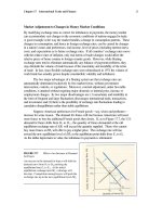
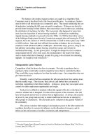
FIGURE 15.1 Shift in Demand for Labor
The demand for labor, like all other demand
curves, slopes downward. An increase in the
demand for labor will cause a rightward shift in the
demand curve, from D
1
to D
2
. A decrease will
cause the leftward shift, to D
3
.

The Supply of Labor
The supply of labor is the assumed positive relationship between the real wage rate and
the number of workers (or work hours) offered for employment during a given period,
everything else held constant. The supply curve for labor generally slopes upward. At
higher wage rates, more workers will be willing to work longer hours than at lower wage
rates (see Figure 15.2). If you survey your MBA classmates, for example, you will
probably find that more of them would be willing to work at a job that paid $50 an hour
than would work for $20 an hour. (At $500 an hour, most would be willing to work
without hesitation, aside for a few lawyers and consultants!)
The supply of labor depends on the opportunity cost of a worker’s time. Workers
can do many different things with their time. They can use it to construct mousetraps, to
do other jobs, to go fishing, and so on. Weighing the opportunity cost of each activity,
the worker will allocate his time so that the marginal benefit of an hour spent doing one
thing will equal the marginal benefit of time that could be used elsewhere. Because some
kinds of work are unpleasant, workers will require a wage to make up for the time lost
from leisure activities like fishing. To earn a given wage, a rational worker will give up
the activities he values least. To allocate even more time to a job (and give up more
valuable leisure-time activities), a worker will require a higher wage.
Chapter 15 Competitive and Monopsonistic
Labor Markets



5
Given this cost-benefit tradeoff, employers who want to increase production have
two options. They can hire additional workers or ask the same workers to work longer
hours. Those who are currently working for $20 an hour must value time spent elsewhere
at less than $20 an hour. To attract other workers, people who value their time spent
elsewhere at more than $20 an hour, employers will have to raise the wage rate, perhaps

to $22 an hour. To convince current workers to put in longer hours – to give up more
attractive alternative activities – employers will also have to raise wage rates. In either
case, the labor supply curve slopes upward. More labor is supplied at higher wages.

____________________________________
Figure 15.2 Shift in the Supply of Labor
The supply curve for labor slopes upward. An
increase in the supply of labor will cause a rightward
shift in the supply curve from S
1
to S
2
. A decrease in
the supply of labor will cause a leftward shift in the
supply curve, from S
1
to S
3
.
____________________________________





The supply curve for labor will shift if the value of employees’ alternatives
changes. For example, if the wage that mousetrap makers can earn in toy production
goes up, the value of their time will increase. The supply of labor to the mousetrap
industry should then decrease, shifting upward and to the left from S
1

to S
3
, in Figure
15.2. This shift in the labor supply curve means that less labor will be offered at any
given wage rate, in a particular labor market. To hire the same quantity of labor—to keep
mousetrap makers from going over to the toy industry—the employer must increase the
wage rate.
The same general effect will occur if workers’ valuation of their leisure time
changes. Because most people attach a high value to time spent with their families on
holidays, employers who want to maintain operations then generally have to pay a
premium for workers’ time. The supply curve for labor on holidays lies above and to the
left of the regular supply curve. Conversely, if for any reason the value of workers’
alternatives decreases, the supply curve for labor will shift down to the right. If wages in
the toy industry fall, for instance, more workers will want to move into the mousetrap
business, increasing the labor supply in the mousetrap market.


Chapter 15 Competitive and Monopsonistic
Labor Markets



6
Equilibrium in the Labor Market
A competitive market is one in which neither the individual employer nor the individual
employee has the power to influence the wage rate. Such a market is shown in Figure
15.3. Given the supply curve S and the demand curve D, the wage rate will settle at W
1
,
and the quantity of labor employed will be Q

2
. At that combination, defined by the
intersection of the supply and demand curves, those who are willing to work for wage W
1

can find jobs.
The equilibrium wage rate is determined much as the prices of goods and services
are established. At a wage rate of W
2
, the quantity of labor employers will hire is Q
1
,
whereas the quantity of workers willing to work is Q
3
. In other words, at that wage rate a
surplus of labor exists. Note that all the workers in this surplus except the last one are
willing to work for less than W
2
. That is, up to Q
3
, the supply curve lies below W
2
. The
opportunity cost of these workers’ time is less than W
2
. They can be expected to accept a
lower wage, and over time they will begin to offer to work for less than W
2
. Other
unemployed and employed workers must then compete by accepting still lower wages.

In this manner the wage rate will fall toward W
1
. In the process, the quantity of labor that
employers can afford to hire will expand from Q
1
toward Q
2
.

___________________________________
FIGURE 15.3 Equilibrium in the Labor Market
Given the supply and demand curves for labor S and
D, the equilibrium wage will be W
1
, and the
equilibrium quantity of labor hired, Q
2
. If the wage
rate rises to W
2
, a surplus of labor will develop,
equal to the difference between Q
3
and Q
1
.

Meanwhile, the falling wage rate will convince some workers to take another
opportunity, such as going fishing or getting another job. As they withdraw from the
market, the quantity of labor supplied will decline from Q
3
toward Q
2
. The quantity
supplied will meet the quantity demanded—and eliminate the surplus—at a wage rate of
W
1
.
In practice, the money wage rate—the number of dollars earned per hour—may
not fall. Instead, the general price level may increase while the money wage rate remains
constant. But the real wage rate—that is, what the money wage rate will buy—still falls,
producing the same general effects: fewer laborers willing to work, and more workers
demanded by employers. When economists talk about wage increases or decreases, they
mean changes in the real wage rate, or in the purchasing power of a worker’s paycheck.