Computational Plasticity- P2
Bạn đang xem bản rút gọn của tài liệu. Xem và tải ngay bản đầy đủ của tài liệu tại đây (1.02 MB, 30 trang )
Towards a Model for Large Strain Anisotropic Elasto-Plasticity 23
a principal strain direction
or principal orthotropy di-
rection in the final spatial
configuration
a principal strain
direction in the trial
unrotated configuration
a principal orthotropy
direction in the trial
unrotated configuration
a principal strain direction
or principal orthotropy di-
rection in the final unrotated
configuration
Fig. 1. Configurations involved in the stress-integration algorithm
where M is the mixed hardening parameter,
2
3
H :=
¯
h (1 − M) is the effec-
tive kinematic hardening modulus and K :=
¯
hM is the isotropic hardening
modulus. The parameter
¯
h plays the role of effective hardening modulus. The
parameter K
w
is a hardening for couple-stresses. Eq.(51) corresponds to a
SPM description of hardening, see Reference [43]. However, for constant
¯
h it
coincides with the SPS method. In (51) we have included the possibility of
anisotropic kinematic hardening through the use of an anisotropy tensor H,
similar to A
d
. The tensor H
←−
, rotates at the speed given by the internal spin
tensor W
H
for similar reasons as those given for the stored energy function.
We define the internal
overstresses as
κ :=
∂ψ
∂ζ
and κ
w
:=
∂ψ
∂ξ
(53)
Hence,
κ =
∂ψ
∂ζ
=
∂H
∂ζ
= Kζ and κ
w
=
∂ψ
∂ξ
=
∂H
∂ξ
= K
w
ξ (54)
or
˙κ =
∂
2
ψ
∂ζ
2
˙
ζ =
∂
2
H
∂ζ
2
˙
ζ = K
˙
ζ and ˙κ
w
=
∂
2
ψ
∂ξ
2
˙
ξ =
∂
2
H
∂ξ
2
˙
ξ = K
w
˙
ξ (55)
the internal backstress as
B
←−
s
=
∂ψ
∂ E
←−
i
apr
=
∂H
∂ E
←−
i
apr
= H H
←−
: E
←−
i
(56)
Then, the derivative of the hardening potential is
˙
H = B
←−
s
:
˙
E
←−
i
+
1
2
H E
←−
i
:
˙
H
←−
: E
←−
i
+ κ
˙
ζ + κ
w
˙
ξ (57)
We define
Please purchase PDF Split-Merge on www.verypdf.com to remove this watermark.
24 F.J. Mont´ans and K.J. Bathe
and following the same steps as for the stored energy function
1
2
H E
←−
i
:
˙
H
←−
: E
←−
i
= B
←−
w
: W
←−
H
(58)
where B
←−
w
is a skew tensor defined as
B
←−
w
:= E
←−
i
B
←−
s
− B
←−
s
E
←−
i
(59)
Finally we have
˙
H = B
←−
s
:
˙
E
←−
i
+ B
←−
w
: W
←−
H
+ κ
˙
ζ + κ
w
˙
ξ
= B
s
: L
←−
E
i
+ B
w
: W
H
+ κ
˙
ζ + κ
w
˙
ξ (60)
However, we note that equations (51), (54) and (56) may not be formally
adequate because they are defined in terms of total internal strains and, as
the plastic strains, they are path dependent. Hence directly assuming (60),
(55) and the rate form of (56) is more appropriate, and (51) should be taken
just for motivation purposes. Furthermore, Equation (33) should formally be
assumed in rate form, and in the derivations to follow only the rate form will
be used.
4 Mapping Tensors from Quadratic to Logarithmic
Strain Space
In large strain plasticity, logarithmic strain measures frequently yield simple
and natural descriptions. Of course, these strains may be used in any config-
uration simply using the proper stretch tensor to obtain them. The following
relationship holds:
E
e
= R
eT
e
e
R
e
with E
e
=lnU
e
, e
e
=lnV
e
(61)
Hence, it is noted that for logarithmic strain tensors, the push-forward and
pull-back operations are performed with the rotation part of the deformation
gradient alone. One may say that the stress-free configuration and the “unro-
tated” configuration are coincident in the logarithmic strain space. Obviously,
since the logarithmic strain tensors and the Almansi and Green strains are
all unique for a given deformation gradient, there exist a one-to-one mapping
between them. For example
E
e
= M
E
A
: A
e
(62)
where if the spectral forms of the strain tensors are
E
e
=
3
i=1
ln λ
e
i
N
i
⊗ N
i
, A
e
=
3
i=1
1
2
λ
e 2
i
− 1
N
i
⊗ N
i
(63)
Please purchase PDF Split-Merge on www.verypdf.com to remove this watermark.
Towards a Model for Large Strain Anisotropic Elasto-Plasticity 25
M
E
A
can be written as
M
E
A
=
3
i=1
2lnλ
e
i
λ
e 2
i
− 1
N
i
⊗ N
i
⊗ N
i
⊗ N
i
(64)
as it is straightforward to verify. Conversely
M
A
E
=
3
i=1
λ
e 2
i
− 1
2lnλ
e
i
N
i
⊗ N
i
⊗ N
i
⊗ N
i
(65)
is such that A
e
= M
A
E
: E
e
. In a similar way, there is a one-to-one mapping
between the deformation rate tensor and the time-derivative of the logarithmic
strains. These mapping tensors may be found to be (see Reference [51])
M
˙
E
D
=
∂E
e
∂A
e
=
3
i=1
1
λ
e 2
i
M
i
⊗ M
i
+
3
i=1
j=i
2
ln λ
e
j
− ln λ
e
i
λ
e 2
j
− λ
e 2
i
M
i
s
M
j
(66)
and
M
D
˙
E
=
∂A
e
∂E
e
=
3
i=1
λ
e 2
i
M
i
⊗ M
i
+
3
i=1
j=i
1
2
λ
e 2
j
− λ
e 2
i
ln λ
e
j
− ln λ
e
i
M
i
s
M
j
(67)
where
M
i
:= N
i
⊗ N
i
(68)
M
i
s
M
j
:=
1
4
(N
i
⊗ N
j
+ N
j
⊗ N
i
) ⊗ (N
i
⊗ N
j
+ N
j
⊗ N
i
) ≡ M
j
s
M
i
(69)
These tensors have major and minor symmetries and represent the one-to-one
mappings relating deformation rates as
˙
E
e
= M
˙
E
D
: D
e
and D
e
= M
D
˙
E
:
˙
E
e
(70)
respectively. Furthermore, in the rotation-frozen configuration
˙
E
←−
e
= M
←−
˙
E
D
: D
←−
e
and D
←−
e
= M
←−
D
˙
E
:
˙
E
←−
e
(71)
Also, in the stress-free configuration
L
←−
E
e
= M
˙
E
D
: L
←−
A
e
and L
←−
A
e
= M
D
˙
E
: L
←−
E
e
(72)
For future use, we define two fourth order mapping tensors
W
←−
M
:=
1
2
C
←−
e
3
· M
←−
˙
E
D
− C
←−
e
4
· M
←−
˙
E
D
(73)
Please purchase PDF Split-Merge on www.verypdf.com to remove this watermark.
26 F.J. Mont´ans and K.J. Bathe
and
S
←−
M
:=
1
2
C
←−
e
3
· M
←−
˙
E
D
+ C
←−
e
4
· M
←−
˙
E
D
(74)
where by
n
·
we imply the contraction of the n − index of the fourth order
tensor with the second index of the second order tensor. Then, it can be shown
that if we define
K
←−
:= S
←−
: M
←−
D
˙
E
so that S
←−
=: K
←−
: M
←−
˙
E
D
(75)
we obtain
Ξ
←−
:= C
←−
e
S
←−
= C
←−
e
K
←−
: M
←−
˙
E
D
= K
←−
:
S
←−
M
+ W
←−
M
(76)
and
K
←−
w
:= K
←−
: W
←−
M
= E
←−
e
K
←−
− K
←−
E
←−
e
≡ Ξ
w
(77)
Ξ
←−
s
= K
←−
: S
←−
M
(78)
stress tensor T , see also
below, and hence the conversion to the symmetric part of the Mandel stress
tensor Ξ
s
is given by Equation (78).
5 Dissipation Inequality
The stress power in the reference volume may be expressed in the intermediate
configuration as
P≡S : L = S :(L
e
+ C
e
L
p
) (79)
= S :(D
e
+ W
e
)+S : C
e
(D
p
+ W
p
) (80)
where S is the pull-back of the Kirchhoff stress τ to the stress-free configura-
tion. Since S is symmetric the product S : W
e
= 0, i.e. the modified elastic
spin (which also contains the rigid-body spin) produces no work. Thus, in a
rotationally-frozen configuration we are left with
P≡ S
←−
: L
←−
= K
←−
:
˙
E
←−
e
+ S
←−
: C
←−
e
D
←−
p
+ W
←−
p
(81)
where we used (71) and (75). Alternatively, in the stress-free configuration
S : L = K : L
←−
E
e
+ S : C
e
(D
p
+ W
p
) (82)
= K : L
←−
E
e
+ C
e
S :(D
p
+ W
p
) (83)
Using Ξ = C
e
S, the stress power can be written as
S : L = K : L
←−
E
e
+(Ξ
s
+ Ξ
w
):(D
p
+ W
p
)
= K : L
←−
E
e
+ Ξ
s
: D
p
+ Ξ
w
: W
p
(84)
The tensor K is actually the generalized K irchhoff
Please purchase PDF Split-Merge on www.verypdf.com to remove this watermark.
Towards a Model for Large Strain Anisotropic Elasto-Plasticity 27
Thus, the symmetric Mandel stress tensor produces power on the modified
plastic strain rate, whereas the skew-symmetric Mandel tensor produces power
on the modified plastic spin. This last work is due to the kinematic cou-
pling produced by the Lee decomposition and the possible rotation of elastic
anisotropy axes. In the case of isotropy or deformation through the orthotropy
axes, the term vanishes. Neglecting the effect of temperature, the dissipation
inequality from the second law of the thermodynamics is
˙
D = P−
˙
ψ ≥ 0 (85)
where
˙
ψ is the free energy function rate, assumed to be
˙
ψ =
˙
W +
˙
H.Thus
using (49) and (60)
˙
ψ = T : L
←−
E
e
+ T
w
: W
A
+ B
s
: L
←−
E
i
+ B
w
: W
H
+ κ
˙
ζ + κ
w
˙
ξ (86)
and
˙
D =(K − T ):L
←−
E
e
+ Ξ
s
: D
p
+ Ξ
w
: W
p
−T
w
: W
A
− B
s
: L
←−
E
i
− B
w
: W
H
− κ
˙
ζ − κ
w
˙
ξ ≥ 0 (87)
Since the equality must hold for pure elastic deformations,
T = K (88)
and, in consequence,
T
w
= K
w
≡ Ξ
w
(89)
The reduced (plastic) dissipation inequality is now
˙
D
p
= Ξ
s
: D
p
+ Ξ
w
: W
d
− B
s
: L
←−
E
i
− B
w
: W
H
− κ
˙
ζ − κ
w
˙
ξ ≥ 0 (90)
where we defined the dissipative spin tensor in the unrotated configuration as
W
d
:= W
p
− W
A
(91)
We note that if W
p
= W
A
then the skew part of the Mandel stress tensor does
not contribute to the dissipation function. On the other hand, since W
A
is
assumed to be a function of W
p
,ifW
p
= 0 then W
A
= 0 and no dissipation
takes place either due to the skew part of the Mandel stress tensor. We will
assume that the following relationship holds
W
A
= ρW
p
(92)
where ρ is a material scalar parameter. Then
W
d
=(1− ρ) W
p
(93)
We assume now –without loss of generality– that the elastic region is
enclosed by two yield functions f
s
(Ξ
s
, B
s
,κ)andf
w
(Ξ
w
, B
w
,κ
w
), the La-
grangian for the constrained problem is L =
˙
D
p
−
˙
tf
s
− ˙γf
w
, where
˙
t and ˙γ
Please purchase PDF Split-Merge on www.verypdf.com to remove this watermark.
28 F.J. Mont´ans and K.J. Bathe
are the consistency parameter increments. Note also that L
←−
E
i
≡ D
i
.Ifwe
claim that the principle of maximum dissipation holds, the stress and other
internal variables are such that ∇L = 0, i.e. for the yield function expressions
given
∇L =0⇒
⎧
⎪
⎪
⎪
⎪
⎪
⎪
⎪
⎨
⎪
⎪
⎪
⎪
⎪
⎪
⎪
⎩
∂L
∂Ξ
s
=0 ⇒ D
p
=
˙
t
∂f
s
∂Ξ
s
and
∂L
∂Ξ
w
=0 ⇒ W
d
=˙γ
∂f
w
∂Ξ
w
∂L
∂B
s
=0 ⇒L
←−
E
i
= −
˙
t
∂f
s
∂B
s
and
∂L
∂B
w
=0 ⇒ W
H
= − ˙γ
∂f
w
∂B
w
∂L
∂κ
=0 ⇒
˙
ζ = −
˙
t
∂f
s
∂κ
and
˙
ξ = − ˙γ
∂f
w
∂κ
w
(94)
These expressions are the associated flow and hardening rules for general
elastoplasticity at finite strains. It is noted that if, as usual, the enclosure of the
elastic region for the symmetric part is expressed in the form of f
s
(Ξ
s
− B
s
...)
then for associative plasticity the following relationship is automatically en-
forced
L
←−
E
i
≡ D
i
= D
p
(95)
Furthermore, W
i
does not affect the dissipation function and can be freely
(95), and assuming that internal vari-
ables rotate as the plastic variables, we will set
W
i
= W
p
(96)
and, as a consequence
X
i
= X
p
(97)
The loading/unloading (complementary) Kuhn-Tucker conditions are, as
usual
˙
t ≥ 0, f
s
≤ 0and
˙
tf
s
≡ 0 (98)
˙γ ≥ 0, f
w
≤ 0 and ˙γf
w
≡ 0 (99)
and the consistency conditions are
˙
t
˙
f
s
≡ 0 and ˙γ
˙
f
w
≡ 0 (100)
The formulations presented herein and in Reference [44] show some simi-
larities with some other works, see for example References [18, 20, 45–48], but
there are also some significant differences; in particular we are using logarith-
mic strains in an incremental form.
6 Yield Functions
There is still much experimental work needed to establish the elastic domain
and yield functions for the symmetric and skew parts of the Mandel stress
tensor. From the current experimental evidence it is difficult to infer sound
prescribed. In view of Equation
Please purchase PDF Split-Merge on www.verypdf.com to remove this watermark.
Towards a Model for Large Strain Anisotropic Elasto-Plasticity 29
data about a macroscopic (continuum) elastic domain for the skew part of the
Mandel stress tensor, and for the plastic spin evolution. Hence, at this point a
“reasonable” proposition is necessary. An ad hoc extension of the small strains
theory without plastic spin follows.
6.1 Yield Function for the Symmetric Part
For the symmetric part of the Mandel stress tensor the well-known Hill’s
quadratic yield criterion is assumed to hold, i.e. the yield function for Ξ
s
is
given by the expression (see for example Reference [1])
f
s
:=
3
2κ
2
(Ξ
s
− B
s
):A
p
s
:(Ξ
s
− B
s
) − 1 = 0 (101)
where A
p
s
is the plastic anisotropy tensor which in this work we assume to
have the same preferred anisotropy directions as the elastic anisotropy tensor.
Given this function, the specific values of the internal variable increments are
obtained from Equations (94) and (95) as
D
i
= D
p
=
˙
t
∂f
s
∂Ξ
s
=
3
κ
2
A
p
s
:(Ξ
s
− B
s
)
˙
t (102)
The internal isotropic variable rate is obtained as
˙
ζ = −
˙
t
∂f
s
∂κ
=
2
κ
(f
s
+1)
˙
t (103)
which, at the yield condition (f
s
= 0) takes the value
˙
ζ =2
˙
t/κ. The physical
meaning of
˙
ζ is the effective plastic strain rate, see Reference [1].
6.2 Yield Function for the Skew Part
For the skew part, in this work we consider the simplest possible yield function,
of the Mises type
f
w
= Ξ
w
−
√
2κ
w
(104)
where κ
w
is the allowed yield value, which may take the value of zero. From
Equation (94), the specific flow variables take the form
W
d
=˙γ
∂f
w
∂Ξ
w
=˙γ
ˆ
Ξ
w
(105)
˙
ξ = − ˙γ
∂f
w
∂κ
w
=
√
2˙γ (106)
where we defined the “direction”
ˆ
Ξ
w
:= Ξ
w
/Ξ
w
. The physical meaning of
˙
ξ is the effective dissipative rotation rate. Using Equations (92) and (93) we
obtain
W
p
=
1
(1 − ρ)
˙γ
ˆ
Ξ
w
and W
A
=
ρ
(1 − ρ)
˙γ
ˆ
Ξ
w
(107)
Please purchase PDF Split-Merge on www.verypdf.com to remove this watermark.
30 F.J. Mont´ans and K.J. Bathe
One important consequence of the function f
w
defined in Equation (104)
and the expression (107
2
)isthatif1>ρ>0 then W
A
and Ξ
w
≡ T
w
have
the same direction. But as noted just after Equation (44), the term T
w
: W
A
should be negative. Hence possible values are ρ>1andρ<0. If ρ>1 then
the term T
w
: W
A
is negative and W
p
and W
A
have the same direction.
If ρ<0 then the term T
w
: W
A
is also negative and W
p
and W
A
have
opposite direction. The actual rotation direction is not only determined by ρ,
but also by the elastic anisotropy tensor because its shape may change the
direction of Ξ
w
.
6.3 Coupling of Symmetric and Skew Parts
The yield function Equation (104) would mean an instantaneous rotation once
Ξ
w
is over the allowed value
√
2κ
w
. However this is not consistent with
experiments, in which progressive rotations are observed. Aside, in mechanics
of single crystals this rotation is not independent of the ordinary (symmetric)
plastic flow (Schmid’s law). Hence, in this work we propose a viscoplasticity-
like flow for the skew part in which the effective plastic strain plays the role
of the time variable. This proposed expression is
˙
ξ =
<f
w
>
η
m
˙
ζ (108)
where < · > is the Macauley bracket function, η is the “viscosity” material
parameter with units of (couple-)stress and m is another material parameter.
Hence, f
w
may have values greater than zero which relax with plastic flow. In
terms of consistency parameters, Equation (108) may be written as
˙γ =
√
2
κ
<f
w
>
η
m
˙
t (109)
Hence, ˙γ is zero if either f
w
≤ 0or
˙
t =0.
7 Numerical Example
In order to test the capabilities of the present theory in modelling the rotation
of the anisotropy directions, we have carried out some numerical experiments.
In these numerical tests, we aim for predictions of the experimental results
reported in Reference [32]. In these experiments, a rotation of the material
symmetry was observed when a steel sheet is strained in a direction that forms
an angle θ with the rolling or prestrain direction. Details of the experiments are
given in Reference [32]. Only small changes in the shape of the yield function
were observed and hence the shape of the yield function can be assumed to
remain constant, see also Reference [33].
Please purchase PDF Split-Merge on www.verypdf.com to remove this watermark.
Towards a Model for Large Strain Anisotropic Elasto-Plasticity 31
However, unfortunately, in Reference [32] only the measured plastic ani-
sotropy and its evolution are reported. Since our theory includes and indeed
uses elastic anisotropy, we need to assume elastic anisotropy parameters. In
a uniaxial test, a relevant degradation of Young’s modulus and a variation of
Poisson’s ratio in the test direction has been reported [49]. Elastic anisotropy
has also been measured in rolled steel, brass and aluminum, see for example
[50]. We therefore assume the following elastic (only slightly anisotropic) mate-
rial parameters: E
a
=2.04×10
11
Pa, E
b
=2.03×10
11
Pa, E
c
=2.10×10
11
Pa,
ν
ab
=0.3, ν
ac
=0.3, ν
bc
=0.3, and G
ab
=0.82 × 10
11
Pa. The yield stress κ
0
and Hill’s yield function parameters have been reported in Reference [32],
i.e. f =0.3613, h =0.4957, g =0.3535 and we used N =1.175 and
κ
0
=23× 10
7
Pa. The hardening has been considered as isotropic according
to the formula κ = κ
∞
− (κ
∞
− κ
0
)exp(−δζ)+
¯
hζ, for which the constants
have been deduced from the experimental data,
¯
h =3.5×10
8
Pa, κ
∞
=1.2κ
0
,
δ = 30. We also used the parameters κ
w
=0,m =2,ρ = −2andη = 600 Pa.
All these parameters should really be chosen based on experimental results.
However, we used the mentioned values and only adjusted η to match the ex-
perimental data. Details of the numerical implementation of the theory may
be found in Reference [51].
The Young’s modulus and the yield stress in the different directions, as
well as their evolution are shown in Figure 2. In this figure we also compare
the predicted yield stresses with the experimental data for the case of the ap-
plied load at θ =30
o
to the rolling direction. Figure 3 compares experimental
data and computed results for θ =30
o
,45
o
and 60
o
. Of course, different
elastic anisotropy constants (obtained experimentally) would change the pre-
dictions, but then also the material parameters η, ρ and m should be based on
experimental results. An important feature of our formulation is that different
rotation rates are obtained for different angles, and the predictions may not be
symmetric for 30 and 60 degrees —in accordance with experimental results—
even though the yield function is almost symmetric about the direction 44.7
degrees with the rolling direction. This is due to the selected shape for the
anisotropy tensors.
8 Conclusions
We presented our research towards a model for anisotropic elasto-plasticity.
The model shall represent possible anisotropic elasticity, anisotropic yield sur-
faces, hardening and the rotation of the elastic and plastic orthotropy direc-
tions during plastic flow. Both the continuum and time integration incremental
formulations are simultaneously derived since incremental formulations give
some insight into the continuum formulation. The model and the integration
algorithm are derived using the multiplicative Lee decomposition of the total
deformation gradient into an elastic and a plastic part. However, no total plas-
Please purchase PDF Split-Merge on www.verypdf.com to remove this watermark.
32 F.J. Mont´ans and K.J. Bathe
2.02
2.03
2.04
2.05
2.06
2.07
2.08
2.09
2.1
x10
11
Young's modulus E [Pa]
(a)
0
20
40
60
80
100
120
140
160
180
2.2
2.4
2.6
2.8
3
3.2
3.4
3.6
x10
8
a
Yield stress k [Pa]
(c)
120
140
e
Prediction:
x
=0%
x
=2%
x
=5%
x
= 10%
e
e
e
e
x
=0%
e
x
=2%
e
x
=5%
e
x
= 10%
Kim & Yin exp.:
x
Y
(RD)
q
Pred. & exp.
a
b
(b)
0
20
40
60
80
a
100
120 140 160 180
Fig. 2. (a) Prediction of the evolution of the Young’s modulus profile at different
spatial strains e
x
for a uniaxial load at an angle of θ =30
o
with respect to the rolling
direction (RD). (b) Angles involved in the example. Angle of the uniaxial load with
the rolling direction (θ), angle of the principal direction a with the uniaxial load
(β) —initially β = θ—, angle of the Young’s modulus and yield stress shown in the
curves with the uniaxial load (α). (c) Comparison of the experimental data of [32]
with the prediction of the evolution of the yield stress profile at different spatial
strains e
x
for a plane stress load at an angle of θ =30
o
with respect to the rolling
direction
Please purchase PDF Split-Merge on www.verypdf.com to remove this watermark.
Towards a Model for Large Strain Anisotropic Elasto-Plasticity 33
0
0.01
0.02
0.03
0.04
0.05
0.06
0.07
0.08
0.09
0.1
0
20
40
60
80
100
b
(a)
Kim & Yin experiments, q = 30º, q = 45º, q = 60º
Prediction for q = 30º
Prediction for q = 45º
Prediction for q = 60º
2
2.2
2.4
2.6
2.8
3
3.2
x10
8
t
x
[Pa ]
(b)
2
4
6
8
10
|| t
w
||
0 0.01 0.02 0.03 0.04 0.05 0.06 0.07 0.08 0.09 0.1
0.05
0
0.01
0.02
0.030.04
0.06
0.070.080.1 0.09
e
x
e
x
x10
3
[Pa ]
Fig. 3. (a) Prediction for the evolution of the principal orthotropy directions and
comparison with the experimental values of Reference [32]. (b) Uniaxial stress and
couple-stress evolutions
tic deformation measure is used. Plastic deformations and plastic rotations are
considered only incrementally.
The stresses are directly obtained from the logarithmic elastic strains, with
the model assuming linear elastic anisotropy and moderate elastic strains, but
accounting for possible large plastic strains.
The model presented offers, in particular, possibilities to simulate the rota-
tion of the material axes observed in experiments on anisotropic elasto-plastic
materials, and as an example good correlation to the experimental data of
Kim and Yin has been obtained.
However, clearly, the model must be studied much more. The sensitivity
of the model predictions with respect to the model parameters needs to be
identified, and comparisons of computed solutions with test data for many
more and varied material tests need to be obtained. These studies will also
identify the limitations of the model and whether the model could be simplified
without significant loss of predictive capability.
Please purchase PDF Split-Merge on www.verypdf.com to remove this watermark.
34 F.J. Mont´ans and K.J. Bathe
References
1. Koji´c M, Bathe KJ (2005) Inelastic analysis of solids and structures. Springer-
Verlag, New York
2. Bathe KJ (1996) Finite element procedures. Prentice-Hall, New Jersey
3. Sim´o JC (1988) A framework for finite strain elastoplasticity based on maximum
plastic dissipation and the multiplicative decomposition. Part I: Continuum for-
mulation. Comp Meth Appl Mech Engrng 66: 199-219. Part II: Computational
aspects. Comp Meth Appl Mech Engrng 68: 1-31
4. Sim´o JC, Hughes TJR (1998) Computational inelasticity. Springer-Verlag, New
York
5. Bathe KJ, Ramm E, Wilson EL (1975) Finite element formulations for large
deformation dynamic analysis. Int J Num Meth Engrg 9: 353-386
6. Koji´c M, Bathe KJ (1987) Studies of finite element procedures—Stress solution
of a closed elastic strain path with stretching and shearing using the updated
Lagrangian Jaumann formulation. Comp Struct 26: 175-179
7. Lee EH (1969) Elastic-plastic deformations at finite strains. J Appl Mech ASME
36: 1-6
8. Lee EH, Liu DT (1967) Finite-strain elastic-plastic theory with application to
plane wave analysis. J Appl Phys 38: 19-27
9. Bilby BA, Bullough R, Smith E (1955) Continuous distributions of dislocations:
A new application of the methods of Non-Riemannian Geometry. Proc Roy Soc
London Ser A 231: 263-273
10. Weber G, Anand L (1990) Finite deformation constitutive equations and a time
integration procedure for isotropic hyperelastic-viscoplastic solids. Comp Meth
Appl Mech Engrg 79: 173-202
11. Eterovi´c AL, Bathe KJ (1990) A hyperelastic-based large strain elasto-plastic
constitutive formulation with combined isotropic-kinematic hardening using the
logarithmic stress and strain measures. Int J Num Meth Engrg 30: 1099-1114
12. Sim´o JC (1992) Algorithms for multiplicative plasticity that preserve the form of
the return mappings of the infinitesimal theory. Comp Meth Appl Mech Engrg
99: 61-112
13. Peri´c D, de Souza EA (1999) A new model for Tresca plasticity at finite strains
with an optimal parametrization in the principal space. Comp Meth Appl Mech
Engrg 171: 463-489
14. Mont´ans FJ, Bathe KJ (2003) On the stress integration in large strain elasto-
plasticity. In: Bathe KJ (ed) Computational fluid and solid mechanics 2003.
Elsevier, Oxford
15. Mont´ans FJ, Bathe KJ (2005) Computational issues in large strain elasto-
plasticity: An algorithm for mixed hardening and plastic spin. Int J Num Meth
Engrg 63: 159-196
16. Cuiti˜no A, Ortiz M (1992) A material-independent method for extending stress
update algorithms from small strain plasticity to finite plasticity with multi-
plicative kinematics. Engrg Comp 9: 437-451
17. Borja RI, Tamagnini C (1998) Cam–Clay plasticity, Part III: Extension of the
infinitesimal model to include finite strains. Comp Meth Appl Mech Engrg 155,
77-95
18. Papadopoulus P, Lu J (1998) A general framework for the numerical solution
of problems in finite elasto-plasticity. Comp Meth Appl Mech Engrg 159: 1-18
Please purchase PDF Split-Merge on www.verypdf.com to remove this watermark.