Operations management heizer 6e moda

Operations
Management

Module A –
Decision-Making Tools
PowerPoint presentation to accompany
Heizer/Render
Principles of Operations Management, 6e
Operations Management, 8e

© 2006
Prentice
Hall, Inc. Hall, Inc.
©
2006
Prentice

A–1


Outline
 The Decision Process in
Operations
 Fundamentals of Decision Making
 Decision Tables

© 2006 Prentice Hall, Inc.

A–2

Outline – Continued
 Types of Decision-Making
Environments
 Decision Making Under Uncertainty
 Decision Making Under Risk
 Decision Making Under Certainty
 Expected Value of Perfect
Information (EVPI)

© 2006 Prentice Hall, Inc.

A–3


Outline – Continued
 Decision Trees
 A More Complex Decision Tree
 Using Decision Trees in Ethical
Decision Making

© 2006 Prentice Hall, Inc.

A–4


Learning Objectives
When you complete this module, you
should be able to:
Identify or Define:
 Decision trees and decision

tables
 Highest monetary value
 Expected value of perfect
information
 Sequential decisions
© 2006 Prentice Hall, Inc.

A–5


Learning Objectives
When you complete this module, you
should be able to:
Describe or Explain:
 Decision making under risk
 Decision making under
uncertainty
 Decision making under
certainty

© 2006 Prentice Hall, Inc.

A–6


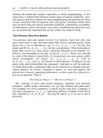
The Decision Process in
Operations
1. Clearly define the problems and the
factors that influence it
2. Develop specific and measurable

objectives
3. Develop a model
4. Evaluate each alternative solution
5. Select the best alternative
6. Implement the decision and set a
timetable for completion
© 2006 Prentice Hall, Inc.

A–7


Fundamentals of
Decision Making
1. Terms:
a. Alternative—a course of action or
strategy that may be chosen by the
decision maker
b. State of nature—an occurrence or a
situation over which the decision
maker has little or no control

© 2006 Prentice Hall, Inc.

A–8


Fundamentals of
Decision Making
2. Symbols used in a decision tree:
a. —decision node from which one

of several alternatives may be
selected
b. —a state-of-nature node out of
which one state of nature will occur

© 2006 Prentice Hall, Inc.

A–9


Decision Tree Example
A decision node

A state of nature node
Favorable market

ct
u
r
st lant
n
Co ge p
lar
Construct
small plant

Unfavorable market

Do
no

thi
ng

Unfavorable market

Favorable market

Figure A.1
© 2006 Prentice Hall, Inc.

A – 10


Decision Table Example
Alternatives
Construct large plant
Construct small plant
Do nothing

State of Nature
Favorable Market
Unfavorable Market
$200,000
–$180,000
$100,000
–$ 20,000
$
0
$
0

Table A.1

© 2006 Prentice Hall, Inc.

A – 11


Decision-Making
Environments
 Decision making under uncertainty
 Complete uncertainty as to which
state of nature may occur

 Decision making under risk
 Several states of nature may occur
 Each has a probability of occurring

 Decision making under certainty
 State of nature is known
© 2006 Prentice Hall, Inc.

A – 12


Uncertainty
1. Maximax
 Find the alternative that maximizes
the maximum outcome for every
alternative

 Pick the outcome with the maximum
number
 Highest possible gain

© 2006 Prentice Hall, Inc.

A – 13


Uncertainty
2. Maximin
 Find the alternative that maximizes
the minimum outcome for every
alternative
 Pick the outcome with the minimum
number
 Least possible loss

© 2006 Prentice Hall, Inc.

A – 14


Uncertainty
3. Equally likely
 Find the alternative with the highest
average outcome
 Pick the outcome with the maximum
number
 Assumes each state of nature is

equally likely to occur

© 2006 Prentice Hall, Inc.

A – 15


Uncertainty Example
States of Nature
Alternatives

Favorable
Market

Unfavorable
Market

Construct
large plant

$200,000

-$180,000

Construct
small plant

$100,000
$0

Do nothing

Maximum
in Row

Row
Average

$200,000 -$180,000

$10,000

-$20,000

$100,000

-$20,000

$40,000

$0

$0

$0

$0

Maximax

1.
2.
3.

Minimum
in Row

Maximin

Equally
likely

Maximax choice is to construct a large plant
Maximin choice is to do nothing
Equally likely choice is to construct a small plant

© 2006 Prentice Hall, Inc.

A – 16


Risk
 Each possible state of nature has an
assumed probability
 States of nature are mutually exclusive
 Probabilities must sum to 1
 Determine the expected monetary value
(EMV) for each alternative

© 2006 Prentice Hall, Inc.

A – 17


Expected Monetary Value
EMV (Alternative i) = (Payoff of 1st state of
nature) x (Probability of 1st
state of nature)
+ (Payoff of 2nd state of
nature) x (Probability of 2nd
state of nature)
+…+ (Payoff of last state of
nature) x (Probability of
last state of nature)

© 2006 Prentice Hall, Inc.

A – 18


EMV Example
Table A.3

States of Nature
Favorable
Market

Unfavorable
Market

Construct large plant (A1)

$200,000

-$180,000

Construct small plant (A2)

$100,000

-$20,000

Do nothing (A3)

$0

$0

Probabilities

.50

.50

Alternatives

1. EMV(A1) = (.5)($200,000) + (.5)($180,000) = $10,000
2. EMV(A2) = (.5)($100,000) + (.5)($20,000) = $40,000
3. EMV(A3) = (.5)($0) + (.5)($0) = $0
© 2006 Prentice Hall, Inc.

A – 19


EMV Example
Table A.3

States of Nature
Favorable
Market

Unfavorable
Market

Construct large plant (A1)

$200,000

-$180,000

Construct small plant (A2)

$100,000

-$20,000

Do nothing (A3)

$0

$0

Probabilities

.50

.50

Alternatives

1. EMV(A1) = (.5)($200,000) + (.5)($180,000) = $10,000
2. EMV(A2) = (.5)($100,000) + (.5)($20,000) = $40,000
3. EMV(A3) = (.5)($0) + (.5)($0) = $0
© 2006 Prentice Hall, Inc.

Best Option
A – 20


Certainty
 Is the cost of perfect information
worth it?
 Determine the expected value of
perfect information (EVPI)

© 2006 Prentice Hall, Inc.

A – 21

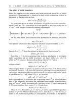
Expected Value of
Perfect Information
EVPI is the difference between the payoff
under certainty and the payoff under risk
EVPI = Expected value – Maximum
under certainty
EMV
Expected value .
(Best outcome or consequence for 1st
under certainty = state of nature) x (Probability of 1st state
of nature)
+ Best outcome for 2nd state of nature)
x (Probability of 2nd state of nature)
+ … + Best outcome for last state of nature)
x (Probability of last state of nature)
© 2006 Prentice Hall, Inc.

A – 22


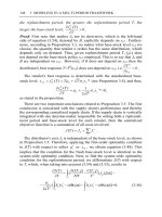
EVPI Example
1. The best outcome for the state of nature
“favorable market” is “build a large
facility” with a payoff of $200,000. The
best outcome for “unfavorable” is “do
nothing” with a payoff of $0.
Expected value = ($200,000)(.50) + ($0)(.50) = $100,000
under certainty

© 2006 Prentice Hall, Inc.

A – 23


EVPI Example
2. The maximum EMV is $40,000, which is
the expected outcome without perfect
information. Thus:
EVPI = Expected value – Maximum
under certainty
EMV
= $100,000 – $40,000 = $60,000
The most the company should pay for
perfect information is $60,000
© 2006 Prentice Hall, Inc.

A – 24


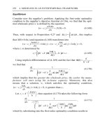
Decision Trees
 Information in decision tables can be
displayed as decision trees
 A decision tree is a graphic display of the
decision process that indicates decision
alternatives, states of nature and their
respective probabilities, and payoffs for
each combination of decision alternative
and state of nature
 Appropriate for showing sequential
decisions

© 2006 Prentice Hall, Inc.

A – 25