Operations management heizer 6e mode

Operations
Management
Module E –
Learning Curves
PowerPoint presentation to accompany
Heizer/Render
Principles of Operations Management, 6e
Operations Management, 8e
© 2006
Prentice
Hall, Inc. Hall, Inc.
©
2006
Prentice

E–1


Outline
 Learning Curves In Services And
Manufacturing
 Applying The Learning Curve
 Arithmetic Approach
 Logarithmic Approach
 Learning-Curve Coefficient Approach

 Strategic Implications of Learning
Curves
 Limitations of Learning Curves
© 2006 Prentice Hall, Inc.

E–2


Learning Objectives
When you complete this module, you
should be able to:
Identify or Define:
 What a learning curve is
 Examples of learning curves
 The doubling concept

© 2006 Prentice Hall, Inc.

E–3


Learning Objectives
When you complete this module, you
should be able to:
Describe or Explain:
 How to compute learning curve
effects
 Why learning curves are important
 The strategic implication of
learning curves

© 2006 Prentice Hall, Inc.

E–4

Learning Curves
 Based on the premise that people and
organizations become better at their
tasks as the tasks are repeated
 Time to produce a unit decreases as
more units are produced
 Learning curves typically follow a
negative exponential distribution
 The rate of improvement decreases
over time
© 2006 Prentice Hall, Inc.

E–5


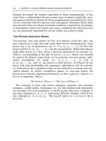
Cost/time per repetition

Learning Curve Effect

0

Number of repetitions (volume)
Figure E.1

© 2006 Prentice Hall, Inc.

E–6

Learning Curves
T x Ln = Time required for the nth unit
where

T
L
n

=
=
=

unit cost or unit time of the first
learning curve rate
number of times T is doubled

First unit takes 10 labor-hours
70% learning curve is present
Fourth unit will require doubling twice — 1 to 2 to 4
Hours required for unit 4 = 10 x (.7)2 = 4.9 hours
© 2006 Prentice Hall, Inc.

E–7


Learning Curve Examples
Improving
Example
Parameters
Model -T Ford Price

production

Cumulative
Parameter
Units produced

LearningCurve
Slope
(%)
86

Aircraft
assembly

Direct labor-hours
per unit

Units produced

80

Equipment
maintenance
at GE

Average time to
replace a group of
parts

Number of

replacements

76

Steel
production

Production worker
labor-hours per unit
produced

Units produced

79

Table E.1
© 2006 Prentice Hall, Inc.

E–8


Learning Curve Examples
Example
Integrated
circuits

Improving
Parameters
Average price per
unit

Cumulative
Parameter
Units produced

LearningCurve
Slope
(%)
72

Hand-held
calculator

Average factory
selling price

Units produced

74

Disk memory
drives

Average price per
bit

Number of bits

76

Heart
transplants

1-year death rates

Transplants
completed

79

Table E.1
© 2006 Prentice Hall, Inc.

E–9


Uses of Learning Curves
Internal:

labor forecasting,
scheduling, establishing
costs and budgets

External: supply chain negotiations
Strategic: evaluation of company and
industry performance,
including costs and pricing

© 2006 Prentice Hall, Inc.

E – 10


Arithmetic Approach
 Simplest approach
 Labor cost declines at a constant rate,
the learning rate, as production doubles
Nth Unit Produced

Hours for Nth Unit

1
2

100.0
80.0 = (.8 x 100)

4
8
16

64.0 = (.8 x 80)
51.2 = (.8 x 64)
41.0 = (.8 x 51.2)

© 2006 Prentice Hall, Inc.

E – 11

Logarithmic Approach
Determine labor for any unit, TN , by
TN = T1(Nb)
where

© 2006 Prentice Hall, Inc.

TN =
time for the Nth unit
T1 =
hours to produce the
first unit
b =
(log of the learning rate)/
(log 2) =
slope of the learning
curve
E – 12


Logarithmic Approach
Determine labor for any unit, TN , by
TN = T1(Nb)
where

Learning
Rate
(%)
time for
the

Nth

TN =
unit b
T1 =
hours to70
produce the
– .515
first unit
75
– .415
b =
(log of the learning
80
– .322
rate)/(log 2)
=
slope of 85
the learning
– .234
curve
90
– .152
Table E.2

© 2006 Prentice Hall, Inc.

E – 13

Logarithmic Example
Learning rate = 80%
First unit took 100 hours
TN = T1(Nb)
T3 = (100 hours)(3b)
= (100)(3log .8/log 2)
= (100)(3–.322)
= 70.2 labor hours
© 2006 Prentice Hall, Inc.

E – 14


Coefficient Approach
TN = T1C
where

© 2006 Prentice Hall, Inc.

TN =
number of laborhours required to produce the
Nth unit
T1 =
number of laborhours required to produce the
first unit
C =
learning-curve
coefficient found in Table E.3
E – 15

Learning-Curve Coefficients
Table E.3

70%

85%

Unit
Number
(N) Time

Unit Time

Total Time

Unit Time

Total Time

1

1.000

1.000

1.000

1.000

2

.700

1.700

.850

1.850

3

.568

2.268

.773

2.623

4

.490

2.758

.723

3.345

5

.437

3.195

.686

4.031

10

.306

4.932

.583

7.116

15

.248

6.274

.530

9.861

20

.214

7.407

.495

12.402

© 2006 Prentice Hall, Inc.

E – 16


Price per unit (log scale)

Industry and Company
Learning Curves

Figure E.2
© 2006 Prentice Hall, Inc.

In
du
C
st
om
ry
pa

pr
ice
ny
co
st
(c)
Loss
(b)

Gross profit
margin

(a)

Accumulated volume (log scale)
E – 17


Coefficient Example
First boat required 125,000 hours
Labor cost = $40/hour
Learning factor = 85%
TN = T1C
T4 = (125,000 hours)(.723)
= 90,375 hours for the 4th boat
90,375 hours x $40/hour = $3,615,000
TN
T4

© 2006 Prentice Hall, Inc.

=
=
=

T1C
(125,000 hours)(3.345)
418,125 hours for all four boats
E – 18


Coefficient Example
Third boat required 100,000 hours
Learning factor = 85%
New estimate for the first boat
100,000
= 129,366 hours
.773

© 2006 Prentice Hall, Inc.

E – 19


Strategic Implications
To pursue a strategy of a steeper curve
than the rest of the industry, a firm can:
1. Follow an aggressive pricing policy
2. Focus on continuing cost reduction
and productivity improvement

3. Build on shared experience
4. Keep capacity ahead of demand

© 2006 Prentice Hall, Inc.

E – 20


Limitations of Learning
Curves
 Learning curves differ from company to
company as well as industry to
industry so estimates should be
developed for each organization
 Learning curves are often based on
time estimates which must be accurate
and should be reevaluated when
appropriate

© 2006 Prentice Hall, Inc.

E – 21


Limitations of Learning
Curves
 Any changes in personnel, design, or
procedure can be expected to alter the
learning curve
 Learning curves do not always apply to

indirect labor or material
 The culture of the workplace, resource
availability, and changes in the process
may alter the learning curve

© 2006 Prentice Hall, Inc.

E – 22