Barriers - Simple European Options
Bạn đang xem bản rút gọn của tài liệu. Xem và tải ngay bản đầy đủ của tài liệu tại đây (243.3 KB, 12 trang )
15
Barriers: Simple European Options
Barrier options are like simple options but with an extra feature which is triggered by the stock
price passing through a barrier. The feature may be that the option ceases to exist (knock-out)
or starts to exist (knock-in) or is changed into a different option. These are the archetypal
exotics and constitute the majority of exotic options sold in the market (Reiner and Rubinstein,
1991a).
The general topic is a large one and we have chosen to spread it across two chapters (plus a fair
chunk of the Appendix), rather than concentrating everything into one indigestible monolith.
If the reader is approaching the subject for the first time, he may feel daunted by the sizes of
the formulas and by the number of large integrals; but he should make a point of stepping back
to understand the underlying principles rather than drowning in the minutiae. There are in fact
only a couple of integrals which are just applied over and over again.
This chapter lays out the basic principles and is a direct continuation of the analysis of the
Black Scholes model, given in Chapter 5. The following chapter applies these principles to a
number of more complex situations; it finishes with an explanation of how to apply trees to
pricing barrier options numerically.
15.1 SINGLE BARRIER CALLS AND PUTS
(i) The reader should refer to Appendix A.8 which lays out the framework for this chapter. The key
result in this context is given by equation (A8.4). Imagine a Brownian particle starting at x0 = 0;
the probability distribution function of just those particles that have crossed a barrier at b is
Fcrossers (x T , T ) =
Freturn (x T , T )
for x T on the same side of the barrier as x0
F0 (x T , T )
for x T on the other side of the barrier
F0 (x T , T ) is the normal distribution function for a particle starting at x0 = 0 and with
unrestrained movement, i.e.
F0 (x T , T ) dx T =
1
1 x T − mT
exp −
√
√
2
σ 2π T
σ T
2
1
1 2
dx T = √ e− 2 z T dz T = n(z T ) dz T
2π
Freturn (x T , T )is the distribution function at time T , for those particles starting at x0 = 0,
crossing the barrier at b and then returning back across the barrier before time T . It is
shown in Appendix A.8(iii) that this can be written Freturn (x T , T ) = AF0 (x T − 2b, T ), where
the term F0 (x T − 2b, T ) is the normal distribution for a particle starting at x0 = 2b and
A = exp(2mb/σ 2 ); m is the drift rate of x T . We can then write
2mb
1
1 x T − 2b − mT
exp −
√
√
2
σ
2
σ 2π T
σ T
1
2mb
1 2
= exp
√ e− 2 z T dz T = An(z T ) dz T
σ2
2π
Freturn (x T , T ) dx T = exp
2
dx T
15
Barriers: Simple European Options
(ii) We will now apply these results to stock price movements. Consider a stock with a starting
price ST in the presence of a barrier K. Closely following the Black Scholes analysis of
Section 5.2, we write x T = ln(ST /S0 ) and note that x T is normally distributed with mean
mT and variance σ 2 T , where m = r − q − 1 σ 2 . We use the notation b = ln(K /S0 ), so that
2
2
A = exp(2mb/σ 2 ) = (K /S0 )2m/σ .
In the remainder of this section, various knock-in options will be evaluated. These will
involve a transformation from the variable ST to either of the variables z T or z T , which were
defined in the last subsection by
ST = S0 emT +σ
√
T zT
= S0 emT +2b+σ
√
T zT
When setting up the integral for evaluating a call option, we integrate with respect to ST from
X to ∞. On transforming to the variables z T or z T , the integrals will run from Z X to ∞ or
from Z X to ∞, where
ZX =
ln(X/S0 ) − mT
;
√
σ T
ZX =
ln(X/S0 ) − mT − 2b
√
σ T
Analogous limits of integration z K and z K are defined by
ZK =
ln(K /S0 ) − mT
;
√
σ T
ZK =
ln(K /S0 ) − mT − 2b
√
σ T
(iii) Explicit Calculations: In this section we calculate two
specific examples in order to illustrate how the formulas for prices are obtained. It would be repetitive and
boring to do this for every possible knock-in option.
However, generalized results for all options are given
later in the chapter.
Freturn
F00
f0
X
K
S0
Example (a): Down-and-in Call; X < K . The option Figure 15.1 Down-and-in call; X < K
is explained schematically in Figure 15.1. The probability density function Fcrossers is different on each side of the barrier as shown.
The price of the option is written
+∞
Cd−i (X < K ) = e−r T
(ST − X )+ Fcrossers dST = e−r T
0
(ST − X )Fcrossers dST
X
K
= e−r T
+∞
(ST − X )F0 dST + e−r T
X
∞
(ST − X )Freturn dST
K
The first integral on the right-hand side can be split into two manageable parts as follows:
K
e−r T
X
(ST − X )F0 dST = e−r T
∞
(ST − X )F0 dST − e−r T
X
∞
(ST − X )F0 dST
K
= [BSC ] − [GC ]
The first integral here is just the Black Scholes formula for a call with strike X . The second
integral is the formula for a gap option which was described in Section 11.4.
178
15.1
SINGLE BARRIER CALLS AND PUTS
To evaluate the second integral in the expression for Cd−i (X < K ), we make the transformation to the standard normal variate z T described in subsection (ii) and use the integral result
of equations (A1.7):
∞
[JC ] = e−r T
(ST − X )Freturn dST = e−r T
K
∞
(S0 emT +2b+σ
√
T zT
zK
= A e−r T S0 e2b+(m+ 2 σ
1
2
)T
− X )An(z T ) dz T
√
N[σ T − Z K ] − X N[−Z K ]
The value of this option can then be written
Cd−i (X < K ) = [BSC ] − [GC ] + [JC ]
Example (b): Up-and-in Put; K < X . The reasoning
in this example is precisely analogous to that of the last
example (see Figure 15.2). The reader is asked to pay
particular attention to the signs of the various terms:
+∞
Pu−i (K < X ) = e−r T
(X − ST )+ Fcrossers dST
Freturn
F0
K
S0
X
0
K
= e−r T
Figure 15.2 Up-and-in put; K < X
(X − ST )Freturn dST
0
X
+ e−r T
(X − ST )F0 dST
K
The second integral on the right may be written
X
e−r T
X
(X − ST )F0 dST = e−r T
K
K
(X − ST )F0 dST − e−r T
0
(X − ST )F0 dST
0
= [BS P ] − [G P ]
As in the previous example, the first term is the Black Scholes formula (for a put option this
time) while the second term is again a gap option.
The first integral is solved by making the same transformation as in the last example and
using the integral result of equations (A1.7):
K
[J P ] = e−r T
(X − ST )Freturn dST = e−r T
0
= A e−r T X N[Z K ] − S0 e2b+(m+ 2 σ
1
2
)T
ZK
(X − S0 emT +2b+σ
−∞
√
N[Z K − σ T ]
√
T zT
)An(z T ) dz T
The value of the option is written
Pu−i (K < X ) = [BS P ] − [G P ] + [J P ]
(iv) Generalizing the Results: If the reader compares the results of the last two examples he will
be struck by how similar they are. The essential differences are:
r The first example is for a call while the second is for a put. Each of the terms reflects this
difference, which can be accommodated by the use of the parameter φ(= +1 for a call
179
15
r
Barriers: Simple European Options
and −1 for a put); this was explained in Section 5.2(iv) where we wrote a general Black
Scholes formula which could be used for either a put or a call.
If we make use of the parameter φ, we can almost write a general expression which could
be applied to either of the last two examples. There is, however, still a difference in the
term [J]: the signs of the arguments of the cumulative normal functions are reversed. This is
essentially due to the fact that the limits of integration were Z K to +∞ in the first example
and −∞ to Z K in the second; the difference comes because the stock price had to fall to
reach the barrier in the first example but rise in the second.
Therefore a factor ψ(= +1 for rise-to-barrier and −1 for fall-to-barrier) multiplying the arguments of the cumulative normal function of [J] would allow us to write a general expression
which prices either Cd−i (X < K ) or Pu−i (K < X ).
15.2 GENERAL EXPRESSIONS FOR SINGLE BARRIER OPTIONS
The reader should now be in a position to derive a formula for any knock-in option. If he really
enjoys integration, he can work out the integral results for all the puts and calls with barriers in
different positions. Without showing all the detailed workings, we give the results in the next
subsection. First, however, we take note of a simple but powerful relationship:
Knock-in Option + Knock-out Option = European Option
This result is obvious if we consider a portfolio consisting of two options which are the same
except that one knocks in and the other knocks out. Whether or not the barrier is crossed, the
payoff is that of a European option. This relationship allows us to calculate all the knock-out
formulas from the knock-in results.
The following definitions are used:
√
N[φ(σ T − Z X )] − X N[−φ Z X ]
√
1 2
[G] = e−r T φ S0 e(m+ 2 σ )T N[φ(σ T − Z K )] − X N[−φ Z K ]
√
1 2
[H] = A e−r T φ S0 e2b+(m+ 2 σ )T N[ψ(Z X − σ T )] − X N[ψ Z X ]
√
1 2
[J] = A e−r T φ S0 e2b+(m+ 2 σ )T N[ψ(Z K − σ T )] − X N[ψ Z K ]
[BS] = e−r T φ S0 e(m+ 2 σ
1
ψ=
ZK
)T
+1 up to barrier
−1 down to barrier
m = r − q − 1 σ 2;
2
ln(X/S0 ) − mT
;
√
σ T
ln(K /S0 ) − mT
;
=
√
σ T
ZX =
2
b = ln(K /S0 );
φ=
+1
−1
call
put
A = exp(2mb/σ 2 ) = (K /S0 )2m/σ
ln(X/S0 ) − mT − 2b
√
σ T
ln(K /S0 ) − mT − 2b
ZK =
√
σ T
ZX =
The formulas for all the single barrier options are given in Tables 15.1 and 15.2.
180
2
15.3
SOLUTIONS OF THE BLACK SCHOLES EQUATION
Table 15.1 Single barrier knock-in options
Calls
Cd−i (X
Cd−i (K
Cu−i (X
Cu−i (K
Puts
< K)
< X)
< K)
< X)
Pu−i (K
Pu−i (X
Pd−i (K
Pd−i (X
Formula
< X)
< K)
< X)
< K)
[BS] − [G] + [J]
[H]
[G] + [J] − [H]
[BS]
Table 15.2 Single barrier knock-out options
Calls
Cd−o (X
Cd−o (K
Cu−o (X
Cu−o (K
Puts
< K)
< X)
< K)
< X)
Pu−o (K
Pu−o (X
Pd−o (K
Pd−o (X
Formula
< X)
< K)
< X)
< K)
[G] − [J]
[BS] − [H]
[BS] − [G] − [J] + [H]
0
15.3 SOLUTIONS OF THE BLACK SCHOLES EQUATION
(i) The general approach to pricing barrier options has been to use the Fokker Planck equation
to derive an analytic expression for the probability distribution function of particles crossing
a barrier. This explicit probability density function is then used to calculate an expression for
the value of a knock-in option; the knock-out option prices are obtained from the symmetry
relationship which states that the sum of the values of a knock-out and a knock-in option equals
the value of the corresponding European option.
In Appendix A.4 we discuss the close relationship between the Kolmogorov equations and
the Black Scholes equation. A reader might well ask why we bothered to go to the trouble of
a two-step solution (first, find the probability distribution function; second, calculate the riskneutral expected payoff), rather than solving the Black Scholes equation directly. The reason
is partly historical: at the time when people first needed to calculate a formula for a barrier
option, the expression for the transition probability density function for a Brownian particle
in the presence of an absorbing barrier had already been worked out; it was just a question of
looking it up in the right book. But there are other good reasons for the approach adopted: it
allows a unified approach to all knock-in options with an emphasis on the underlying processes
in terms of probabilities. The pure solution of differential equations can be rather sterile, without
much reference to underlying processes. Furthermore, in some cases, the boundary conditions
for the Black Scholes model are rather hard to apply. We will therefore content ourselves here
by sketching out the approach to a relatively easy example: the down-and-out call (X < K )
which is the “out” equivalent of the down-and-in call illustrated in Figure 15.1.
The approach is identical to that of Section 5.3 where we solved the Black Scholes equation
for a European call option. The fundamental equation is unchanged. We seek a solution in the
range K < S0 < ∞ subject to the following initial and boundary conditions:
r C(S0 , 0) = max[0, S0 − X ];
X < K;
r limS →K C(S0 , T ) → 0
r limS →∞ C(S0 , T ) → S0 e−qT − X e−r t
K < S0 < ∞
0
0
181
15
Barriers: Simple European Options
Using the notation and transformations of Section 5.3, the Black Scholes equation becomes
∂v/∂ T = ∂ 2 v/∂ x 2 with initial and boundary conditions
r v(x, 0) = max[0, e(k+1)x − X ekx ];
ln X < b;
r limx→b v(x,T ) → 0
r limx→∞ v(x,T ) → e(k+1)x+(k+1) T − X ekx+k T
2
b < x0 < ∞;
b = ln K
2
The solutions of this type of equation are given by equations (A6.8) or (A7.10) in the Appendix:
+∞
v(x, T ) =
b
1
ekx max[0, ex − X ] √
2 πT
exp −
(y − x)2
(y + x + 2b)2
−exp −
4T
4T
dy
We can replace [0, ex − X ] by ex − X since this is always positive in the range of integration.
It then just remains to follow the computational procedures set out in Section 5.3 to work out
this integral; unsurprisingly, the answer is the same as that given in Table 15.1.
15.4 TRANSITION PROBABILITIES AND REBATES
(i) First Passage or Absorption Probabilities: The pseudo-probability of a barrier above being
crossed is straightforward to calculate. It is simply the sum of the probabilities of a particle
crossing and returning, and a particle crossing and staying across. In terms of equity prices,
this is written
Pcros sin g =
=
∞
−∞
ZK
−∞
Fcrossers dST =
An(z T ) dz T +
K
∞
Freturn dST +
−∞
+∞
ZK
F0 dST
K
n(z T ) dz T = A N[Z K ] + N[−Z K ]
There is an analogous expression for the pseudo-probability of crossing a barrier below, and
the general expression can be written
Pcros sin g = A N[ψ Z K ] + N[−ψ Z K ]
= exp
(b + mT )
(b − mT )
2mb
N −ψ
+ N −ψ
√
√
σ2
σ T
σ T
(15.1)
It should be remembered that this is a pseudo-probability in a risk-neutral world. It is not the
probability in the real world that an option will be knocked in or out.
(ii) Knock-in Rebate: Occasionally, barrier options are structured so that the purchaser receives a
lump sum payment if his investment strategy does not work. For example, if he buys a knock-in
option and the stock price does not reach the barrier before maturity, he receives a fixed amount
R at maturity.
The upfront value of this rebate is simply the present value of R multiplied by the pseudoprobability of the barrier not being reached:
Rmaturity = e−r T R(1 − Pcros sin g )
where Pcros sin g is given in the last subsection.
182
15.5 BINARY (DIGITAL) OPTIONS WITH BARRIERS
(iii) Knock-out Rebate: More common than for knock-in options, rebates are often given as consolation prizes with knock-out options. However, the calculation of this type of rebate is more
complex since the lump sum is paid as soon as the knock-out occurs; we cannot then calculate
the present value just by discounting back over the period T .
In Appendix A.8(vii) it is seen that the first passage time τ (time to first crossing) is a random
variable with a well-defined probability distribution function
gabs (τ ) =
ψb
1
exp − 2 (b − mτ )2
√
2σ τ
σ 2π τ 3
By definition, we can write
Pcros sin g = exp
2mb
(b + mT )
(b − mT )
N −ψ
+ N −ψ
√
√
2
σ
σ T
σ T
(15.2)
The value of a knock-out rebate of $1 is given by the following integral:
T
Rfirst passage =
e−r τ gabs (τ ) dτ
0
On the face of it, this looks like a very difficult integral to solve: but a little trick helps;
completing the square in the exponential gives
e−r τ gabs (τ ) = exp −
= exp −
b(γ − m)
σ2
ψb
1
exp − 2 (b + γ τ )2
√
2σ τ
σ 2π τ 3
b(γ − m)
h abs (τ )
σ2
√
where γ = m 2 + 2r σ 2 and h abs (τ ) is the same as gabs (τ ), but with the replacement m → γ .
Using the result of equation (15.2), we can write
T
Rfirst passage =
e−r τ gabs (τ ) dτ = exp −
0
= exp −
b(γ − m)
σ2
exp
b(γ − m)
σ2
T
h abs (τ ) dτ
0
2γ b
(b − γ T )
(b + γ T )
N −ψ
+ N −ψ
√
√
σ2
σ T
σ T
(15.3)
15.5 BINARY (DIGITAL) OPTIONS WITH BARRIERS
(i) Recap of Straight Binaries: Referring back to Section 11.4(iv), a gap option can be written as
(Reiner and Rubinstein, 1991b)
f gap = φ{S0 [BS]1 − R[BS]2 } = f asset − f cash
where [BS]1 and [BS]2 are the first and second terms in the Black Scholes formula. R is a cash
sum which may or may not be equal to the strike price X ; if it is, we just have the formula for
a put or a call option. φ(= ±1) differentiates between puts and calls. f asset and f cash are the
prices of asset-or-nothing and cash-or-nothing options with strike X.
183
15
Barriers: Simple European Options
(ii) Barrier options may be decomposed into digital options in just the same way. This is best
illustrated by way of an example. Returning to the example of Section 15.1(iii), the formula
for the down-and-in call can be decomposed as described in the last subsection:
Cd−i (X < K ) = {S0 [BSC ]1 − X [BSC ]2 } − {S0 [GC ]1 − X [GC ]2 } + {S0 [JC ]1 − X [JC ]2 }
Freturn
$1
F0
X
K
S0
Figure 15.3 Digital knock in: downand-in; cash or nothing
Collect together the terms in −X ; its coefficient
[BSC ]2 − [GC ]2 + [JC ]2 is the price of an option
with the following payoff at time T (Figure 15.3):
• $1, if the barrier has been crossed and X < ST ;
• 0 otherwise.
Similarly, the terms in S0 give the price of an option
with the following payoff at time T (Figure 15.4):
r ST , if the barrier has been crossed and X < ST ;
r 0 otherwise.
These last two examples are of course, for specific
configurations of S0 , X and K . Formulas for other
configurations can be obtained from Tables 15.1 and
15.2.
Freturn
F0
(iii) One Touch Options (Immediate Payment): The bi- 0
S0
X
K
nary options of the last subsection give a positive
payoff if two conditions are met: the barrier is Figure 15.4 Digital knock in: down-andcrossed and the option expires in-the-money. One in; asset or nothing
touch options are closely related but do not have
the second condition. They also pay out as soon as the barrier has been crossed.
The one-touch cash-immediately option with payout R is clearly just the same as the knockout rebate and is priced by equation (15.3).
The one-touch asset-immediately option is priced in just the same way: at time τ when the
barrier is crossed, Sτ is equal to K ; but Sτ is the payout, so we price this option as a knock-out
rebate in which the lump sum payment is equal to K.
(iv) One Touch Options (Payout at Expiry): These are simple adaptations of previously obtained
formulas:
Cash at expiry: use e−r T R Pcros sin g
Asset at expiry uses the appropriate digital barrier option, putting the strike price equal
to zero.
15.6 COMMON APPLICATIONS
(i) American Capped Calls (Exploding Calls): These are American call options in which the
payout is capped at a certain certain amount (K − X ), irrespective of when the option is
exercised.
A European capped call is the same as a call spread. If we buy a call with strike X and sell
a call with a higher strike K , the maximum payoff of the combination at maturity is (K − X ).
184
15.6
COMMON APPLICATIONS
However, this structure does not carry over to American options because each option holder
can choose when to exercise: the person to whom we have sold the call may not wish to exercise
when we do.
The American capped call can instead be priced as an up-and-out call, (X < K ) with a rebate
of (K − X ) paid at knock out. A similar approach is used to price an American capped put.
(ii) Ladders: When investors buy European call options,
it is not uncommon for them to watch the price of
S0
K1
K2
K3
the underlying stock soar, and with it the value of the
option – only to see both plunge out-of-the-money at maturity. Ladder options have payoffs
which capture the effects of such movements.
The simplest form of such a scheme would be a series of one-touch cash-immediately
options. The payoffs would be
r K 1 − S0 received as soon as the stock price reaches K 1 ;
r K 2 − K 1 received as soon as the stock price reaches K 2 ; etc.
(iii) Fixed Strike Ladders: The simple ladder of the last
subsection does not really display the features of a call
option. There are two commonly used structures which
are fundamentally call options but which at the same
X
K1
K2
time capture large up-swings in the stock price (Street,
1992). The fixed strike ladder has the following payoff (we assume for simplicity that the call
option is at-the-money, i.e. S0 = X ):
r If St never reaches K 1 , we just have a plain call option with strike X ;
r If St gets as far as K 1 before maturity, the call payoff has a minimum of K 1 − X ;
r If St gets as far as K 2 , the minimum payoff is K 2 − X ; etc.
The combination of options which gives this payoff is summarized below. The analysis is easiest
to follow by referring to Figure 15.5.
knock in K
knock in atat 2K2
X
knock in at K
knockin at K 1 1
• C(X ). Buy a European call option, strike X .
K1
K2
If St never rises above K 1 , this gives the payoff knock in at KK1 knock in atat K2
knock in at
K
knock in
needed.
• Pu−i (K 1 , K 1 ) − Pu−i (X, K 1 ). Buy a knock-in
put, strike K 1 and sell a knock-in put, strike X . Figure 15.5 Construction of fixed strike
If at some point St crosses K 1 (but not K 2 ), ladder
there are two possibilities: if the final stock
price ST is between K 1 and K 2 , the two knocked-in puts are out-of-the-money so the payoff
comes just from the original call option: ST − X . For ST anywhere below K 1 , the payoff is
(K 1 − X ).
• Pu−i (K 2 , K 2 ) − Pu−i (K 1 , K 2 ). As in the last step, we have a long put with strike K 2 and a
short put with strike K 1 , both of which knock in at K 2 . We use precisely the same reasoning
as for the last step: if at some point St crosses K 2 , there are two possibilities: we have a call
option payoff for K 2 < ST and a payoff (K 2 − X ) for all ST < K 2 , etc.
2
185
15
Barriers: Simple European Options
(iv) Floating Strike Ladders: This structure captures large
downward swings in the stock price, by changing the
strike price to lower values as barriers are crossed. The
payoff is as follows:
K2
K1
X
never reaches K 1 , we just have the call option
with strike X .
If St reaches K 1 (but not K 2 ) before maturity, the call option with strike X is replaced by a
call with strike K 1 .
If St reaches K 2 , the call option with strike K 1 is replaced by a call with strike K 2 , etc.
r If St
r
r
The structure of the barrier options needed to produce this payoff is simpler to follow than in
the last subsection (see Figure 15.6).
• C(X ). Buy a European call option with strike X .
knock at K
knock inin at K2 knock inin at K 1
knock at K
If St never falls as far as K 1 , this gives the payoff
we need.
X
• Cd−i (K 1 , K 1 ) − Cd−i (X, K 1 ). Buy a knock-in K
K1
2
knock at K
knock inin at K1
call option with strike K 1 and sell a knock-in call
knock at K
knock inin at K 2
with strike X ; both knock in at K 1 . The sold
option cancels the original call option of the first
step above, and we are left with a new call, Figure 15.6 Construction of floating strike
ladder
strike K 1 .
• Cd−i (K 2 , K 2 ) − Cd−i (K 1 , K 2 ). Again, the second of these cancels the call option left from
the previous step. The net result is that if these two options knock in (St crosses the K 2
barrier), we are left with a call option, strike K 2 , etc.
2
1
2
15.7 GREEKS
By their nature, barrier options display a sudden increase or decrease in value as the stock price
crosses a barrier. We have already seen in the discussion of digital options in Section 11.4(v) that
sudden changes in option value
for small changes in the price of
the underlying stock can cause
20.00
problems in hedging.
(i) Figure 15.7 shows the value of
an up-and-out call option plot10.00
ted against the stock price. Far
from the barrier, the value of the
option coincides with that of the
corresponding European call op90.00
100.00
110.00
120.00
130.00
tion. In this region the probability of a knock-out is remote; but Figure 15.7 Up-and-out call option
as the barrier is approached, the
value of the knock-out option declines sharply. This creates a very pointed peak in the
value of the option; put another way, the negative gamma of the option becomes very
186
15.8
STATIC HEDGING
large. In fact, because of the sharpness of the peak, the negative gamma of this type of option is more pronounced than for any other option commonly encountered in the market.
Trading operations would usually avoid dealing in an option of this type except in small
size.
All barrier options have some sort of discontinuity: but this does not mean that they
are all prone to gamma blow-up. Figure 15.8 shows a down-and-in call where the barrier is out-of-the-money. At high
stock prices, the value of the op- 5.00
tion is small since the probability
Call
of knock-in is small. As the price
Option
K
drops, the likelihood of knock- 3.00
in increases, but at the barrier
the underlying call option is outof-the-money and consequently
Knock in
1.00
Call
has small value. This type of option therefore presents less of a
95.00
100.00
105.00
problem than the last example;
but even in this case, the delta Figure 15.8 Down-and-in call option
moves from being negative (for
the down-and-in call) to being positive (European call option) when the barrier is crossed.
15.8 STATIC HEDGING
(i) The difficulty of hedging barrier options has led practitioners to try to find alternatives to the
standard delta hedging techniques. Dynamic hedging works well for relatively benign options
such as standard puts and calls, but can be very risky and expensive for options which have
very high gamma over long periods.
Take the example of the down-and-in call option which is illustrated in Figure 15.8. A glance
at the graph shows that while the stock price remains above the barrier, the general form of the
option price is similar to that of a put option; but as soon as the barrier is touched, the option
becomes a standard call option. When these types of option were first introduced in the market,
traders soon realized that there is a simple hedging strategy: sell a put option when the option
is first taken on; then buy back the put and sell a call if and when the barrier is reached. There
are a couple of difficulties with this strategy: first, it assumes that we can exactly exchange the
short put for a short call at precisely the point when the stock price hits the barrier; this can
be a challenge if the market is lively. Second, what type and amounts of puts and calls do we
need? To answer this question we need to make a short diversion.
(ii) Put-Call Symmetry: Recall (Carr and Bowie, 1994) from the put–call parity relationship of
Section 2.2(i) that if the forward rate equals the strike price (F0T = X or S0 e−qT = X e−r T ),
then the values of a put and a call option are the same:
C0 (S0 , F0T , T ) = P0 (S0 , F0T , T )
The Black Scholes formula for a call option on one share with strike X C , and a put option on
187
15
Barriers: Simple European Options
n shares with strike X P , is taken from equations (5.1) and (5.2):
C0 (S0 , X C , T ) = e−r T {F0T N[dC1 ] − X N[dC2 ]}
n P0 (S0 , X P , T ) = n e−r T {X N[−d P2 ] − F0T N[−d P1 ]}
√
1
1
F0T
di1 = √
+ σ 2T ;
di2 = di1 − σ T ;
ln
Xi
2
σ T
i = C or P
We can easily confirm the put–call parity result previously obtained by using these two pricing
formulas and putting n = 1, F0T = X C = X P (i.e. ln F0T / X = 0) and N[a] = 1 − N[−a].
A further relationship between puts and calls, known as put–call symmetry, may be deduced
from the above Black Scholes formulas if we put n = F0T /X P = X C /F0T . Substituting for n
and for X P from this last relationship into the second Black Scholes formula above gives
C0 (S0 , X C , T ) = n P0 S0 ,
2
F0T
,T ;
XC
n=
XC
F0T
This says that at any time before maturity, a call option with strike X C is equal in value to n put
2
options with strike X P (= F0T / X C ). In the special case where there is no drift (i.e. r = q or
2
F0T = S0 ), the call option is equal in value to n = X C /S0 put options with strike X P = S0 / X C .
(iii) Replication of a Down-and-in Call: Using the
put–call symmetry of the last subsection, we will now
devise a strategy to replicate the down-and-in call
option illustrated in Figure 15.9.
XP
K
S0
XC
• If the stock price always remains above K , there Figure 15.9 Put–call symmetry;
down-and-in call
will be no payoff under the knock-in option.
• Once the stock price has touched the barrier at K,
the option becomes a call option with strike X C . At the point ( t = τ ) when the stock price
touches K we need to buy a call option with strike X C and maturity T .
• The cost of this call will be C(K , X C , T − τ ); what instrument can we buy today which
will have this value in time τ ?
• Let us make the simplifying assumption that the stock price has no drift, i.e. that Fτ T = Sτ .
The result given at the end of the last subsection shows that with this assumption, n = X C /K
put options with strike X P = K 2 / X would have precisely the same value as the call option
which we need to buy.
• Our strategy is therefore to buy this package of puts for a price n P(S0 , K 2 / X, T ). If the
stock price drops to K , these puts would have appreciated to the point where we can afford
to buy the call we need.
Note that the above strategy strictly depends on the no-drift assumption; without this condition,
the strike price and the number of put options depends on τ . However, for relatively small values
of drift the technique remains useful, perhaps augmented by a small amount of delta hedging.
Unfortunately, this neat static approach can only be applied to half the barrier options.
188