Variable Volatility
Bạn đang xem bản rút gọn của tài liệu. Xem và tải ngay bản đầy đủ của tài liệu tại đây (368.06 KB, 20 trang )
9
Variable Volatility
9.1 INTRODUCTION
(i) Price Volatility: Apart from a few stray references, option theory has been developed to this
point in the book with the assumption that stock price volatility remains constant. But it is
very unlikely that a reader would have got this far without having heard that volatility is not
constant. Before plunging into the subject we need to spend a couple of pages both defining
the jargon and explaining the market observations which cause us to depart from the previous,
well-ordered world of constant volatility; also, we define what type of variability we will
include in the improved analysis.
Anyone wanting to know the volatility of a stock normally starts with an information service
such as Bloomberg, which gives graphs of historical volatility based on data samples of our
choice, e.g. measured daily over 3 months or weekly over 1 year. Clearly, the pure sampling
process introduces some random fluctuations in the answer we get; but the variability we get
in real life far outweighs any sampling error. There is no doubt that the volatility of individual
stocks (and indeed the market as a whole) changes over time, often very abruptly: it is not
uncommon to see the volatility of a stock suddenly jump from 30% to 40%.
This variability of volatility might arise in a number of ways:
1. There might be an additional random process involving jumps, superimposed on the log-
normal distribution of stock price movements. This is clearly sometimes the case: if a stock
price suddenly shoots up on the announcement of a merger, there has been a jump. But un-
fortunately option theory can do little to help us devise a strategy for managing or hedging
such events, and the topic will not be pursued further here. Just remember that however
much option theory you learn, you still take big risks in the real world.
2. The underlying price process might not be lognormal at all; our attempts to squeeze a non-
lognormal process into a lognormal model would make the implied volatility appear to be
variable. We will investigate this further below and devise a method of assessing the real
underlying distribution, directly from option prices.
3. The volatility itself might follow some unknown stochastic process, completely independent
of the stock price process. A mountain of technical literature seeks (with partial success)
to describe and explain the underlying mechanisms. We choose not to tackle the subject,
which is outside the main objectives of the book.
4. Volatility might be a function of time or of the underlying stock price (or both). We will
spend much of the rest of this chapter extending option theory to take account of this
dependence.
The reader might be puzzled over our decision to investigate the phenomenon described in
point 4 above but not follow the theme of point 3 any further. The reason is that the study of true
stochastic volatility, while of great interest in determining future price expectations, does not
help us much in working out hedges. On the other hand, we must understand the dependence
of volatility on the stock price if we are to price different options on the same underlying stock
9 Variable Volatility
consistently with each other, i.e. if we are to run books of different options on the same stock.
However, we must always remember that the price relationships we derive between different
options on the same stock will not be stable through time, as they do not take account of the
stochastic movements in volatility which are independent of the price of the underlying asset.
0 T
t
s
2
s
1
(ii) Term Volatility: Consider first a volatility which is de-
pendent only on time. The variance of the logarithm
of the stock price after time T can be written σ
2
T
T . But
suppose that over the period T, the volatility had been
σ
1
over the first period τ , and σ
2
over the remaining period T − τ :
The volatilities would then have been related as follows:
σ
2
T
T = σ
2
1
τ + σ
2
2
(T − τ )
This is derived from the general property that the variance of the sum of two independently
distributed variables is equal to the sum of their variances. The relationship may be generalized
to the important result
σ
2
AV
(T ) =
1
T
T
0
σ
2
t
dt
The jargon for describing these quantities is unfortunately far from standard. For σ
AV
(T )we
shall use the expressions average volatility or integrated volatility or even an expression such
as the 2-year volatility. σ
t
is called the instantaneous volatility or spot volatility or local
volatility.
(iii) Implied Volatility: If you ring a broker and ask him the price of an option, he is as likely to
give a volatility as he is to give a price in dollars and cents; but securities are bought for money,
so what does this quote mean? We have seen that from a knowledge of just a few parameters
(including volatility), we can use the Black Scholes equation to calculate the fair value of an
option. This process can be inverted so that from a knowledge of the price we can estimate
the volatility. A volatility obtained in this way is called an implied volatility and this is the
volatility quoted by the broker. In the idealized constant volatility world, this volatility would
be the observed volatility of the underlying stock.
The reader with any experience of real markets might be very skeptical at this point. Implied
volatility is not an objectively measurable quantity; it is a number backed out of a formula.
What if the Black Scholes formula is wrong, or even slightly inaccurate? Well, what if it is?
As long as everybody agrees on the same formula, we still have a one-to-one correspondence
between the option price and the implied volatility. The formula used is always Black Scholes
or Black ’76 or a tree using Black Scholes assumptions, depending on the type of option and
underlying instrument. But what if the interest rates used by two people differ slightly or one
uses discrete dividends while the other uses continuous? The answer is of course that before a
trade is agreed, both parties must revert to prices in dollars and cents. So why bother to jump
through all these hoops rather than just quoting prices directly?
Traded options are quoted with a number of fixed strikes and maturity dates (1 month apart
for maturities of less than 3 months and 3 months apart for 3 to 9 months). Clearly it is quite
difficult to make immediate, intuitive comparisons between option prices; but comparisons
between their implied volatilities will make immediate sense to a professional. There may be
106
9.1 INTRODUCTION
individual options that are substantially undervalued compared to others in the same series.
This would be immediately apparent by comparing implied volatilities. The process is not
dissimilar to comparing different bonds: if we want to compare a 3-year bond with a 12%
coupon to a 7-year bond with a 3% coupon, yield comparisons will tell us a lot more than price
comparisons.
(iv) In summary, we consider three quantities called volatility and the reader must clearly understand
the differences between them:
1. Historic volatility or realized volatility which is the volatility of the underlying stock price
observed in the market. The value is obtained by a sampling process, e.g. from day end
prices over the previous 1-month period. Although it sounds odd, one occasionally hears
expressions like future historic volatility, which means the actual volatility that will be
achieved by the stock price in the future.
2. Instantaneous and integrated volatilities, which are idealized mathematical quantities.
The first is the factor that appears in the representation of a stochastic process
dx
t
= µ(x
t
, t)dt+ σ (x
t
, t)dW
t
. We normally write it more simply as σ
t
. The integrated
(average) volatility is simply the volatility obtained by averaging the instantaneous volatil-
ities over a period. In any theory of volatility we construct, our average volatility is equated
to the historic volatility over a like period.
3. The implied volatility, which is a number backed out of a model (which may or may not
be accurate) by plugging in an option price. The previous two types of volatility make
no reference to options while this type is obtained from a specific option and a specific
model.
90 95 100 105 110
BS
s
X
X
X
X
X
X
Figure 9.1 Volatility skew
(v) Implied Volatility Skew: The 1987 stock mar-
ket crash was of unprecedented abruptness. Its
consequences for the real economy were mild
when compared with the weaker crash of 1929,
but the speed of the fall was much larger. By
one well publicized measure at least, this was a
14 standard deviation event. The first reaction to
such a figure is to question the probability dis-
tribution used for market prices; there is indeed
good reason to disbelieve the usual lognormal
assumption, and we now examine some of the
evidence.
The implied volatility depends on the accuracy of the Black Scholes model and hence on
the assumptions underlying the model (in particular the lognormal distribution of the stock
prices). In Figure 9.1 we plot the implied volatility of a series of traded call options of the same
maturity but different strike prices; the stock price was 100. Clearly there is a systematic bias,
known as the skew or smile, which indicates that some of the Black Scholes assumptions have
broken down. Rather mysteriously, these smiles only started appearing systematically after the
1987 crash.
Given the empirical results shown in Figure 9.1 for European call options, the pattern for
European put options must follow from arbitrage arguments. The put–call parity relationship
expresses an equivalence between a put and a call with the same strike, given by equation
(2.1); it was derived quite independently of any option model or assumption about stock
107
9 Variable Volatility
price distributions. Therefore, any mistake or inaccuracy due to model misspecification which
appears in the implied volatility of a European call option will also show up in the implied
volatility of the corresponding put option. If not, we could arbitrage a put plus underlying
stock against the call. In conclusion, when we present implied volatilities plotted against strike
prices, it is not necessary to specify whether they are derived from put or call options.
S
T
Probability
Density
Normal
Skewed
Figure 9.2 Volatility skew
If we assume that this skew is due to a depar-
ture from lognormality of the underlying stock,
what does it imply for the shape of the actual
probability function? A normal distribution for
the log of the stock price would follow if the
curve in Figure 9.1 were flat; but the observed
curve shows that put options with a strike of
90 are “overpriced” while call options with a
strike of 110 are “underpriced”. The implied
probability distribution to produce such pric-
ing would have a greater value at lower values
of the final stock price. This is illustrated in Figure 9.2.
No convincing single explanation for the skew phenomenon, or why it appeared only after
the 1987 crash, has been advanced. However, each of the following is a credible contributory
factor:
90 95 100 105 110
BS
s
X
X
X
X
X
X
Figure 9.3 Volatility smile
• Historic volatilities of stocks increase naturally when stock prices fall, because in
these circumstances uncertainty and leverage increase for the company. This causes the
out-of-the-money puts to be “overpriced”
compared to out-of-the-money calls.
• The trading community has permanently
learned the lesson that insurance against
highly improbable but potentially fatal out-
comes makes sense: it is worth buying out-
of-the-money puts.
• Empirical observation shows that even if
markets follow Brownian motion most of the
time, they are nonetheless subject to occa-
sional jumps. If account is taken of this effect,
the observed probability distribution appears
to become skewed.
S
T
Probability
Density
Normal
Skewed
Figure 9.4 Volatility smile
(vi) Smiles: The skew shown in Figure 9.1 is gener-
ally observed for equities and minor currencies.
Stock indices also follow the pattern but are dis-
tinctly flattened in the region to the right of the
at-the-money point. Foreign currency options (on
major currencies) have a symmetry imposed by
the reciprocal nature of the contracts (a call in one
currency is a put in the other). This is reflected
in Figure 9.3, which shows the analog of the eq-
uity skew, referred to for obvious reasons as the
implied volatility smile.
108
9.2 LOCAL VOLATILITY AND THE FOKKER PLANCK EQUATION
The implied probability distribution function takes the form shown in Figure 9.4. Far out-
of-the-money puts and calls are now both “overvalued”, which implies that the area under the
tails of the distribution is higher than it would be for a normal distribution. Such distributions
are said to be leptokurtic or fat-tailed.
(vii) Evolution of Smile/Skew over Time: Consider the following simple example of two put options
with strikes $90 and $87.5 when the underlying stock price is $100. The interest and dividend
rates are 6% and 3% and the maturity is 3 months. The market prices and implied volatilities
of the options areas follow:
Strike Price σ
BS
$87.5 $1.66 33%
$90.0 $1.84 30%
This is consistent with the volatility skew described above. We can go one step further and
deduce an important fact about skews and smiles. Suppose the implied volatilities for 1-year
options were the same as for 3-month options. The corresponding prices would then be
Strike Price σ
BS
$87.5 $5.84 33%
$90.0 $5.77 30%
This gives a higher option price for a put option with a lower strike and the same maturity,
which allows a potential arbitrage. The difference between the two implied volatilities for these
longer-term options must therefore be less than it was for the short-term options. The general
conclusion, which is confirmed by market prices, is that skews and smiles are flattened out as
the maturity of an option increases. Most skew/smile studies are confined to options of less
than 1 year.
9.2 LOCAL VOLATILITY AND THE FOKKER
PLANCK EQUATION
In the last section we saw that implied volatilities vary with the strike price and maturity of
options. This is tantamount to saying that the Black Scholes model does not quite work. The
most straightforward way of getting around this consists of assuming that volatility is a function
of both the stock price and of time, which allows us to price options consistently with each
other at any given moment in time. This is of course essential if we are ever to use one option
to hedge another, or to run them together as a “book” (Skiadopoulos, 1999).
(i) Our starting point is a table of implied volatilities σ
BS
for various values of the strike price
and maturity. We can obtain this from the market prices for traded options, which are plugged
into the Black Scholes model (or binomial model for American options) to give the implied
volatilities. Typically we would have puts and calls for five different maturities (each month
109
9 Variable Volatility
for 3 months and then quarterly out to 9 months), and perhaps eight different strike prices.
Generally we concentrate on the call options if we can, since traded options are more often
American rather than European and we can then use the fact that the American calls can usually
be priced using the Black Scholes model; this is not true for put options.
The reader is reminded that the implied volatility is the number squeezed out of a faulty model
when we put in observed market data. The implied volatility therefore has no relevance unless it
is plugged back into the same faulty model. In this section we seek a continuous function which
describes the true volatility for any stock price and maturity. We show below how to obtain
this from a knowledge of the market price of an option for any strike price and maturity. But
unfortunately, market prices are only quoted for discrete strike prices and maturities, so we will
need to interpolate values between real market quotations. Since prices are strongly dependent
functions of strike and maturity, it is preferable to interpolate between implied volatilities,
which are only weakly dependent on these variables. The continuous function σ
BS
(X, T )is
usually referred to as an implied volatility surface. We put to one side the question of what
interpolation technique is used to derive this smooth surface and just assume that for any value
of X and T we know σ
BS
(X, T ). From this smooth implied volatility surface we can immediately
derive a smooth “market price” surface simply by using the Black Scholes model.
The question to which we now turn is what information concerning volatility can be obtained
from this price surface, that is independent of any specific option model.
(ii) In Appendix A.4 it is shown that the Black Scholes equation can be obtained by multiplying the
risk-neutral Kolmogorov backward equation by the payoff function of an option, integrating
over all terminal stock price values and finally discounting back by the risk-free rate of return.
We adopt a similar procedure here, using instead the Kolmogorov forward equation (or Fokker
Planck equation), which is derived in Appendix A.3 (see for example Jarrow, 1998, p. 429).
The underlying stochastic process is written
dS
T
= a
S
T
T
dT + b
S
T
T
dW
T
and the associated Fokker Planck equation is
∂ F
S
T
T
∂T
+
∂(a
S
T
T
F
S
T
T
)
∂ S
T
−
1
2
∂
2
b
2
S
T
T
F
S
T
T
∂ S
2
T
= 0
where F
S
T
T
is the transition probability distribution function of a stock price which starts with
value S
0
at time zero and has value S
T
at time T. In the rather cumbersome derivations below,
this is often written as F
T
in the interest of lightening up the notation.
The payoff function is that of a call option, (S
T
− X )
+
. This is of course a non-differentiable
function, which we will proceed to differentiate a couple of times. The reader who is troubled
by this sloppy approach should consult Appendix A.7(i) and (ii) where a more respectable
analysis is given and the following relationships are explained:
∂(S
T
− X )
+
∂ S
T
= H (S
T
− X ) =−
∂(S
T
− X )
+
∂ X
(9.1)
∂
2
(S
T
− X )
+
∂ S
2
T
= δ(S
T
− X ) =
∂
2
(S
T
− X )
+
∂ X
2
110
9.2 LOCAL VOLATILITY AND THE FOKKER PLANCK EQUATION
(iii) Let C(X, T ) be today’s observed market value of a call option with strike X and maturity T;
again, the arguments of this function are often omitted for sake of simplicity. Equations (9.1)
are used to give the following relationships:
r
C(X, T ) = e
−rT
∞
0
F
S
T
T
(S
T
− X )
+
dS
T
r
∂C
∂ X
= e
−rT
∞
0
F
S
T
T
∂(S
T
− X )
+
∂ X
dS
T
=−e
−rT
∞
0
F
S
T
T
H(S
T
− X )dS
T
(9.2)
r
∂
2
C
∂ X
2
= e
−rT
∞
0
F
S
T
T
∂
2
(S
T
− X )
+
∂ X
2
dS
T
= e
−rT
∞
0
F
S
T
T
δ(S
T
− X )dS
T
= e
−rT
F
XT
It is important to appreciate that these relationships do not depend on the Black Scholes model
or indeed on any particular assumption for the probability distribution of stock prices. In fact,
the last of these relationships gives a method for deriving the probability distribution if we
know the option price for all possible strike prices, i.e. if we have an option price surface in
(X, T ) space.
(iv) While the last subsection applies generally for any distribution F
S
T
T
, we now make the standard
assumptions
a
S
T
T
= (r − q)S
T
; b
S
T
T
= S
T
σ
S
T
T
where σ
S
T
T
is the instantaneous (or spot or local) volatility at (S
T
, T ).
Multiply the Fokker Planck equation by e
−rT
(S
T
− X )
+
, substitute these last expressions for
a
S
T
T
and b
S
T
T
and integrate from 0 to ∞:
e
−rT
∞
0
∂ F
T
∂T
+
∂((r − q)S
T
F
T
)
∂ S
T
−
1
2
∂
2
S
2
T
σ
2
S
T
T
F
T
∂ S
2
T
(S
T
− X )
+
dS
T
= 0
Take each term separately and use the relationships in equations (9.1) and (9.2):
• e
−rT
∞
0
∂ F
T
∂T
(S
T
− X )
+
dS
T
=
∂
∂T
∞
0
e
−rT
(S
T
− X )
+
F
T
dS
T
+ r e
−rT
∞
0
(S
T
− X )
+
F
T
dS
T
=
∂C
∂T
+ rC
• e
−rT
∞
0
∂((r − q)S
T
F
T
)
∂ S
T
(S
T
− X )
+
dS
T
= e
−rT
|(r − q)S
T
F
T
|
∞
0
− (r − q)e
−rT
∞
0
S
T
H(S
T
− X )F
T
dS
T
=−(r − q)e
−rT
∞
0
((S
T
− X )
+
+ XH(S
T
− X ))F
T
dS
T
=−(r − q)C + (r − q)X
∂C
∂ X
111
9 Variable Volatility
where we have used S
T
H(S
T
− X ) ≡ (S
T
− X )
+
+ XH(S
T
− X ).
• e
−rT
∞
0
∂
2
S
2
T
σ
2
S
T
T
F
S
T
T
∂ S
2
T
(S
T
− X )
+
dS
T
= e
−rT
∂
S
2
T
σ
2
S
T
T
F
T
∂ S
T
(S
T
− X )
+
∞
0
− e
−rT
∞
0
∂
S
2
T
σ
2
S
T
T
F
T
∂ S
T
H(S
T
− X )dS
T
=−e
−rT
S
2
T
σ
2
S
T
T
F
T
H(S
T
− X )
∞
0
+ e
−rT
∞
0
S
2
T
σ
2
S
T
T
F
T
δ(S
T
− X )dS
T
= e
−rT
σ
2
XT
X
2
F
XT
= σ
2
XT
X
2
∂
2
C
∂ X
2
Substituting these last three results into the previous equation gives
σ
2
XT
=
∂C
∂T
+ qC + (r − q)X
∂C
∂ X
1
2
X
2
∂
2
C
∂ X
2
(9.3)
Let us be clear about the notation: C = C(S
t
, t; X, T ) is the price at time t of a call option
with strike price X , maturing at time T. σ
2
XT
= E
t
[[σ
2
S
T
T
]
S
T
=X
] is the risk-neutral expectation
at time t of the value of σ
2
S
T
T
at time T if S
T
= X . Equation (9.3) is frequently referred to as
the Fokker Planck or forward equation, which is really just a piece of shorthand. Furthermore,
slightly extravagant claims of its being the dual of the Black Scholes equation should be taken
in context: this equation works for a European call or put option; Black Scholes works for any
derivative.
(v) Several methods have been used to apply this formula, but we content ourselves with a few
general remarks. The first step in the procedure is to obtain a continuous implied volatility
surface from a few discrete points. The final answers are very sensitive to the procedures used,
which is not very reassuring. The general approaches fall into a few categories:
r
Estimation procedures designed to get some statistical best fit for the implied volatility
surface as a whole; this has the advantage of eliminating obviously anomalous points
which do not reflect a systematic relationship, and it results in regular surfaces. But it does
not allow observed market prices to be retrieved and errors may swamp any information
content.
r
Join the data points up with piecewise polynomials in both the strike and time axes. This is
probably the most common method with the cubic spline being the favored approximation,
since this can be twice differentiated analytically.
r
Observe from equations (9.2) that there is a direct relationship between the probability density
function for the stock price and the differentials of the call option price. So equation (9.3)
relates the local volatility surface directly to the form of the probability density. Assumptions
can be made, for example that the probability density is only a small perturbation from the
lognormal form; a series called the Edgworth expansion (analogous to Taylor expansions
for analytic functions) can then be used to derive the volatility surface.
112