GIẢI PHÁP XỬ LÝ NHIỄU NGOẠI LAI TRONG KHÔI PHỤC ẢNH MỜ KHI CAMERA BỊ RUNG LẮC
Bạn đang xem bản rút gọn của tài liệu. Xem và tải ngay bản đầy đủ của tài liệu tại đây (435.9 KB, 8 trang )
<span class='text_page_counter'>(1)</span><div class='page_container' data-page=1>
<i>e-ISSN: 2615-9562 </i>
<b>OUTLIERS DISPOSING SOLUTION IN CAMERA-SHAKE </b>
<b> IMAGE RESTORATION </b>
<b>Nguyen Quang Thi*, Tran Cong Manh, Nguyen The Tien, Nguyen Xuan Phuc </b>
<i>Le Quy Don Technical University </i>
ABSTRACT
Motion blur due to camera shaking during exposure is a common phenomena of image
degradation. Moreover, neglecting the outliers that exist in the blurred image will result in the
ringing effect of restored images. In order to solve these problems, a method for camera-shake
blurred images restoration with disposing of outliers is proposed. The algorithm, which takes the
natural image statistics as prior model, combines variational Bayesian estimation theory with
Kullback-Leibler divergence to construct a cost function, can be easily optimized to estimate the
blur kernel. Taking into consideration the ringing effect causing by outliers, an
expectation-maximization based algorithm for deconvolution is proposed to reduce the ringing effect. The
experimental results show that the method is practical and effective; this method also triggers the
thinking about a new approach for blured image restoration.
<i><b>Keywords: Camera-shake, image deblurring, expectation-maximization algorithm; kernel </b></i>
<i><b>estimation, outliers disposing </b></i>
<i><b>Received: 11/9/2019; Revised: 20/9/2019; Published: 26/9/2019 </b></i>
<b>GIẢI PHÁP XỬ LÝ NHIỄU NGOẠI LAI TRONG KHÔI PHỤC ẢNH MỜ KHI </b>
<b>CAMERA BỊ RUNG LẮC </b>
<b>Nguyễn Quang Thi*, Trần Công Mạnh, Nguyễn Thế Tiến, Nguyễn Xuân Phục </b>
<i>Trường Đại học Kỹ thuật Lê Q Đơn </i>
TĨM TẮT
Hiện tượng ảnh bị mờ, nhòe khi chụp do camera bị rung lắc là một nguyên nhân phổ biến gây ra
hiện tượng xuống cấp về chất lượng đối với ảnh số. Hơn nữa, việc bỏ qua nhiễu ngoại lai tồn tại
trong các bức ảnh mờ sẽ tạo ra hiệu ứng rung (ringing) khi khôi phục ảnh. Để giải quyết những
vấn đề này, bài báo đề xuất một phương pháp khôi phục ảnh mờ với việc xử lý các yếu tố nhiễu
ngoại lai. Thuật toán đề xuất dùng các thống kê ảnh tự nhiên như là mơ hình tiên nghiệm, kết hợp lý
thuyết ước lượng Bayesian và phương pháp phân kỳ Kullback-Leibler để xây dựng nên hàm ước lượng
nhằm tối ưu việc đánh giá nhân gây mờ (blur kernel). Thuật toán đồng thời cũng xem xét hiệu ứng rung
gây ra bởi nhiễu ngoại lai, đề xuất dựa trên phương thức tối đa hóa kỳ vọng cho việc giải cuộn
(deconvolution) nhằm giảm hiệu ứng rung. Kết quả thực nghiệm cho thấy sự hiệu quả của phương pháp
được đề xuất và đưa ra một hướng tiếp cận mới trong khôi phục và xử lý ảnh mờ.
<i><b>Từ khóa: Camera rung lắc; khơi phục ảnh mờ; thuật tốn tối đa hóa kỳ vọng; ước lượng nhân; xử </b></i>
<i>lý nhiễu ngoại lai;</i>
<i><b>Ngày nhận bài: 11/9/2019; Ngày hoàn thiện: 20/9/2019; Ngày đăng: 26/9/2019 </b></i>
<i>* Corresponding author: Email: </i>
</div>
<span class='text_page_counter'>(2)</span><div class='page_container' data-page=2>
<b>1. Introduction </b>
Presently, digital cameras are used commonly
in civilian and military applications.
However, if the cameras and the object exist
relative movement, the image will be blurred.
Although reducing the exposure time helps, it
will result to weaker light source or negative
effect such as injecting noise from the
sensors. In real life, it is difficult to ensure a
complete stationary relative movement.
Therefore recovering the blurred images due
to relative movement becomes an important
discussion point.
The blurred image recovery method is
detailed in [1]. The maximum a posteriori
(MAP) solution is the most commonly used
method to recover images. However, the
MAP tends to produce data over-fitting,
hence [2] suggested the Variational Bayes
Method where Fergus made use of the image
gradient priori and the maximum edge
probability criterion to restore blurred image
due to camera jitters, this is a simple method
that is practical useful but this method makes
use of the Richardson-Lucy deconvolution
method and the recovered image usually
displays prominent ringing effect. The
suppression of the rings had been the main
focus due to its difficulties. Shan suggested
that the ringing effect was due to incorrect
noise models that had been applied and stated
that use of localised prior condition theory to
reduce the rings[3]. Based on fuzzy kernel
estimation, Xu used two-stage fuzzy kernel
estimation method and use the control of
narrow-side to improve the accuracy of the
estimation[4]. In addition, the TV-L
deconvolution was applied to reduce the noise
effect. In 2012, Xu suggested the use of
sub-region estimation and selection of fuzzy
kernel based on depth information of two
images from the same scene[5]. Lee
suggested the use of adaptive regularization
method for sub-regional tests[6] while Sun
Shaojie and his team reduced the ringing
effect by using different fuzzy filters in
different regions. Sun’s method belongs to
post-processing of the image recovery[7].
Practically, all natural images consist of shear
effects, non-Gaussian noise, nonlinear camera
response curves and saturated pixels in
natural image imaging, which are the main
causes of outliers in images. The presence of
outliers distorts the linear fuzzy hypothesis
model and thus results in a severe ringing
effect on the restored image. The
pre-smoothing step of the literature algorithm
essentially sacrifices some information to
avoid the effects of outliers. Harmeling et al.
used the method of masking outliers perform
deconvolution. This method involves the
identification of the threshold of the
outliers[8]. However, the optimal threshold is
difficult to define, so the method is not robust
enough. Yuan et al. proposed a from coarse to
fine Richardson-Lucy method, which
attenuates the ringing effect and at the same
time regularized each scale bilaterally, this
regularization method actually handles the
outliers implicitly[9].
Based on the above research, the camera-jitter
fuzzy image restoration method based on
variational Bayesian estimation and direct
processing of outliers to suppress ringing
effect is proposed. This method uses the EM
(expectation-maximization) method to
estimate and process outliers, which better
suppresses the vibration.
<b>2. The Computational Principles </b>
</div>
<span class='text_page_counter'>(3)</span><div class='page_container' data-page=3>
<i><b>2.1. Imaging Degradation Model </b></i>
The image degradation model is given by
equation (1)
<i>b l k</i>
<i>n</i>
(1)
where the blurred image
<i>b</i>
is the convolutionof the ideal image
<i>l</i>
with the blur kernel<i>k</i>
plus the noise, <i>n</i> is the noise generated
during the imaging process. What is to be
solved is the problem of blurred image
restoration. The image blurring caused by
camera movemet is removed, and the ideal
image
<i>l</i>
is restored from the blurred image<i>b</i>
without knowing the blur kernel
<i>k</i>
. This isessentially a solution to an ill-conditioned
problem, and the best approximation of the
ideal image
<i>l</i>
can only be obtained under acertain constraint criterion.
<i><b>2.2. Fuzzy Kernel Estimation </b></i>
The fuzzy kernel estimation uses the fuzzy
kernel estimation method in [10]. According
to formula (1), there is a Bayesian principle to
obtain the posterior probability of the gradient
between the fuzzy kernel and the ideal image.
, |
| ,
<i>p k</i> <i>l</i> <i>b</i>
<i>p</i> <i>b k</i> <i>l p k p</i> <i>l</i>
(2)
where represents the gradient operation,
<i>k</i>
is the fuzzy kernel,
<i>l</i>
<i><b> is the gradient of the </b></i>ideal image,
<i>b</i>
<i><b> is the gradient of the blurred </b></i>image,
<i>p k</i>
is the fuzzy kernel prior, and
<i>p</i>
<i>l</i>
is the prior of the ideal image gradient.An ideal image gradient prior to a mixed
Gaussian distribution based on the "heavy
tail" distribution of natural images is given by
1
| 0,
<i>C</i>
<i>c</i> <i>i</i> <i>c</i>
<i>c</i>
<i>i</i>
<i>p</i> <i>l</i> <i>N</i>
<i><sub>l</sub></i>
<i><sub>v</sub></i>
(3)
where <i>i</i> represents the index of the pixel in the
image,
<i>l</i>
, represents the gradient of the idealimage at pixel
<i>i</i>
,<i>C</i>
represents a zero-meanGaussian model,
<i>c</i> and
<i>c</i> respectively<i>represent the c-th zero-mean Gaussian model </i>
weight and variance, and
<i>N</i>
represents aGaussian distribution.
According to the sparseness of the fuzzy
kernel, the fuzzy kernel prior of the mixed
exponential distribution is obtained,
1
|
<i>D</i>
<i>d</i> <i>j</i> <i>d</i>
<i>d</i>
<i>j</i>
<i>p k</i> <i>E</i>
<i><sub>k</sub></i>
<sub></sub>
(4)
where
<i>j</i>
denotes the index of the pixel in thefuzzy kernel,
<i>k</i>
<i><sub>j</sub></i> denotes the fuzzy kernel pixel<i>j</i>
, <i>D</i> denotes the exponential distributionmodel, <i>d</i> and <i>d</i> respectively represent the
<i>weight and scale factor of the d-th exponential </i>
distribution, and <i>E</i> denotes the exponential
distribution.
Assume that the noise is zero mean Gaussian
noise, combining (3) (4) gives
2
| , <i><sub>i</sub></i>| * <i><sub>i</sub></i>,
<i>i</i>
<i>p</i> <i>b k</i> <i>l</i>
<i>N</i> <i><sub>b</sub></i>
<i>k</i> <i><sub>l</sub></i>
(5)where <i>i</i> represents the pixel index in the
image, and
2 represents the difference innoise, which is an unknown quantity.
The Variational Bayesian method is used to
solve the equation (2), the approximate
distribution
<i>q k</i>
,
<i>l</i>
is used to approximatethe true posterior distribution
<i>q k</i>
,
<i>l</i>
|
<i>b</i>
,and the KL divergence (Kullback-Leibler
divergence) is used to measure the distance
between the distributions and defines the cost
function <i>CKL</i> to optimize the approximate
distribution, i.e.,
<sub> </sub>
2
2
2 2
2
, , || , |
ln
ln d ln d
ln d
<i>KL</i> <i>KL q k</i> <i>l</i> <i>p k</i> <i>l</i> <i>b</i>
<i>p</i> <i>b</i>
<i>q</i> <i>l</i> <i>q k</i>
<i>q</i> <i>l</i> <i>l</i> <i>q k</i> <i>k</i>
<i>p</i> <i>l</i> <i>p k</i>
<i>q</i>
<i>q</i>
<i>p</i>
<i>C</i>
<sub></sub>
(6)
The minimization of equation (6) is
implemented in a manner according to the
maximum principle of variable-leaf
singularity, and the fuzzy kernel is estimated.
<i><b>2.3. Non-Blind Deconvolution </b></i>
</div>
<span class='text_page_counter'>(4)</span><div class='page_container' data-page=4>
fuzzy kernel image is used for restoration.
Since in most imaging images, values outside
the dynamic range (such as 0 ~ 255) are set to
0 or 255 (shear effect), there are also many
very Gaussian noises in practice, as well as
overexposure. The resulting saturated pixel
points, these are abnormal point points, the
existence of outliers is difficult to avoid, and
these outliers will seriously affect the image
restoration effect [11]. The EM method is used
to process the outlier points and deconvolute.
Using the MAP model in estimating the most
likely ideal image
<i>l</i>
,
arg max | ,
<i>l</i>
<i>L</i> <i>p l k b</i>
(7)
where <i>L</i> represents the maximum posterior
result. In (7), a parameter <i>r that </i>
distinguishes whether the pixel is an abnormal
value is added, then according to the the
Bayesian principle
arg max | , , | ,
<i>l</i> <i><sub>r R</sub></i>
<i>L</i> <i>p b r k l p r k l p l</i>
(8)<i><b>r is used to distinguish whether the pixel is </b></i>
an abnormal value point, <i>r</i>1 indicates that
the pixel point
<i>i</i>
is a normal value, and<i>r</i>
0
indicates that the pixel point <i>i</i> is an abnormal
value. <i>R</i> is the space for possible
<i>configuration of r . Defining the ideal image </i>
a priori according to the model gives
exp
<i>l</i>
<i>p l</i>
<i>Z</i>
(9)
<i>Z<b> is a standardized constant and </b></i>
<i>l</i>
is acoefficient. According to space prior,
<i>h</i>
<i>v</i>
<i>i</i> <i>i</i>
<i>i</i>
<i>l</i> <i>l</i> <i>l</i>
where<i>hl</i> isthe horizontal gradient and <i><b>v</b><b>l</b></i> is the vertical
gradient. Set
0.8
and solving it by theEM method (8), the following equation can be
defined
log log | , , log | ,
<i>E</i> <i>E</i> <i>p b r k l</i> <i>p r k l</i>
<i>L</i>
(10)As noise is a spatially independent model, the
likelihood is
| , ,
<i><sub>i</sub></i>| , ,
<i>i</i>
<i>p b r k l</i>
<i>p</i><i><sub>b</sub></i>
<i>r k l</i>(11)
| , ,
| ,
10
<i>i</i>
<i>i</i>
<i>i</i> <i><sub>i</sub></i>
<i>i</i>
<i>N</i>
<i>p</i> <i>r k l</i>
<i>G</i>
<i>b</i>
<i>b</i>
<i>f</i>
<i>r</i>
<i>r</i>
<sub></sub>
<b>(12) </b>
In (12), <i>f</i> <i>k l</i>,
is the standard deviationand
<i>G</i>
is a constant defined as the reciprocal ofthe dynamic range width of the input image.
<i>According to the model, r is spatially </i>
independent, hence
| ,
<i><sub>i</sub></i>|
<i>i</i>
<i>i</i>
<i>p r k l</i>
<i>p</i><i><sub>r</sub></i>
<i>f</i>
(13)
1|
0
<i>i</i>
<i>i</i> <i>i</i>
<i>i</i>
<i>P</i> <i>H</i>
<i>p</i>
<i>H</i>
<i>f</i>
<i>f</i>
<i>r</i>
<i>f</i>
<sub> </sub>
<b> (14) </b>
where <i>H</i> is the dynamic range and
0,1 ,
0,1
<i>H</i>
<i>P</i>
is the probability thatthe pixel
<i>i</i>
is a normal value.Substituting (12) and (14) into equation (10) gives
2log 2
2
<i>i</i>
<i>E</i>
<i>i</i> <i>i</i> <i>i</i>
<i>E</i>
<i><sub>r</sub></i>
<i>f</i>
<i>b</i>
<i>L</i>
<sub></sub>
(15)
In the equation, <i>E r</i>
<i><sub>i</sub></i> <i>p r</i>
<i><sub>i</sub></i> 1| , ,<i>b k l</i>0
,according to the Bayesian principle
substituting (12 and (14) gives
0
0
0
0
| ,
| , 1
0
<i>i</i> <i>i</i>
<i>i</i>
<i>i</i> <i>i</i> <i>i</i>
<i>i</i>
<i>N</i> <i>P</i>
<i>H</i>
<i>E</i> <i>N</i> <i>P</i> <i>G</i> <i>P</i>
<i>H</i>
<i>f</i>
<i>b</i>
<i>f</i>
<i>f</i>
<i>r</i>
<i>b</i>
<i>f</i>
<sub></sub>
<sub></sub>
(16)
In (16), <i>l</i>0 is the current estimated value of
<i>l</i>
,0 0
<i>f</i> <i>k l</i> <i><b> , if the detected pixel </b></i>
<i>i</i>
<i><b> is a </b></i>normal value,
<i>E r</i>
<i><sub>i</sub></i> is approximately 1 else
<i>i</i><i>E r</i>
<i><b> is approximately equal to 0. </b></i>The M step is used to correct the
<i>L</i>
obtainedin the E step, which can be defined according
to the model as
output arg max<i><sub>l</sub></i> <i>E</i> log log<i>p l</i>
<i>L</i>
<i>L</i>
(17)
The
<i>E r</i>
<i><sub>i</sub></i> value obtained in step E is used as</div>
<span class='text_page_counter'>(5)</span><div class='page_container' data-page=5>
large weight is retained in the M step, and the
outlier with the small weight is smoothed out.
Thereby avoiding distortion.
Solving (17) by weighted least multiplication
of the generation, which is equivalent to
minimization gives
2
2 2
<i>r</i>
<i>i</i>
<i>i</i>
<i>h</i> <i>v</i>
<i>i</i> <i>i</i>
<i>i</i>
<i>i</i> <i><sub>i</sub></i>
<i>h</i> <i>v</i>
<i>i</i> <i>i</i>
<i>L</i>
<i><sub>b</sub></i>
<i>k l</i>
<i>l</i>
<i>l</i>
<sub> </sub> <sub> </sub> <sub></sub>
(18)
where
<i><b><sub>i</sub></b><b>r</b></i>
<i><b>E</b></i>
<i><b>r</b></i>
<i><b><sub>i</sub></b></i>2
2,
<i><b>i</b></i>2<i><b>h</b></i>
<i><b>h</b></i>
<i><b>i</b></i> <i><b>l</b></i> and
2
<i><b>i</b></i><i><b>v</b></i>
<i><b>v</b></i>
<i><b>i</b></i> <i><b>l</b></i> . From (18), it can be found
that alternately updating
<i><sub>i</sub>h</i> and
<i><sub>i</sub>v</i> by theconjugate gradient method can effectively
minimize (18), and finally obtain the best
approximation of the ideal image.
<b>3. Experimental Results and Analysis </b>
In order to verify the blind recovery algorithm
and its effectiveness, a large number of
demonstration experiments were carried out
on the MATLAB platform, and the results of
the comparison group were obtained by the
author's provided data. All experimental
results were not post-processed.
In order to visualize the effect, in the
experiment shown in Figure. 1, the fuzzy
image is obtained by MATLAB simulation,
and the blurred image is taken as the input,
and the algorithm is successfully restored by
the literature algorithm [10] and the
implemented algorithm.
Figure 1 shows the comparison of the
restoration effects. Figure 1(a) and (e) are
taken from the MATLAB image library, and
Figure 1(b) and (f) are enlarged views of the
selected area after the simulation blurring
effect. Observing these two sets of
experiments, it can be found that the
algorithm can effectively remove the
influence of camera shakiness, maintain
image edges and details, and have strong
ringing suppression ability. In the
comparison to the clear images, the edge of
the object in the results using [10] has
obvious ringing effect (see Figure 1(c)), the
color is dim and unclear (see Figure 1(g)),
and the edges are not clear enough; The
edges, details and colors of the clear image
are well restored using the implemented
algrorithm. In the comparison to the results
of [10], the results show good ringing effect
suppression effect and better image
restoration effect.
Table 1 shows the peak signal-to-noise ratio
(PSNR) and structural similarity (SSIM) data
for each experimental result in the experiment
of Figure 1. The peak signal-to-noise ratio is a
common test method for signal reconstruction
quality, and the larger the value, the better. It
can be seen from Table 1 that the results of
the algorithm restoration are better than those
of the literature [10].
In order to verify the processing of outliers
can improve image restoration effect, in the
experiment shown in the Figure 2, a fuzzy
image with tree-salt noise and a blurred image
obtained at night are used as experimental
objects. Algorithms [10], [4] and the
implemented algorithm of this paper are used
to restore the experimental objects.
</div>
<span class='text_page_counter'>(6)</span><div class='page_container' data-page=6>
(a) Clear original picture (b) Blur Image (c) Algorithm from [10] (d) Our Algorithm
(e) Clear original picture (f) Blur Image (g) Algorithm from [10] (h) Our Algorithm
<i><b>Figure 1. Comparison of Restoration Effect </b></i>
<i><b>Table 1. Quantitative Comparison of </b></i>
<i>Restoration Results</i>
<b>Figure 1 </b> <b>PSNR/dB </b> <b>SSIM </b>
(b) 22.0960 0.8364
(c) 22.0334 0.8323
(d) 22.5165 0.8639
(f) 27.4884 0.8991
(g) 30.7362 0.9318
(h) 32.4992 0.9420
Figure 2 shows a comparison of the
restoration effects of outliers with blurred
images. Looking at Figure 2(b) in Group 1, it
can be found that the existence of tree-salt
noise is the estimation failure of the [10]. It is
not able to obtain a reasonable fuzzy kernel,
thus losing the restoration effect on the
blurred image.
Observing Figure 2(c), shows that algorithm
[4] recovers the pre-filtering process for the
processing object.
This method filters out some of the outliers
and improves the recovery effect. However,
in the actual imaging, some of the outliers
</div>
<span class='text_page_counter'>(7)</span><div class='page_container' data-page=7>
(a) Clear original picture (b) Algorithm from [10] (c) Algorithm from [4] (d) Our Algorithm
(e) Clear original picture (f) Algorithm from [10] (g) Algorithm from [4] (h) Our Algorithm
<i><b>Figure 2. Comparison of Blurred-Image-With-Outliner Restoration </b></i>
Comparing the experiment results shown in
Figure 1 and Figure 2, it is found that the
restoration effect of the experiment of Figure
2 is not as good as that of Figure 1 because
the blurred image in the experiment of Figure
1 is a simulated image, which is more in line
with the physical model of camera shake, In
the Figure 2 experiment, The real fuzzy image
is used, and the blurring process is consistent
with camera shake, but in fact, there are more
uncontrolled influence factors, and the blur
process is more complicated.
<b>4. Conclusion </b>
Shaking camera during exposure time can
cause image blurring; this is a common
expectation of degradation. In past studies on
this issue, few scholars believed that the
impact of outliers on recovery outcome is
important. In fact, the existence of outliers is
difficult to avoid and this can cause ringing
effect in the restoration. Aiming at solving
this problem, after applying the variational
Bayesian estimation to obtain the fuzzy
kernel, the implemented algorithm uses EM
algorithm to estimate and process the outliers
in the deconvolution process, and suppress its
adverse effect on the recovery result. The
suppression of the mass effect improves the
recovery effect. The experimental results
show that the proposed algorithm can
effectively remove the influence of camera
shaking, and effectively suppresses the
ringing effect while effectively maintaining
the edge and details of the pictures.
REFERENCES
[1]. Levin A., Weiss Y., Durand F.,
“Understanding blind deconvolution algorithms”,
<i>Pattern Analysis and Machine Intelligence, 33 </i>
(12), pp. 2354-2367, 2011.
[2]. Miskin J., Mackay D. J. C., "Advances in
<i>Independent Component Analysis", New York: </i>
<i>Springer-Verlag, pp.123-141, 2000. </i>
[3]. Shan Q., Jia J. Y., Agarwala A., "High-quality
<i>motion deblurring from a single image". ACM </i>
<i>Transactions on Graphics, 27(3), 73(1-10), 2008. </i>
[4]. Xu L., Jia J. Y., "Two-phase kernel estimation
<i>for robust motion deblurring", Proceedings of the </i>
<i>11th European Conference on Computer Vision, </i>
<i>Crete, Greece; Springer, pp. 157-170, 2010. </i>
[5]. Xu L., Jia J. Y.; "Depth-aware motion
deblurring"; <i>Proceedings </i> <i>of </i> <i>the </i> <i>IEEE </i>
<i>Tinternational Conference on Computational </i>
<i>Photography. Cluj-napoca. Romania, IEEE, pp. </i>
1-8, 2012.
</div>
<span class='text_page_counter'>(8)</span><div class='page_container' data-page=8>
<i>Symposium on Image and Video Technology. </i>
<i>Singapore, IEEE; pp. 282-287, 2010. </i>
[7]. Sun S. J. Wu Q. Li G. H., "Blind image
deconvolution algorithm for camera-shake
deblurring based on variational bayesian
<i>estimation". Journal of Electronics & Information </i>
<i>technology, 32(11); pp. 2674-2679, 2010. </i>
[8]. Harmeling S., SraS, Hirsch M., et al,
"Multiframe blind deconvolution, super-resolution
and Saturation correction via incremental",
<i>Proceedings of the 17th IEEE International </i>
<i>Conference on Image Processing. Hong Kong, </i>
<i>China; IEEE; pp. 3313-3316, 2010. </i>
[9]. Yuan L., Sun J., Quan L., et al, "Progressive
inter-scale and intra-scale non-blind image
<i>deconvolution". ACM Transactions on Graphics, </i>
<i>27(3); #74, 2008. </i>
[10]. Fergus R., Singh B., hertzbann A., et al,
"Removing camera shake from a single
<i>photograph", ACM Transactions on Graphics, </i>
25(3), pp. 787-794, 2016.
</div>
<!--links-->