Lịch sử số e (A History of Number e)

Bạn đang xem bản rút gọn của tài liệu. Xem và tải ngay bản đầy đủ của tài liệu tại đây (8.63 MB, 236 trang )

(1)<div class='page_container' data-page=1></div>
(2)<div class='page_container' data-page=2>

e

The

Swry

0 ' 0

Number

Eli Maor

PRINCETON UNIVERSITY PRESS

</div>
(3)<div class='page_container' data-page=3>

Published by Princeton University Press, 41 William Street,
Princeton, New Jersey 08540

In the United Kingdom: Princeton University Press,
Chichester, West Sussex

Library of Congress Cataloging-in-Publication Data
Maor, Eli.

e: the story of a numberIEli Maor.
p. em.

Includes bibliographical references and index.
ISBN 0-691-03390-0

I. e (The number)
QA247.5.M33
512'.73-dc20

1.Title.
1994
93-39003 CIP

This book has been composed in Adobe Times Roman
Princeton University Press books are printed
on acid-free paper and meet the guidelines
for permanence and durability of the Committee
on Production Guidelines for Book Longevity
of the Council on Library Resources

</div>
(4)<div class='page_container' data-page=4></div>
(5)<div class='page_container' data-page=5></div>
(6)<div class='page_container' data-page=6>

Philosophy is written in this grand book-I mean the

universe-which stands continually open to our gaze, but it

cannot be understood unless one first learns to comprehend

the language and interpret the characters in which it is

written. It is written in the language of mathematics, and its

characters are triangles, circles, and other geometric figures,

without which it is humanly impossible to understand a

single word of

it.

</div>
(7)<div class='page_container' data-page=7></div>
(8)<div class='page_container' data-page=8>

Contents

Preface Xl

1. John Napier, 1614 3

2. Recognition 11

Computing with Logarithms 18

3. Financial Matters 23

4. To the Limit, If It Exists 28

Some Curious Numbers Related toe 37

5. Forefathers of the Calculus 40

6. Prelude to Breakthrough 49

Indivisibles at Work 56

7. Squaring the Hyperbola 58

8. The Birth of a New Science 70

9. The Great Controversy 83

The Evolution of a Notation 95

IO. eX:The Function That Equals Its Own Derivative 98

The Parachutist 109

Can Perceptions Be Quantified? III

11. eO: Spira Mirabilis 114

A Historic Meeting between J. S. Bach and Johann Bernoulli 129
The Logarithmic Spiral in Art and Nature 134

12. (eX+e-X)/2:The Hanging Chain 140

Remarkable Analogies 147

Some Interesting Formulas Involvinge 151
13. eix :"The Most Famous of All Formulas" 153

</div>
(9)<div class='page_container' data-page=9>

X CONTENTS

14. eX+i.v:The Imaginary Becomes Real 164

15. But What Kind of Number Is It? 183

Appendixes

1. Some Additional Remarks on Napier's Logarithms 195

2. The Existence of lim(l + l/n)nas n~00 197

3. A Heuristic Derivation of the Fundamental Theorem

of Calculus 200

4. The Inverse Relation between lim(bh - 1)/h= 1 and

lim(l +h)"h= bash~0 202

5. An Alternative Definition of the Logarithmic Function 203

6. Two Properties of the Logarithmic Spiral 205

7. Interpretation of the Parametercp in the Hyperbolic

Functions 208

8. eto One Hundred Decimal Places 211

Bibliography 213

</div>
(10)<div class='page_container' data-page=10>

Preface

It

must have been at the age of nine or ten when I first encountered
the numbern. My father had a friend who owned a workshop, and
one day I was invited to visit the place. The room was filled with tools
and machines, and a heavy oily smell hung over the place. Hardware
had never particularly interested me, and the owner must have sensed
my boredom when he took me aside to one of the bigger machines
that had several flywheels attached to it. He explained that no matter
how large or small a wheel is, there is always a fixed ratio between its
circumference and its diameter, and this ratio is about 3117. I was
intrigued by this strange number, and my amazement was heightened
when my host added that no one had yet written this number

ex-actly-one could only approximate it. Yet so important is this
num-ber that a special symbol has been given to it, the Greek letter

n.

Why, I asked myself, would a shape as simple as a circle have such
a strange number associated with it? Little did I know that the very
same number had intrigued scientists for nearly four thousand years,
and that some questions about it have not been answered even today.
Several years later, as a high school junior studying algebra, I
be-came intrigued by a second strange number. The study of logarithms
was an important part of the curriculum, and in those days-well
before the appearance of hand-held calculators-the use of
logarith-mic tables was a must for anyone wishing to study higher
mathe-matics. How dreaded were these tables, with their green cover, issued
by the Israeli Ministry of Education! You got bored to death doing
hundreds of drill exercises and hoping that you didn't skip a row or
look up the wrong column. The logarithms we used were called
"common"-they used the base 10, quite naturally. But the tables
also had a page called "natural logarithms." When I inquired how
anything can be more "natural" than logarithms to the base I0, my
teacher answered that there is a special number, denoted by the letter

e and approximately equal to 2.71828, that is used as a base in
"higher" mathematics. Why this strange number? I had to wait until
my senior year, when we took up the calculus, to find out.

</div>
(11)<div class='page_container' data-page=11>

xii PREFACE

is all the more mysterious by the presence of a third symbol, i, the
celebrated "imaginary unit," the square root of-I. So here were all
the elements of a mathematical drama waiting to be told.

The story of:Jr has been extensively told, no doubt because its
his-tory goes back to ancient times, but also because much of it can be
grasped without a knowledge of advanced mathematics. Perhaps no
book did better than Petr Beckmann's A History of:Jr, a model of
popular yet clear and precise exposition. The number e fared less
well. Not only is it of more modem vintage, but its history is closely
associated with the calculus, the subject that is traditionally regarded
as the gate to "higher" mathematics. To the best of my knowledge, a
book on the history of e comparable to Beckmann's has not yet 
ap-peared. I hope that the present book will fill this gap.

My goal is to tell the story of e on a level accessible to readers with
only a modest background in mathematics. I have minimized the use
of mathematics in the text itself, delegating several proofs and
deriva-tions to the appendixes. Also, I have allowed myself to digress from
the main subject on occasion to explore some side issues of historical
interest. These include biographical sketches of the many figures who
played a role in the history of e, some of whom are rarely mentioned
in textbooks. Above all, I want to show the great variety of
phenom-ena-from physics and biology to art and music-that are related to
the exponential function eX, making it a subject of interest in fields
well beyond mathematics.

</div>
(12)<div class='page_container' data-page=12>

PREFACE xiii

In the course of my research, one fact became immediately clear:
the number e was known to mathematicians at least half a century
before the invention of the calculus (it is already referred to in
Ed-ward Wright's English translation of John Napier's work on
loga-rithms, published in 1618). How could this be? One possible

expla-nation is that the number e first appeared in connection with the
formula for compound interest. Someone-we don't know who or
when-must have noticed the curious fact that if a principalPis
com-pounded n times a year for t years at an annual interest rate r, and if

n is allowed to increase without bound, the amount of money S, as

found from the formula S=P(l+rln)nt,seems to approach a certain
limit. This limit, forP= 1, r= 1, andt = 1, is about 2.718. This
dis-covery-most likely an experimental observation rather than the
re-sult of rigorous mathematical deduction-must have startled
mathe-maticians of the early seventeenth century, to whom the limit concept
was not yet known. Thus, the very origins of the the number e and the
exponential functioneXmay well be found in a mundane problem: the
way money grows with time. We shall see, however, that other
ques-tions-notably the area under the hyperbola y= lIx-Ied
indepen-dently to the same number, leaving the exact origin of e shrouded in
mystery. The much more familiar role of e as the "natural" base of
logarithms had to wait until Leonhard Euler's work in the first half of
the eighteenth century gave the exponential function the central role
it plays in the calculus.

I have made every attempt to provide names and dates as
accu-rately as possible, although the sources often give conflicting
infor-mation, particularly on the priority of certain discoveries. The early
seventeenth century was a period of unprecedented mathematical
ac-tivity, and often several scientists, unaware of each other's work,
de-veloped similar ideas and arrived at similar results around the same
time. The practice of publishing one's results in a scientific journal
was not yet widely known, so some of the greatest discoveries of the

time were communicated to the world in the form of letters,
pam-phlets, or books in limited circulation, making it difficult to
deter-mine who first found this fact or that. This unfortunate state of affairs
reached a climax in the bitter priority dispute over the invention of
the calculus, an event that pitted some of the best minds of the time
against one another and was in no small measure responsible for
the slowdown of mathematics in England for nearly a century after
Newton.

</div>
(13)<div class='page_container' data-page=13>

xiv PREFACE

and proofs, but we seldom mention the historical evolution of these
facts, leaving the impression that these facts were handed to us, like
the Ten Commandments, by some divine authority. The history of
mathematics is a good way to correct these impressions. In my
classes I always try to interject some morsels of mathematical history
or vignettes of the persons whose names are associated with the
for-mulas and theorems. The present book derives partially from this
ap-proach. I hope it will fulfill its intended goal.

Many thanks go to my wife, Dalia, for her invaluable help and
support in getting this book written, and to my son Eyal for drawing
the illustrations. Without them this book would never have become a
reality.

</div>
(14)<div class='page_container' data-page=14>

e

</div>
(15)<div class='page_container' data-page=15></div>
(16)<div class='page_container' data-page=16>

I

John Napier, 1614

Seeing there is nothing thatisso troublesome to
mathematical practice, nor that doth more molest and

hinder calculators, than the multiplications, divisions,

square and cubical extractions of great numbers. ...

1 began thereforetoconsider in my mind by what cenain

and ready an 1 might remove those hindrances.

-JOHN NAPIER,Mirifici logarithmorum canonis

descriptio(1614)1

Rarely in the history of science has an abstract mathematical idea
been received more enthusiastically by the entire scientific
commu-nity than the invention of logarithms. And one can hardly imagine a
less likely person to have made that invention. His name was John
Napier.2

The son of Sir Archibald Napier and his first wife, Janet Bothwell,
John was born in 1550 (the exact date is unknown) at his family's
estate, Merchiston Castle, near Edinburgh, Scotland. Details of his
early life are sketchy. At the age of thirteen he was sent to the
Univer-sity of St. Andrews, where he studied religion. After a sojourn abroad
he returned to his homeland in 1571 and married Elizabeth Stirling,
with whom he had two children. Following his wife's death in 1579,
he married Agnes Chisholm, and they had ten more children. The

second son from this marriage, Robert, would later be his father's
literary executor. After the death of Sir Archibald in 1608, John
re-turned to Merchiston, where, as the eighth laird of the castle, he spent
the rest of his life.3

Napier's early pursuits hardly hinted at future mathematical
crea-tivity. His main interests were in religion, or rather in religious
activ-ism. A fervent Protestant and staunch opponent of the papacy, he
published his views in A Plaine Discovery of the whole Revelation of

Saint John (1593), a book in which he bitterly attacked the Catholic

</div>
(17)<div class='page_container' data-page=17>

4 CHAPTER 1

Scottish king James VI (later to become King James I of England) to
purge his house and court of all "Papists, Atheists, and Newtrals."4
He also predicted that the Day of Judgment would fall between 1688
and 1700. The book was translated into several languages and ran
through twenty-one editions (ten of which appeared during his
life-time), making Napier confident that his name in history-or what
little of it might be left-was secured.

Napier's interests, however, were not confined to religion. As a
landowner concerned to improve his crops and cattle, he
experi-mented with various manures and salts to fertilize the soil. In 1579 he
invented a hydraulic screw for controlling the water level in coal pits.
He also showed a keen interest in military affairs, no doubt being
caught up in the general fear that King Philip II of Spain was about to
invade England. He devised plans for building huge mirrors that
could set enemy ships ablaze, reminiscent of Archimedes' plans for

the defense of Syracuse eighteen hundred years earlier. He
envi-sioned an artillery piece that could "clear a field of four miles
cir-cumference of all Ii ving creatures exceeding a foot of height," a
char-iot with "a moving mouth of mettle" that would "scatter destruction
on all sides," and even a device for "sayling under water, with divers
and other stratagems for harming of the enemyes"-all forerunners of
modern military technology.5 Itis not known whether any of these
machines was actually built.

As often happens with men of such diverse interests, Napier
be-came the subject of many stories. He seems to have been a
quarrel-some type, often becoming involved in disputes with his neighbors
and tenants. According to one story, Napier became irritated by a
neighbor's pigeons, which descended on his property and ate his
grain. Warned by Napier that if he would not stop the pigeons they
would be caught, the neighbor contemptuously ignored the advice,
saying that Napier was free to catch the pigeons if he wanted. The
next day the neighbor found his pigeons lying half-dead on Napier's
lawn. Napier had simply soaked his grain with a strong spirit so that
the birds became drunk and could barely move. According to another
story, Napier believed that one of his servants was stealing some of
his belongings. He announced that his black rooster would identify
the transgressor. The servants were ordered into a dark room, where
each was asked to pat the rooster on its back. Unknown to the
ser-vants, Napier had coated the bird with a layer of lampblack. On
leav-ing the room, each servant was asked to show his hands; the guilty
servant, fearing to touch the rooster, turned out to have clean hands,
thus betraying his guilt.6

</div>
(18)<div class='page_container' data-page=18>

JOHN NAPIER, 1614 5

ingenuity but because of an abstract mathematical idea that took him
twenty years to develop: logarithms.

The sixteenth and early seventeenth centuries saw an enormous
ex-pansion of scientific knowledge in every field. Geography, physics,
and astronomy, freed at last from ancient dogmas, rapidly changed
man's perception of the universe. Copernicus's heliocentric system,
after struggling for nearly a century against the dictums of the
Church, finally began to find acceptance. Magellan's
circumnaviga-tion of the globe in 1521 heralded a new era of marine exploracircumnaviga-tion
that left hardly a comer of the world unvisited. In 1569 Gerhard
Mer-cator published his celebrated new world map, an event that had a
decisive impact on the art of navigation. In Italy Galileo Galilei was
laying the foundations of the science of mechanics, and in Germany
Johannes Kepler formulated his three laws of planetary motion,
free-ing astronomy once and for all from the geocentric universe of the
Greeks. These developments involved an ever increasing amount of
numerical data, forcing scientists to spend much of their time doing
tedious numerical computations. The times called for an invention
that would free scientists once and for all from this burden. Napier
took up the challenge.

We have no account of how Napier first stumbled upon the idea
that would ultimately result in his invention. He was well versed in
trigonometry and no doubt was familiar with the formula

sinA .sinB= 1/2[cos(A - B) - cos(A

+

B)]

This formula, and similar ones for cos A . cos B and sin A . cos B,

were known as the prosthaphaeretic rules, from the Greek word

meaning "addition and subtraction." Their importance lay in the fact
that the product of two trigonometric expressions such as sin A .
sin B could be computed by finding the sum or difference of other
trigonometric expressions, in this case cos(A - B) and cos(A +B).
Since it is easier to add and subtract than to multiply and divide, these
formulas provide a primitive system of reduction from one arithmetic
operation to another, simpler one. It was probably this idea that put
Napier on the right track.

Asecond, more straightforward idea involved the terms of a
geo-metric progression, a sequence of numbers with a fixed ratio between

</div>
(19)<div class='page_container' data-page=19>

6 CHAPTER 1

between the tenns of a geometric progression and the corresponding

exponents, or indices, of the common ratio. The Gennan

mathemati-cian Michael Stifel (1487-1567), in his book Arithmetica integra
(1544), fonnulated this relation as follows: if we multiply any two
tenns of the progression 1,q, q2, ... ,the result would be the same as
if we had added the corresponding exponents.? For example,q2 . q3=

(q. q) . (q . q . q)

=

q . q . q . q . q

=

qS,a result that could have been
obtained by adding the exponents 2 and 3. Similarly, dividing one
term of a geometric progression by another tenn is equivalent to

sub-tracting their exponents: qSJq3

=

(q . q . q . q . q)J(q . q . q)

=

q . q=

q2

=

qS-3. We thus have the simple rules qm . qn

=

qm+n and qmJqn=
qm-n.

A problem arises, however, if the exponent of the denominator is
greater than that of the numerator, as inq3JqS; our rule would give us
q3-S= q-2,an expression that we have not defined. To get around this
difficulty, we simply defineq-nto be l/q", so thatq3-S

=

q-2

=

l/q2,in
agreement with the result obtained by dividing q3 by q5 directly.8
(Note that in order to be consistent with the ruleqmJq"

=

qm-ll when

m

=

n,we must also defineqO

=

1.) With these definitions in mind, we
can now extend a geometric progression indefinitely in both
direc-tions: ... ,q-3, q-2, q-I, qO= 1,q, q2, q3, ....We see that each tenn
is a power of the common ratio q, and that the exponents ... ,-3, -2,
-1, 0, 1, 2, 3, ... form an arithmetic progression (in an arithmetic
progression the difference between successive terms is constant, in
this case 1). This relation is the key idea behind logarithms; but
whereas Stifel had in mind only integral values of the exponent,
Napier's idea was to extend it to a continuous range of values.

His line of thought was this: If we could write any positive number
as a power of some given, fixed number (later to be called a base),
then multiplication and division of numbers would be equivalent to

addition and subtraction of their exponents. Furthennore, raising a

number to the nth power (that is, multiplying it by itself n times)
would be equivalent to adding the exponent n times to itself-that is,
to multiplying it by n-and finding the nth root of a number would be

equivalent to n repeated subtractions-that is, to division by n. In
short, each arithmetic operation would be reduced to the one below it
in the hierarchy of operations, thereby greatly reducing the drudgery
of numerical computations.

</div>
(20)<div class='page_container' data-page=20>

JOHN NAPIER, 1614 7

desired answer. As a second example, supppose we want to find 45 .
We find the exponent corresponding to 4, namely 2, and this time

multiplyit by 5 to get 10. We then look for the number whose
expo-nent is 10 and find it to be 1,024. And, indeed, 45

=

(22)5

=

210

=

1,024.

TABLE 1.1 Powers of 2

n -3 -2 -I 0 2 3 4 5 6 7 8 9 10 II 12

2" 1/8 1/4 1/2 2 4 8 16 32 64 128 256 512 1,024 2,048 4,096

Of course, such an elaborate scheme is unnecessary for computing
strictly with integers; the method would be of practical use only if it
could be used with any numbers, integers, or fractions. But for this to
happen we must first fill in the large gaps between the entries of our
table. We can do this in one of two ways: by using fractional
expo-nents, or by choosing for a base a number small enough so that its
powers will grow reasonably slowly. Fractional exponents, defined
byam/lI

=

lI."jam(for example, 25/3

=

3."j25

=

3."j32= 3.17480), were not

yet fully known in Napier's time,'! so he had no choice but to follow
the second option. But how small a base? Clearly if the base is too
small its powers will grow too slowly, again making the system of
little practical use. It seems that a number close to I, but not too close,
would be a reasonable compromise. After years of struggling with
this problem, Napier decided on .9999999, or I - 10-7.

But why this particular choice? The answer seems to lie in
Napier's concern to minimize the use of decimal fractions. Fractions
in general, of course, had been used for thousands of years before
Napier's time, but they were almost always written as common
frac-tions, that is, as ratios of integers. Decimal fractions-the extension
of our decimal numeration system to numbers less than I-had only
recently been introduced to Europe,toand the public still did not feel
comfortable with them. To minimize their use, Napier did essentially
what we do today when dividing a dollar into one hundred cents or a
kilometer into one thousand meters: he divided the unit into a large
number of subunits, regarding each as a new unit. Since his main goal
was to reduce the enormous labor involved in trigonometric
calcula-tions, he followed the practice then used in trigonometry of dividing
the radius of a unit circle into 10,000,000 or 107 parts. Hence, if we
subtract from the full unit its 107th part, we get the number closest to
I in this system, namely I - 10-7 or .9999999. This, then, was the

common ratio ("proportion" in his words) that Napier used in
con-structing his table.

</div>
(21)<div class='page_container' data-page=21>

8 CHAPTER 1

have been one of the most uninspiring tasks to face a scientist, but

Napier carried it through, spending twenty years of his life
(1594-1614) to complete the job. His initial table contained just 10 1
en-tries, starting with 107

=

10,000,000 and followed by 107(1 - 10-7 )

=

9,999,999, then 107(1 - 10-7 )2=9,999,998, and so on up to 107(1

-10-7)100=9,999,900 (ignoring the fractional part .0004950), each

term being obtained by subtracting from the preceding term its 107th

part. He then repeated the process all over again, starting once more
with 107, but this time taking as his proportion the ratio of the last
number to the first in the original table, that is, 9,999,900 :
10,000,000= .99999 or 1 - 10-5 .This second table contained
fifty-one entries, the last being 107(1 - 10-5 )50or very nearly 9,995,001. A
third table with twenty-one entries followed, using the ratio
9,995,001 : 10,000,000; the last entry in this table was 107x .99952

°,

or approximately 9,900,473. Finally, from each entry in this last table
Napier created sixty-eight additional entries, using the ratio
9,900,473 : 10,000,000, or very nearly .99; the last entry then turned
out to be 9,900,473 x .9968 ,or very nearly 4,998,609-roughly half
the original number.

Today, of course, such a task would be delegated to a computer;
even with a hand-held calculator the job could done in a few hours.
But Napier had to do all his calculations with only paper and pen.
One can therefore understand his concern to minimize the use of
decimal fractions. In his own words: "In forming this progression
[the entries of the second table], since the proportion between
10000000.00000, the first of the Second table, and 9995001.222927,
the last of the same, is troublesome; therefore compute the

twenty-one numbers in the easy proportion of 10000 to 9995, which is
suffi-ciently near to it; the last of these, if you have not erred, will be
9900473.57808."11

Having completed this monumental task, it remained for Napier to
christen his creation. At first he called the exponent of each power its
"artificial number" but later decided on the termlogarithm, the word

meaning "ratio number." In modern notation, this amounts to saying
that if (in his first table)N = 10\ I - 10-7)L,then the exponentLis the
(Napierian) logarithm of N. Napier's definition of logarithms differs
in several respects from the modem definition (introduced in 1728 by
Leonhard Euler): ifN= bL , wherebis a fixed positive number other
than I, thenL is the logarithm (to the baseb)of N. Thus in Napier's
system L=0 corresponds to N= 107 (that is, Nap log 107=0),

</div>
(22)<div class='page_container' data-page=22>

JOHN NAPIER, 1614 9

decrease with increasing numbers, whereas our common (base 10)
logarithms increase. These differences are relatively minor, however,
and are merely a result of Napier's insistence that the unit should be
equal to 107subunits. Had he not been so concerned about decimal
fractions, his definition might have been simpler and closer to the
modem one.12

In hindsight, of course, this concern was an unnecessary detour.
But in making it, Napier unknowingly came within a hair's breadth of
discovering a number that, a century later, would be recognized as the
universal base of logarithms and that would playa role in
mathemat-ics second only to the numberJr.This number,e, is the limit of (I +

lIn)nasn tends to infinityP

NOTESAND SOURCES

I. As quoted in GeorgeA. Gibson, "Napier and the Invention of
Loga-rithms," in Handbook of the Napier Tercentenary Celebration. or Modern

Instruments and Methods ofCalculation,ed. E. M. Horsburgh (1914; rpt. Los
Angeles: Tomash Publishers, 1982), p. 9.

2. The name has appeared variously as Nepair, Neper, and Naipper; the
correct spelling seems to be unknown. See Gibson, "Napier and the Invention
of Logarithms," p. 3.

3. The family genealogy was recorded by one of John's descendants:
Mark Napier, Memoirs ofJohn Napier of Merchiston: His Lineage. Life. and

Times(Edinburgh, 1834).

4. P. Hume Brown, "John Napier of Merchiston," in Napier

Tercente-nary Memorial Volume, ed. Cargill Gilston Knott (London: Longmans,
Green and Company, 1915), p. 42.

5. Ibid., p. 47.
6. Ibid., p. 45.

7. See David Eugene Smith, 'The Law of Exponents in the Works of the
Sixteenth Century," in Napier Tercentenary Memorial Volume, p. 81.

8. Negative and fractional exponents had been suggested by some
mathe-maticians as early as the fourteenth century, but their widespread use in
mathematics is due to the English mathematician John Wallis (1616-1703)
and even more so to Newton, who suggested the modern notations a-IIand

alll/nin 1676. See Florian Cajori, A History of Mathematical Notations, vol. I,

Elementary Mathematics (1928; rpt. La Salle, Ill.: Open Court, 1951), pp.
354-356.

9. See note 8.

10. By the Flemish scientist Simon Stevin (or Stevinius, 1548-1620).
II. Quoted in David Eugene Smith, A Source Book in Mathematics (1929;
rpt. New York: Dover, 1959), p. 150.

12. Some other aspects of Napier's logarithms are discussed in
Appen-dix I.

</div>
(23)<div class='page_container' data-page=23>

10 CHAPTER I

the limit of (I - lin)" as n~0 0 .As we have seen, his definition of logarithms
is equivalent to the equation N= 107(1 - 1O-7

l.

If we divide bothNand L
by 107 (which merely amounts to rescaling our variables), the equation
becomes N*

=

[(I - 1O-7)107

]L*, where N*

=

N/I07 and L*

=

Ll107. Since

(I - 10-7)107

=(1- 11107)107

</div>
(24)<div class='page_container' data-page=24>

2 Recognition

The miraculous powers of modern calculation are due to

three inventions: the Arabic Notation, Decimal Fractions,

and Logarithms.

-FLORIAN CAJORI,A History of Mathematics(1893)

Napier published his invention in 1614 in a Latin treatise entitled

Mirifici logarithmorum canonis descriptio (Description of the

won-derful canon of logarithms). A later work, Mirifici logarithmorum
canonis constructio (Construction of the wonderful canon of

loga-rithms), was published posthumously by his son Robert in 1619.
Rarely in the history of science has a new idea been received more
enthusiastically. Universal praise was bestowed upon its inventor,
and his invention was quickly adopted by scientists all across Europe
and even in faraway China. One of the first to avail himself of
loga-rithms was the astronomer Johannes Kepler, who used them with
great success in his elaborate calculations of the planetary orbits.

Henry Briggs (1561-1631) was professor of geometry at Gresham
College in London when word of Napier's tables reached him. So
impressed was he by the new invention that he resolved to go to
Scotland and meet the great inventor in person. We have a colorful
account of their meeting by an astrologer named William Lilly
(1602-1681):

</div>
(25)<div class='page_container' data-page=25>

12 CHAPTER 2

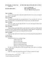
FIG. I. Title page of the 1619 edition of Napier'sMirifici logarithmornm
canonis descriptio. which also contains his Constrnctio,

excellent help in astronomy, viz. the logarithms: but. my lord. being by you
found out. 1 wonder nobody found it out before, when now known it is so
easy.I

</div>
(26)<div class='page_container' data-page=26>

RECOGNITION 13

they finally decided on log 10= I= 10°. In modem phrasing this
amounts to saying that if a positive numberN is written asN= IOL ,

thenL is the Briggsian or "common"logarithm ofN, written log,aN
or simply log N. Thus was born the concept of base.2

Napier readily agreed to these suggestions, but by then he was
already advanced in years and lacked the energy to compute a new set
of tables. Briggs undertook this task, publishing his results in 1624
under the title Arithmetica logarithmica. His tables gave the 
loga-rithms to base 10 of all integers from I to 20,000 and from 90,000 to
100,000 to an accuracy of fourteen decimal places. The gap from

20,000 to 90,000 was later filled by Adriaan Vlacq (1600-1667), a
Dutch publisher, and his additions were included in the second
edi-tion of the Arithmetica logarithmica (1628). With minor revisions,
this work remained the basis for all subsequent logarithmic tables up
to our century. Not until 1924 did work on a new set of tables,
accu-rate to twenty places, begin in England as part of the tercentenary
celebrations of the invention of logarithms. This work was completed
in 1949.

Napier made other contributions to mathematics as well. He
in-vented the rods or "bones" named after him-a mechanical device for
performing multiplication and division-and devised a set of rules
known as the "Napier analogies" for use in spherical trigonometry.
And he advocated the use of the decimal point to separate the whole
part of a number from its fractional part, a notation that greatly
sim-plified the writing of decimal fractions. None of these
accomplish-ments, however, compares in significance to his invention of
loga-rithms. At the celebrations commemorating the three-hundredth
anniversary of the occasion, held in Edinburgh in 1914, Lord
Moul-ton paid him tribute: "The invention of logarithms came on the world
as a bolt from the blue. No previous work had led up to it,
foreshad-owed it or heralded its arrival. It stands isolated, breaking in upon
human thought abruptly without borrowing from the work of other
intellects or following known lines of mathematical thought."3
Napier died at his estate on 3 April 1617 at the age of sixty-seven and
was buried at the church of St. Cuthbert in Edinburgh.4

Henry Briggs moved on to become, in 1619, the first Savilian
Pro-fessor of Geometry at Oxford University, inaugurating a line of
dis-tinguished British scientists who would hold this chair, among them

John Wallis, Edmond Halley, and Christopher Wren. At the same
time, he kept his earlier position at Gresham College, occupying the
chair that had been founded in 1596 by Sir Thomas Gresham, the
earliest professorship of mathematics in England. He held both
posi-tions until his death in 1631.

</div>
(27)<div class='page_container' data-page=27>

14 CHAPTER 2

a table of logarithms on the same general scheme as Napier's, but
with one significant difference: whereas Napier had used the
com-mon ratio I - 10-7, which is slightly less than I, BUrgi used I

+

10-4,
a number slightly greater than I. Hence BUrgi's logarithmsincrease

with increasing numbers, while Napier's decrease. Like Napier,
BUrgi was overly concerned with avoiding decimal fractions, making
his definition of logarithms more complicated than necessary. If a
positive integerNis written asN= I08( I +10-4)L, then BUrgi called
the number 10L (rather thanL)the "red number" corresponding to the
"black number" N. (In his table these numbers were actually printed
in red and black, hence the nomenclature.) He placed the red
num-bers-that is, the logarithms-in the margin and the black numbers
in the body of the page, in essence constructing a table of
"antiloga-rithms." There is evidence that BUrgi arrived at his invention as early
as 1588, six years before Napier began work on the same idea, but for
some reason he did not publish it until 1620, when his table was
issued anonymously in Prague. In academic matters the iron rule is
"publish or perish." By delaying publication, BUrgi lost his claim for
priority in a historic discovery. Today his name, except among
histo-rians of science, is almost forgotten. s

The use of logarithms quickly spread throughout Europe. Napier's

Descriptio was translated into English by Edward Wright (ca.

1560-1615, an English mathematician and instrument maker) and appeared
in London in 1616. Briggs's and Vlacq's tables of common
loga-rithms were published in Holland in 1628. The mathematician
Bona-ventura Cavalieri (1598-1647), a contemporary ofGalileo and one of
the forerunners of the calculus, promoted the use of logarithms in
Italy, as did Johannes Kepler in Germany. Interestingly enough, the
next country to embrace the new invention was China, where in 1653
there appeared a treatise on logarithms by Xue Fengzuo, a disciple of
the Polish Jesuit John Nicholas Smogule~ki(1611-1656). Vlacq's
tables were reprinted in Beijing in 1713 in the Lu-Li Yuan Yuan

(Ocean of calendar calculations). A later work, Shu Li Ching Yun

(Collected basic principles of mathematics), was published in Beijing
in 1722 and eventually reached Japan. All of this acti vity was a result
of the Jesuits' presence in China and their commitment to the spread
of Western science.6

</div>
(28)<div class='page_container' data-page=28>

RECOGNITION 15

measured and then added or subtracted with a pair of dividers. The
idea of using two logarithmic scales that can be moved along each
other originated with William Oughtred (1574-1660), who, like
Gunter, was both a clergyman and a mathematician. Oughtred seems
to have invented his device as early as 1622, but a description was not
published until ten years later. In fact, Oughtred constructed two

ver-sions: a linear slide rule and a circular one, where the two scales were
marked on discs that could rotate about a common pivot.?

Though Oughtred held no official university position, his
contribu-tions to mathematics were substantial. In his most influential work,
the Cia vis mathematicae (1631), a book on arithmetic and algebra, he
introduced many new mathematical symbols, some of which are still
in use today. (Among them is the symbol

x

for multiplication, to
which Leibniz later objected because of its similarity to the letterx;
two other symbols that can still be seen occasionally are: : to denote
a proportion and ~ for "the difference between.") Today we take for
granted the numerous symbols that appear in the mathematical
litera-ture, but each has a history of its own, often reflecting the state of
mathematics at the time. Symbols were sometimes invented at the
whim of a mathematician; but more often they were the result of a
slow evolution, and Oughtred was a major player in this process.
Another mathematician who did much to improve mathematical
no-tation was Leonhard Euler, who will figure prominently later in our
story.

About Oughtred's life there are many stories. As a student at
King's College in Cambridge he spent day and night on his studies,
as we know from his own account: "The time which over and above
those usuall studies I employed upon the Mathematicall sciences, I
redeemed night by night from my naturall sleep, defrauding my body,
and inuring it to watching, cold, and labour, while most others tooke
their rest."8 We also have the colorful account of Oughtred in John
Aubrey's entertaining (though not always reliable) Brief Lives:

He was a little man, had black haire, and blacke eies (with a great deal of

spirit). His head was always working. He would drawe lines and diagrams on
the dust ... did use to lye a bed tiII eleaven or twelve a clock.... Studyed
late at night; went not to bed till II a clock; had his tinder box by him;
and on the top of his bed-staffe, he had his inke-home fix't. He slept but little.
Sometimes he went not to bed in two or three nights.9

Though he seems to have violated every principle of good health,
Oughtred died at the age of eighty-six, reportedly ofjoy upon hearing
that King Charles II had been restored to the throne.

</div>
(29)<div class='page_container' data-page=29>

Mathemati-16 CHAPTER 2

call Ring, in which he described a circular slide rule he had invented.

In the preface, addressed to King Charles I (to whom he sent a slide
rule and a copy of the book), Delamain mentions the ease of
opera-tion of his device, noting that it was "fit for use ... as well on Horse
backe as on Foot."l0 He duly patented his invention, believing that
his copyright and his name in history would thereby be secured.
However, another pupil of Oughtred, William Forster, claimed that
he had seen Oughtred's slide rule at Delamain's home some years
earlier, implying that Delamain had stolen the idea from Oughtred.
The ensuing series of charges and countercharges was to be expected,
for nothing can be more damaging to a scientist's reputation than an
accusation of plagiarism. It is now accepted that Oughtred was
in-deed the inventor of the slide rule, but there is no evidence to support
Forster's claim that Delamain stole the invention. In any event, the
dispute has long since been forgotten, for it was soon overshadowed
by a far more acrimonious dispute over an invention of far greater
importance: the calculus.

The slide rule, in its many variants, would be the faithful
compan-ion of every scientist and engineer for the next 350 years, proudly
given by parents to their sons and daughters upon graduation from
college. Then in the early 1970s the first electronic hand-held
calcu-lators appeared on the market, and within ten years the slide rule was
obsolete. (In 1980 a leading American manufacturer of scientific
in-struments, Keuffel& Esser, ceased production of its slide rules, for
which it had been famous since 1891.11 ) As for logarithmic tables,
they have fared a little better: one can still find them at the back of
algebra textbooks, a mute reminder of a tool that has outlived its
usefulness.Itwon't be long, however, before they too will be a thing
of the past.

But if logarithms have lost their role as the centerpiece of
computa-tional mathematics, the logarithmicfunction remains central to

al-most every branch of mathematics, pure or applied. Itshows up in a
host of applications, ranging from physics and chemistry to biology,
psychology, art, and music. Indeed, one contemporary artist, M. C.
Escher, has made the the logarithmic function-disguised as a
spi-ral-a central theme of much of his work (see p. 138).

In the second edition of Edward Wright's translation of Napier's

De-scriptio (London, 1618), in an appendix probably written by

</div>
(30)<div class='page_container' data-page=30>

RECOGNITION 17

from? Wherein lies its importance? To answer these questions, we

must now tum to a subject that at first seems far removed from
expo-nents and logarithms: the mathematics of finance.

NOTES AND SOURCES

I. Quoted in Eric Temple Bell, Men of Mathematics (1937; rpt. 
Har-mondsworth: Penguin Books, 1965),2:580; Edward Kasner and James
New-man, Mathematics and the Imagination (New York: Simon and Schuster,
1958), p. 81. The original appears in Lilly's Description ofhis Life and Times
(1715).

2. See George A. Gibson, "Napier's Logarithms and the Change to
Briggs's Logarithms," in Napier Tercentenary Memorial Volume, ed. Cargill
Gilston Knott (London: Longmans, Green and Company, 1915), p. III. See
also Julian Lowell Coolidge, The Mathematics of Great Amateurs (New
York: Dover, 1963), ch. 6, esp. pp. 77-79.

3. Inaugural address, "The Invention of Logarithms," in Napier

Tercen-tenary Memorial Volume, p. 3.

4. Handbook ofthe Napier Tercentenary Celebration, or Modern 
Instru-ments and Methods of Calculation, ed. E. M. Horsburgh (1914; Los Angeles:

Tomash Publishers, 1982), p. 16. Section A is a detailed account of Napier's
life and work.

5. On the question of priority, see Florian Cajori, "Algebra in Napier's
Day and Alleged Prior Inventions of Logarithms," in Napier Tercente:lary

Memorial Volume, p. 93.

6. Joseph Needham, Science and Civilisation in China (Cambridge:
Cambridge University Press, 1959), 3:52-53.

7. David Eugene Smith, A Source Book in Mathematics (1929; rpt. New
York: Dover, 1959), pp. 160-164.

8. Quoted in David Eugene Smith, History of Mathematics, 2 vols.
(1923; New York: Dover, 1958), 1:393.

9. John Aubrey, Brief Lives, 2: 106 (as quoted by Smith, History of

Math-ematics, 1:393).

10. Quoted in Smith, A Source Book in Mathematics, pp. 156-159.
II. New York Times, 3 January 1982.

</div>
(31)<div class='page_container' data-page=31>

Computing with Logarithms

F o r many of us-at least those who completed our college education
after 1980-10garithms are a theoretical subject, taught in an
intro-ductory algebra course as part of the function concept. But until the
late 1970s logarithms were still widely used as a computational
de-vice, virtually unchanged from Briggs's common logarithms of 1624.
The advent of the hand-held calculator has made their use obsolete.

Let us say it is the year 1970 and we are asked to compute the
ex-pression

x= 3~(493.8.23.672/5.104).

For this task we need a table of four-place common logarithms
(which can still be found at the back of most algebra textbooks). We
also need to use the laws of logarithms:

log (ab)

=

log a

+

log b, log (alb)

=

log a -log b,
log a"=n log a,

whereaand b denote any positive numbers andnany real number;
here "log" stands for common logarithm-that is, logarithm base
IO-although any other base for which tables are available could be
used.

Before we start the computation, let us recall the definition of
loga-rithm: If a positive number N is written as N= IOL , then L is the
logarithm (base 10) ofN, written log N. Thus the equationsN= IQL
and L =logN are equivalent-they give exactly the same
informa-tion. Since I

=

100 and 10

=

10', we have log I

=

0 and log 10

=

1.
Therefore, the logarithm of any number between I (inclusive) and
10 (exclusive) is a positive fraction, that is, a number of the form

o.

abc . .. ;in the same way, the logarithm of any number between
10 (inclusive) and 100 (exclusive) is of the form I . abc . .. , and so
on. We summarize this as:

Range ofN 10gN

</div>
(32)<div class='page_container' data-page=32>

COMPUTING WITH LOGARITHMS 19

(The table can be extended backward to include fractions, but we
have not done so here in order to keep the discussion simple.) Thus,
if a logarithm is written as log N=p .abc . .. ,the integerp tells us
in what range of powers of lathe numberN lies; for example, if we
are told that log N =3.456, we can conclude that N lies between
1,000 and 10,000. The actual value ofN is determined by the
frac-tional part. abc . .. of the logarithm. The integral partp of log N is
called its characteristic, and the fractional part. abc . .. its

man-tissa.1A table of logarithms usually gives only the mantissa; it is up

to the user to determine the characteristic. Note that two logarithms
with the same mantissa but different characteristics correspond to
two numbers having the same digits but a different position of the
decimal point. For example, logN=0.267 corresponds toN= 1.849,
whereas logN

=

1.267 corresponds toN

=

18.49. This becomes clear
if we write these two statements in exponential form: 10° 267= 1.849,
while 101.267

=

10· 10°·267

=

10· 1.849

=

18.49.

We are now ready to start our computation. We begin by writingx
in a form more suitable for logarithmic computation by replacing the
radical with a fractional exponent:

x =(493.8.23.672/5.104)1/3.

Taking the logarithm of both sides, we have

logx=(1/3)[log 493.8

+

2 log 23.67 - log 5.104].

We now find each logarithm, using the Proportional Parts section of

the table to add the value given there to that given in the main table.
Thus, to find log 493.8 we locate the row that starts with 49, move
across to the column headed by 3 (where we find 6928), and then look
under the column 8 in the Proportional Parts to find the entry 7. We
add this entry to 6928 and get 6935. Since 493.8 is between 100 and
1,000, the characteristic is 2; we thus have log 493.8=2.6935. We do
the same for the other numbers.Itis convenient to do the computation
in a table:

N 10gN

23.67 -7 1.3742

x 2

2.7484
493.8 -7 +2.6935
5.4419
5.104 -7 - 0.7079

</div>
(33)<div class='page_container' data-page=33>

20 COMPUTING WITH LOGARITHMS

N 0 1 2 3 4 5 6 7 8 9 Proportional Parts

1 2 3 4 5 6 7 8 9

10 0000 0043 0086 0128 0170 0212 0253 0294 0334 0374 4 8 12 17 21 25 29 33 37
11 0414 0453 0492 0531 0569 0607 0645 0682 0719 0755 4 8 11 15 19 23 26 30 34
12 0792 0828 0864 0899 0934 0969 1004 1038 1072 1106 3 7 10 14 17 21 24 28 31
13 1139 1173 1206 1239 1271 1303 1335 1367 1399 1430 3 6 10 13 16 19 23 26 29

14 1461 1492 1523 1553 1584 1614 1644 1673 1703 1732 3 6 9 12 15 18 21 24 27
15 1761 1790 1818 1847 1875 1903 1931 1959 1987 2014 3 6 8 11 14 17 20 22 25
16 2041 2068 2095 2122 2148 2175 2201 2227 2253 2279 3 5 8 11 13 16 18 21 24
17 2304 2330 2355 2380 2405 2430 2455 2480 2504 2529 2 5 7 10 12 15 17 20 22
18 2553 2577 2601 2625 2648 2672 2695 2718 2742 2765 2 5 7 9 12 14 16 19 21
19 2788 2810 2833 2856 2878 2900 2923 2945 2967 2989 2 4 7 9 11 13 16 18 20
20 3010 3032 3054 3075 3096 3118 3139 3160 3181 3201 2 4 6 8 11 13 15 17 19
21 3222 3243 8263 8284 3304 3324 3345 336& 3385 3404 2 4 6 8 10 12 14 16 18
22 3424 8444 3464 3483 3502 352~560 3579 3598 2 4 6 8 10

W

5 17

23 3617 3636 3655 3674 3692 371 3729 747 3766 3784 2 4 6 7 9 13 5 17
24 3802 3820 3838 3856 3874 389 39 3927 3945 3962 2 4 5 7 9 1 4 16
25 3979 3997 4014 4031 4048 4065 4082 4099 4116 4133 2 3 5 7 9 10 12 14 15
26 4150 4166 4183 4200 4216 4232 4249 4265 4281 4298 2 3 5 7 8 10 11 13 15
27 4314 4330 4346 4362 4378 4393 4409 4425 4440 4456 2 3 5 6 8 9 11 13 14
28 4472 4487 4502 4518 4533 4548 4564 4579 4594 4609 2 3 5 6 8 9 11 12 14
29 4624 4639 4654 4669 4683 4698 4713 4728 4742 4757 1 3 4 6 7 9 10 12 13
30 4771 4786 4800 4814 4829 4843 4857 4871 4886 4900 1 3 4 6 7 9 10 11 13
31 4914 4928 4942 4955 4969 4983 4997 5011 5024 5038 1 3 4 6 7 8 10 11 12
32 5051 5065 5079 5092 5105 5119 5132 5145 5159 5172 1 3 4 5 7 8 9 11 12
33 5185 5198 5211 5224 5237 5250 5263 5276 5289 5302 1 3 4 5 6 8 9 10 12
34 5315 5328 5340 5353 5366 5378 5391 5403 5416 5428 1 3 4 5 6 8 9 10 11
35 5441 5453 5465 5478 5490 5502 5514 5527 5539 5551 1 2 4 5 6 7 9 10 11
36 5563 5575 5587 5599 5611 5623 5635 5647 5658 5670 1 2 4 5 6 7 8 10 11
37 5682 5694 5705 5717 5729 5740 5752 5763 5775 5786 1 2 3 5 6 7 8 9 10
38 5798 5809 5821 5832 5848 5855 5866 5877 5888 5899 1 2 3 5 6 7 8 9 10
39 5911 5922 5933 5944 5955 5966 5977 5988 5999 6010 1 2 3 4 5 7 8 9 10
40 6021 6031 6042 6053 6064 6075 6085 6096 6107 6117 1 2 3 4 5 6 8 9 10

41 6128 6138 6149 6160 6170 6180 6191 6201 6212 6222 1 2 3 4 5 6 7 8 9
42 6232 6243 6253 6263 6274 6284 6294 6304 6314 6325 1 2 3 4 5 6 7 8 9
43 6335 6345 6355 6365 6375 6385 6395 6405 6415 6425 1 2 3 4 5 6 7 8 9
44 6435 6444 6454 6464 6474 6484 6493 6503 6513 6522 1 2 3 4 5 6 7 8 9
45 6532 6542 6551 6561 6571 6580 6590 6599 6609 6618 1 2 3 4 5 6 7 8 9
46 6628 6637 6646 6656 6665 6675 6684 6693 6702 6712 1 2 3 4 5 6 7 7 8
47 6721 6730 6739 6749 6758 6767 6776 6785 6794 6803 1 2 3 4 5 5 6 7 8
48 6812 6821 683~848 6857 6866 6875 6884 6893 1 2 3 4 4 5

rQ

49 6902 6911 692 6928 937 6946 6955 6964 6972 6981 1 2 3 4 4 5
50

~~8

7007 6 7024 7033 7042 7050 7059 7067 1 2

m

51 7076 084 7093 7101 7110 7118 7126 7135 7143 7152 1 2 5 6 7 8
52 7 7168 7177 7185 7193 7202 7210 7218 7226 7235 1 2 5 6 7 7
53 7243 7251 7259 7267 7275 7284 7292 7300 7308 7316 1 2 2 3 4 5 6 6 7
54 7324 7332 7340 7348 7356 7364 7372 7380 7388 7396 1 2 2 3 4 5 6 6 7

N 0 1 2 3 4 5 6 7 8 9 1 2 3 4 5 6 7 8 9

Four-Place Logarithms

</div>
(34)<div class='page_container' data-page=34>

COMPUTING WITH LOGARITHMS 21

p 0 1 2 3 4 5 6 7 8 9 1 2 Proportional Parts

3 4 5 6 7 8 9
.50 3162 3170 3177 3184 3192 3199 3206 3214 3221 3228 1 1 2 3 4 4 5 6 7
.61 3236 3243 3261 3268 3266 3273 3281 3289 3296 3304 1 2 2 3 4 6 6 6 7
.62 3311 3319 3327 3334 3342 3360 3367 3366 3373 3381 1 2 2 3 4 6 6 6 7
.63 3388 3396 3404 3412 3420 3428 3436 3443 3461 3469 1 2 2 3 4 6 6 6 7
.54 3467 3476 3483 3491 3499 3508 3616 3624 3632 3640 1 2 2 3 4 5 6 6 7
.66 3648 3666 3666 3573 3581 3689 3597 3606 3614 3622 1 2 2 3 4 6 6 7 7
.56 3631 3639 3648 3656 3664 3673 3681 369~707 1 2 3 3 4 5 6 7 8
.57 3715 3724 3733 3741 3750 3758 3767 377 3784 793 1 2 3 3 4 5 6 7 8
.58 3802 3811 3819 3828 3837 3846 3856 386 3882 1 2 3 4 4 5 6 7 8
.59 3890 3899 3908 3917 3926 3936 3945 3954 3963 3972 1 2 3 4 6 5 6 7 8
.60 3981 3990 3999 4009 4018 4027 4036 4046 4055 4064 1 2 3 4 5 6 6 7 8
.61 4074 4083 4093 4102 4111 4121 4130 4140 4150 4159 1 2 3 4 5 6 7 8 9
.62 4169 4178 4188 4198 4207 4217 4227 4236 4246 4256 1 2 3 4 5 6 7 8 9
.63 4266 4276 4285 4295 4305 4315 4326 4335 4345 4355 1 2 3 4 5 6 7 8 9
.64 4365 4375 4385 4395 4406 4416 4426 4436 4446 4457 1 2 3 4 5 6 7 8 9
.65 4467 4477 4487 4498 4508 4519 4529 4539 4550 4560 1 2 3 4 5 6 7 8 9
.66 4571 4581 4592 4603 4613 4624 4634 4645 4656 4667 1 2 3 4 5 6 7 9 10
.67 4677 4688 4699 4710 4721 4732 4742 4753 4764 4775 1 2 3 4 5 7 8 9 10
.68 4786 4797 4808 4819 4831 4842 4853 4864 4875 4887 1 2 3 4 6 7 8 9 10
.69 4898 4909 4920 4932 4943 4965 4966 4977 4989 5000 1 2 3 5 6 7 8 9 10
.70 6012 5023 5035 5047 5058 5070 5082 5093 5105 5117 1 2 4 5 6 7 8 9 11
.71 5129 5140 5152 5164 5176 5188 5200 5212 5224 5236 1 2 4 6 6 7 8 10 11
.72 5248 5260 5272 6284 5297 5309 6321 5333 5346 5358 1 2 4 5 6 7 9 10 11
.73 5370 5383 5395 5408 6420 5433 5445 5458 5470 5483 1 3 4 5 6 8 9 10 11
.74 5496 5508 5521 5534 5546 5559 5572 5585 5698 5610 1 3 4 5 6 8 9 10 12
.75 6623 5636 5649 6662 5675 5689 5702 5716 5728 5741 1 3 4 5 7 8 9 10 12
.76 5754 5768 5781 5794 5808 5821 5834 5848 6861 5875 1 3 4 5 7 8 9 11 12
.77 5888 5902 5916 5929 5943 5957 5970 5984 5998 6012 1 3 4 5 7 8 10 11 12

.78 6026 6039 6063 6067 6081 6095 6109 6124 6138 6152 1 3 4 6 7 8 10 11 13
.79 6166 6180 6194 6209 6223 6237 6252 6266 6281 6295 1 3 4 6 7 9 10 11 13
.80 6310 6324 6339 6353 6368 6383 6397 6412 6427 6442 1 3 4 6 7 9 10 12 13
.81 6457 6471 6486 6501 6616 6531 6546 6561 6577 6592 2 3 5 6 8 9 11 12 14
.82 6607 6622 6637 6653 6668 6683 6699 6714 6730 6745 2 3 5 6 8 9 11 12 14
.83 6761 6776 6792 6808 6823 6839 6855 6871 6887 6902 2 3 5 6 8 9 11 13 14
.84 6918 6934 6950 6966 6982 6998 7016 7031 7047 7063 2 3 5 6 8 10 11 13 15
.85 7079 7096 7112 7129 7145 7161 7178 7194 7211 7228 2 3 5 7 8 10 12 13 15

.86 7244 7261 7278 7296 7311 7328 7346 7362 7379 7396 2 3 5 7 8 10 12 13 15
.87 7413 7430 7447 7464 7482 7499 7516 7534 7551 7568 2 3 6 7 9 10 12 14 16
.88 7586 7603 7621 7638 7656 7674 7691 7709 7727 7745 2 4 5 7 9 11 12 14 16
.89 7762 7780 7798 7816 7834 7852 7870 7889 7907 7925 2 4 5 7 9 11 13 14 16
.90 7943 7962 7980 7998 8017 8035 8054 8072 8091 8110 2 4 6 7 9 11 13 16 17
.91 8128 8147 8166 8185 8204 8222 8241 8260 8279 8299 2 4 6 8 9 11 13 15 17
.92 8318 8337 8356 8375 8395 8414 8433 8453 8472 8492 2 4 6 8 10 12 14 15 ta
.93 8611 8531 8551 8570 8590 8610 8630 8650 8670 8690 2 4 6 8 10 12 14 16 18
.94 8710 8730 8750 8770 8790 8810 8831 8851 8872 8892 2 4 6 8 10 12 14 16 18
.95 8913 8933 8954 8974 8995 9016 9036 9057 9078 9099 2 4 6 8 10 12 15 17 19
.96 9120 9141 9162 9183 9204 9226 9247 9268 9290 9311 2 4 6 8 11 13 15 17 19
.97 9333 9354 9376 9397 9419 9441 9462 9484 9506 9528 2 4 7 9 11 13 15 17 20
.98 9550 9572 9594 9616 9638 9661 9683 9705 9727 9750 2 4 7 9 11 13 16 18 20
.99 9772 9795 9817 9840 9863 9886 9908 9931 9964 9977 2 5 7 9 11 14 16 18 20

P 0 1 2 3 4 5 6 7 8 9 1 2 3 4 5 6 7 8 9

Four-Place Antilogarithms

</div>
(35)<div class='page_container' data-page=35>

22 COMPUTING WITH LOGARITHMS

were invented, to around 1945, when the first electronic computers
became operative, logarithms-or their mechanical equivalent, the
slide rule-were practically the only way to perform such
calcula-tions. No wonder the scientific community embraced them with such
enthusiasm. As the eminent mathematician Pierre Simon Laplace
said, "By shortening the labors, the invention of logarithms doubled
the life of the astronomer."

NOTE

</div>
(36)<div class='page_container' data-page=36>

3 Financial Matters

If thou lend money to any of My people. ...

thou shalt not be to him as a creditor;

neither shall ye lay upon him interest.

-EXODUS22:24

From time immemorial money matters have been at the center of
human concerns. No other aspect of life has a more mundane
charac-ter than the urge to acquire wealth and achieve financial security. So
it must have been with some surprise that an anonymous
mathema-tician-or perhaps a merchant or moneylender-in the early
seven-teenth century noticed a curious connection between the way money
grows and the behavior of a certain mathematical expression at
infinity.

Central to any consideration of money is the concept of interest, or
money paid on a loan. The practice of charging a fee for borrowing
money goes back to the dawn of recorded history; indeed, much of
the earliest mathematical literature known to us deals with questions
related to interest. For example, a clay tablet from Mesopotamia,
dated to about 1700H.C.and now in the Louvre, poses the following
problem: How long will it take for a sum of money to double if
in-vested at 20 percent interest rate compounded annually?' To
formu-late this problem in the language of algebra, we note that at the end
of each year the sum grows by 20 percent, that is, by a factor of 1.2;
hence afterxyears the sum will grow by a factor of 1.2x

•Since this is

to be equal to twice the original sum, we have 1.2x =2 (note that the

original sum does not enter the equation).

</div>
(37)<div class='page_container' data-page=37>

24 CHAPTER 3

2.0736. This leads to a linear (first-degree) equation inx, which can
easily be solved using elementary algebra. But the Babylonians did
not possess our modem algebraic techniques, and to find the required
value was no simple task for them. Still, their answer, x=3.7870,
comes remarkably close to the correct value, 3.8018 (that is, about
three years, nine months, and eighteen days). We should note that the
Babylonians did not use our decimal system, which came into use
only in the early Middle Ages; they used the sexagesimal system, a
numeration system based on the number 60. The answer on the

Louvre tablet is given as 3;47,13,20, which in the sexagesimal
sys-tem means 3

+

47/60

+

13/602

+

20/603,or very nearly 3.7870.2

In a way, the Babylonians did use a logarithmic table of sorts.
Among the surviving clay tablets, some list the first ten powers of the
numbers 1/36, 1/16, 9, and 16 (the first two expressed in the
sexa-gesimal system as 0; 1,40 and 0;3,45)-all perfect squares. Inasmuch
as such a table lists the powers of a number rather than the exponent,
it is really a table of antilogarithms, except that the Babylonians did
not use a single, standard base for their powers. It seems that these
tables were compiled to deal with a specific problem involving
com-pound interest rather than for general use.3

Let us briefly examine how compound interest works. Suppose we
invest $100 (the "principal") in an account that pays 5 percent
in-terest, compounded annually. At the end of one year, our balance will
be 100 x 1.05=$105. The bank will then consider this new amount
as a new principal that has just been reinvested at the same rate. At
the end of the second year the balance will therefore be 105 x
1.05=$110.25, at the end of the third year 110.25 x 1.05=$115.76,
and so on. (Thus, not only the principal bears annual interest but also
the interest on the principal-hence the phrase "compound interest.")
We see that our balance grows in a geometric progression with the
common ratio 1.05. By contrast, in an account that pays simple 
inter-est the annual rate is applied to the original principal and is therefore
the same every year. Had we invested our $100 at 5 percent simple
interest, our balance would increase each year by $5, giving us the
arithmetic progression 100, 105, 110,115, and so on. Clearly, money
invested at compound interest-regardless of the rate-will
eventu-ally grow faster than if invested at simple interest.

</div>
(38)<div class='page_container' data-page=38>

FINANCIAL MATTERS

S= P(1 +r)/.

25

(1)

This formula is the basis of virtually all financial calculations,
whether they apply to bank accounts, loans, mortgages, or annuities.
Some banks compute the accrued interest not once but several
times a year. If, for example, an annual interest rate of 5 percent is
compounded semiannually, the bank will use one-half of the annual
interest rate as the rate per period. Hence, in one year a principal of
$100 will be compounded twice, each time at the rate of 2.5
per-cent; this will amount to 100 x 1.0252or $ I05.0625, about six cents
more than the same principal would yield if compounded annually at
5 percent.

In the banking industry one finds all kinds of compounding

schemes-annual, semiannual, quarterly, weekly, and even daily.
Suppose the compounding is done n times a year. For each 
"conver-sion period" the bank uses the annual interest rate divided by n, that
is, r/n. Since in t years there are (nt) conversion periods, a principal
Pwill aftertyears yield the amount

PO

+

r/n)n/.

(2)

Of course, equation I is just a special case of equation 2-the case
where n= I.

Itwould be interesting to compare the amounts of money a given
principal will yield after one year for different conversion periods,
assuming the same annual interest rate. Let us take as an example
P

=

$100 and r

=

5 percent

=

0.05. Here a hand-held calculator will
be useful. Ifthe calculator has an exponentiation key (usually
de-noted byy(), we can use it to compute the desired values directly;
otherwise we will have to use repeated multiplication by the factor
(I +0.05/n).The results, shown in table 3. I, are quite surprising. As
we see, a principal of $ 100 compounded daily yields just thirteen
cents more than when compounded annually, and about one cent

TABLE3.1. $I00 Invested for One Year at 5 Percent
Annual Interest Rate at Different Conversion Periods

</div>
(39)<div class='page_container' data-page=39>

26 CHAPTER 3

more than when compounded monthly or weekly! Ithardly makes a
difference in which account we invest our money.4

To explore this question further, let us consider a special case of
equation 2, the case when r= 1. This means an annual interest rate of
100 percent, and certainly no bank has ever come up with such a
generous offer. What we have in mind, however, is not an actual
situation but a hypothetical case, one that has far-reaching
mathe-matical consequences. To simplify our discussion, let us assume that
P

=

$1 andt

=

1 year. Equation 2 then becomes

S=(l

+

l/n)n (3)

and our aim is to investigate the behavior of this formula for
increas-ing values ofn. The results are given in table 3.2.

TABLE3.2

n (I +I/n)n

I 2

2 2.25

3 2.37037

4 2.44141

5 2.48832

10 2.59374

50 2.69159

100 2.70481
1,000 2.71692
10,000 2.71815
100,000 2.71827
1,000,000 2.71828
10,000,000 2.71828

It looks as if any further increase in n will hardly affect the 
out-come-the changes will occur in less and less significant digits.

But will this pattern go on? Is it possible that no matter how large

</div>
(40)<div class='page_container' data-page=40>

FINANCIAL MA TTERS 27

sorts proliferated; as a result, a great deal of attention was paid to the
law of compound interest, and it is possible that the number e 
re-ceived its first recognition in this context. We shall soon see,
how-ever, that questions unrelated to compound interest also led to the
same number at about the same time. But before we tum to these
questions, we would do well to take a closer look at the mathematical
process that is at the root ofe: the limit process.

NOTES ANDSOURCES

I. Howard Eves, An Introduction to the History of Mathematics (1964;
rpt.Philadelphia: Saunders College Publishing, 1983), p. 36.

2. Carl B. Boyer, A History of Mathematics, rev. ed. (New York: John
Wiley, 1989), p. 36.

3. Ibid., p. 35.

</div>
(41)<div class='page_container' data-page=41>

4 To the

Limit~

If It Exists

I saw, as one might see the transit of Venus, a quantity

passing through infinity and changing its sign from plus to

minus. I saw exactly how it happened . .. but it was after

dinner and I let it go.

-SIR WINSTON CHURCHILL,My Early Life(1930)

At first thought, the peculiar behavior of the expression (l

+

lIn)n

for large values ofn must seem puzzling indeed. Suppose we

con-sider only the expression inside the parentheses, 1+ lin. As n

in-creases, lin gets closer and closer to 0 and so 1+ lingets closer and
closer to 1, although it will always be greater than 1.Thus we might
be tempted to conclude that for "really large" n (whatever "really
large" means), 1+lin, to every purpose and extent, may be

re-placed by 1. Now 1 raised to any power is always equal to 1, so it
seems that(l +lIn)n for large n should approach the number1.Had
this been the case, there would be nothing more for us to say about the
subject.

But suppose we follow a different approach. We know that when
a number greater than 1 is raised to increasing powers, the result
be-comes larger and larger. Since 1+lin is always greater than 1, we

might conclude that (1 + lIn)n, for large values of n, will grow

with-out bound, that is, tend to infinity. Again, that would be the end of our
story.

That this kind of reasoning is seriously flawed can already be seen
from the fact that, depending on our approach, we arrived at two
different results: 1 in the first case and infinity in the second.In

math-ematics, the end result of any valid numerical operation, regardless of
how it was arrived at, must always be the same. For example, we can
evaluate the expression 2 . (3+4) either by first adding 3 and 4 to get
7 and then doubling the result, or by first doubling each of the
num-bers 3 and 4 and then adding the results. In either case we get 14.

Why, then, did we get two different results for(l + lIn)n?

</div>
(42)<div class='page_container' data-page=42>

expres-TO THE LIMIT, IF IT EXISTS 29

sion 2 . (3+4) by the second method, we tacitly used one of the
fun-damentallaws of arithmetic, the distributive law, which says that for
any three numbersx,y, andzthe equationx .(y

+

z)=x .y

+

x .zis
always true. To go from the left side of this equation to the right side
is a valid operation. An example of an invalid operation is to write
;/(9+ 16)

=

3+4

=

7, a mistake that beginning algebra students
often make. The reason is that taking a square root is not a
distribu-tive operation; indeed, the only proper way of evaluating ;/(9

+

16) is

first to add the numbers under the radical sign and then take the
square root: ;/(9

+

16)=;/25=5. Our handling of the expression
(l

+

IIn)n was equally invalid, because we wrongly played with one
of the most fundamental concepts of mathematical analysis: the

con-cept of limit.

When we say that a sequence of numbers aI, az, a3, ... , an, ...

tends to a limitLasn tends to infinity, we mean that as n grows larger

and larger, the tenus of the sequence get closer and closer to the
num-berL.Put in different words, we can make the difference (in absolute
value) between an and L as small as we please by going out far
enough in our sequence-that is, by choosing n to be sufficiently
large. Take, for example, the sequence 1, 112, 113, 114, ... , whose
general tenu is an= lin. As n increases, the terms get closer and
closer to O. This means that the difference between lin and the limit

a

(that is, just lin) can be made as small as we please if we choose n
large enough. Say that we want lin to be less than 111,000; all we
need to do is make n greater than 1,000. If we want lin to be less than
111,000,000, we simply choose anyngreater than 1,000,000. And so
on. We express this situation by saying that lin tends to

a

as n 
in-creases without bound, and we write lin ~

a

as n~00. We also use

the abbreviated notation

lim

J-.

=O.

n400n

A word of caution is necessary, however: the expressionlimn---+~lIn=

a

says only that the limit of lin as n ~00 is 0; it does not say that

linitself will ever be equal to O--in fact, it will not. This is the very
essence of the limit concept: a sequence of numbers can approach a
limit as closely as we please, but it will never actually reach it.'

For the sequence lin, the outcome of the limiting process is quite
predictable. In many cases, however, it may not be immediately clear
what the limiting value will be or whether there is a limit at all. For
example, the sequence an=(2n

+

1)/(3n

+

4), whose tenus for n= 1,
2, 3, ... are 3/7,5/10,7113, ... , tends to the limit 2/3 as n ~00.This

can be seen by dividing the numerator and denominator by n, giving
us the equivalent expression an=(2

+

IIn)/(3

+

4In).As n ~00,both

</div>
(43)<div class='page_container' data-page=43>

30 CHAPTER 4

other hand, the sequencean

=

(2n2+1)/(3n+4), whose members are

3/7,9/10, 19/13, ... , grows without bound as n~00. This is

be-cause the term n2causes the numerator to grow at a faster rate than
the denominator. We express this fact by writing limn--+~an=00,

al-though strictly speaking the sequence does not have a limit. A
limit-if it exists-must be a definite real number, and infinity is not a real
number.

For centuries, mathematicians and philosophers have been
in-trigued by the concept of infinity. Is there a number greater than all
numbers? If so, just how large is such a "number"? Can we calculate

with it as we do with ordinary numbers? And on the small scale of
things, can we divide a quantity-say a number or a line
segment-again and segment-again into smaller quantities, or will we eventually reach an
indivisible part, a mathematical atom that cannot be further split?
Questions such as these troubled the philosophers of ancient Greece
more than two thousand years ago, and they still trouble us
today-witness the never ending search for the elementary particles, those
elusive building blocks from which all matter is believed to be
constructed.

That we cannot use the symbol for infinity,00,as an ordinary

num-ber should be clear from the examples given above. For instance, if
we put n=00 in the expression (2n+ 1)/(3n+4), we would get

(200

+

1)/(300

+

4). Now, a multiple of00 is still 00, and a number

added to00is still00,so we should get00/00.Had00been an ordinary

number, subject to the ordinary rules of arithmetic, this expression
would simply be equal to 1. But it is not equal to I; it is 2/3, as we
have seen. A similar situation arises when we try to "compute"

00 - 00. Itwould be tempting to say that since any number when

sub-tracted from itself gives 0, we should have00 - 00=O. That this may

be false can be seen from the expression lIx2 - [(cos x)/x]2, where
"cos" is the cosine function studied in trigonometry. Asx~0, each
of the two terms tends to infinity; yet, with the help of a little

trigo-nometry, it can be shown that the entire expression approaches the
limit 1.

Expressions such as 00/00 or00 - 00 are known as "indeterminate

forms." These expressions have no preassigned value; they can be
evaluated only through a limiting process. Loosely speaking, in every
indeterminate form there is a "struggle" between two quantities, one
tending to make the expression numerically large, the other tending
to make it numerically small. The final outcome depends on the
pre-cise limiting process involved. The indeterminate forms most
com-monly encountered in mathematics are 0/0, 00/00, O· 00, 00 - 00, 0°,

00°, and I~. Itis to the last form that(I + lIn)nbelongs.

</div>
(44)<div class='page_container' data-page=44>

TO THE LIMIT, IF IT EXISTS 31

Of course, we could use a computer or a calculator to compute the
expression for very large values ofn, say a million or a billion. But
such a computation can only suggest the limiting value. We have no
assurance that this value will indeed hold up for a still largern.This
state of affairs underscores a fundamental difference between
mathe-matics and the sciences that are based on experimental or
observa-tional evidence, such as physics and astronomy. In those sciences,
if a certain result-say a numerical relation between the temperature
of a given amount of gas and its pressure-is supported by a large
number of experiments, that result may then be regarded as a law of
nature.

A classic example is afforded by the universal law of gravitation,

discovered by Isaac Newton and enunciated in his great work,

Philos-ophiae naturalis principia mathematica (1687). The law says that

any two material bodies-be they the sun and a planet revolving
around it or two paperclips placed on the table-exert on each other
a gravitational force proportional to the product of their masses and
inversely proportional to the square of the distance between them
(more precisely, between their centers of mass). For more than two
centuries this law was one of the rock foundations of classical
phys-ics; every astronomical observation seemed to corroborate it, and it is
still the basis for calculating the orbits of planets and satellites.Itwas
only in 1916 that Newton's law of gravitation was replaced by a more
refined law, Einstein's general theory of relativity. (Einstein's law
differs from Newton's only for extremely large masses and speeds
close to the speed of light.) Yet there is no way that Newton's
law-or any other law of physics-ean be proved in the mathematical sense
of the word. A mathematical proof is a chain of logical deductions,
all stemming from a small number of initial assumptions ("axioms")
and subject to the strict rules of mathematical logic. Only such a
chain of deductions can establish the validity of a mathematical law,
a theorem. And unless this process has been satisfactorily carried out,
no relation-regardless of how often it may have been confirmed by
observation-is allowed to become a law. Itmay be given the status
of a hypothesis or a conjecture, and all kinds of tentative results may
be drawn from it, but no mathematician would ever base definitive
conclusions on it.

</div>
(45)<div class='page_container' data-page=45>

32 CHAPTER 4

A binomial is any expression consisting of the sum of two terms;
we may write such an expression asa

+

b.One of the first things we
learn in elementary algebra is how to find successive powers of a
binomial-how to expand the expression (a

+

b)nfor n=0, 1,2, ....
Let us list the results for the first few n's:

(a+b)O= 1

(a+b)1

=

a+b
(a+b)2= a2+2ab+b2
(a+b)3= a3+3a2b+3ab2+b3
(a+b)4=a4+4a3b+6a2b2+4ab3+b4

From these few examples it is easy to see the general pattern: the
ex pansion of (a

+

b)nconsists of n

+

1 terms, each of the form an-kbk,
wherek=0, 1, 2, ... , n. Hence, as we go from left to right the 
expo-nent of a decreases from n to 0 (we can write the last term as aObn),
while that ofbincreases from 0 ton.The coefficients of the various
terms, known as the binomial coefficients, form a triangular scheme:

4
2

3 3

6 4

This scheme is known as Pascal's triangle, after the French 
philoso-pher and mathematician Blaise Pascal (1623-1662), who used it in
his theory of probability (the scheme itself had been known much

earlier; see figs. 2, 3, and 4). In this triangle, each number is the sum
of the two numbers immediately to its left and right in the row above

the number. For example, the numbers in the fifth row, 1, 4, 6, 4, 1,
are obtained from those in the fourth row as follows:

1 3 3 I

/\/\/\/\

1 4 6 4 1

(Note that the coefficients are the same whether we start from left or
right.)

</div>
(46)<div class='page_container' data-page=46>

TO THE LIMIT, IF IT EXISTS

£ynlme",e

~l1"O %""'gc~(jnore

,

"nt>cr~~Iim!t a~rcr l\aunhta"~

l'

een'

I

!

nUltg I!!

orcltn

Guchtr'Jlmic: (montn 1\e

!

geln

\m

fragflncfcn

6t~rifftJ1

•

t3U110er1

I

lid)

l\1ae

forrl

tmno

6d)t"bi~l'~it

in

~er

WtllC!Jl

practical.'"

t:oUetn

geGI.1ucht

~n1)tI

Oee

g(c'9d)tn

fiirma(fi

noiber

in

t:ttit3fcher

n(\d)

in

rodlener

fPzach nic

gcozncPr.

t'lJrch pctl'nm

2!pianu

~"n ~~'Pfjnicf/ij

2ttlronomti

"

'u jl1golfiat

<l)rbil1a~

i.

J'iLi

I~erremge~.

"

.

FIG.2. Pascal's
triangle appears on
the title page of an
arithmetic workby

Petrus Apianus
(Ingolstadt, 1527).

33

(1)

n'

nCk= .

k!(n-k)!

</div>
(47)<div class='page_container' data-page=47>

34 CHAPTER 4

FIG.3. Pascal's triangle in a
Japanese work of 1781.

;~\M~M

erN\'''''

CM"~N

"0

01;"0

1;;~~ n':~lt';M 1'l';"::~ M~ i'i~

O'l:~;M 10 :1>'01'1 ,£)~r,n 't:te'O (I'r')l,~l1:C'III')';) ~t:':

1 ( 11l~rI'~tW:llll'>p) eM: O"\lt'i'M

'p,;n,

1 (JD'5r1Dllm:f)

&;;0_

:,J..N (1 ""~D';t>1"

"'D

t'71t M'~W .5 J:1

§

,::;:;c;::;.'ll (ll ~D11'1;P\l; "';1'",~1.N

- - 1 "j;t; =,;.,i"

s:"":l(5"':'1l5,J..~1l (5 'j\l;"""":l.".,'lll:'Pj ,..

>'C';

M~,e'n
4.:,J..':N4....':'1l6..J-:·'1l4....4N(4 .:4N01' :l~'!:';1j\e; 1 1m" .

5:-:-...."':"'4:-N"';'5-.J..;:-'5:'lllO,J..':'lllO.J..:4115.J.."N (5 OP!:~ .,,~ '''~'P:~

oj"

1 ' ; . , . , ; . , . , , , 5 t"':"1
, CPPj OtP\ltp; \l" ODI;1;.,N.,.," 4~':l'
6:...~:1l6.J..·:'1l15... 3:511:10.J..':41115.J..:3116,J..611 (6 C'.,,'7I;e\le""." ")f'JDtlttm.,i"., .,iOMm

'71'~D;~;'711' ,." Il"~';;" .,~.""iP,;,,~~

FIG.4. The expansion of(a+b)"forn= I. 2. 3, ... , 6. From a Hebrew algebra book
by Hayim Selig Sionimski (Vilnius, 1834). The formulas use Hebrew letters and are
read from right to left.

The binomial formula can easily be proved for all positive integral
values ofn by the process known as mathematical induction: we

show that if the formula is true for all values of n up to, say, m, then
it must also be true for n

=

m

+

I (it is, of course, true for n

=

I, since

</div>
(48)<div class='page_container' data-page=48>

TO THE LIMIT, IF IT EXISTS 35

end after exactlyn+ I terms. As we shall see in Chapter 8, one of the
first great achievements of Isaac Newton was to extend this fonnula
to the case wheren is a negative integer or even a fraction; in these
cases the expansion will involve an infinite number of tenns.

A quick look at equation I will show that we can write it in an
alternative form,

lie _

n· (n - I) .(n - 2) ... (n - k

+

k - k!

(2)

This is because n! = I ·2·3· .... n while (n - k)!= I ·2·3· ....

(n - k), so that all the factors from I to (n - k) in the numerator of
equation I cancel with those in the denominator, leaving only the
factors n· (n - 1) .(n - 2)· .... (n - k+ I). With equation 2 in

mind, we can now apply the binomial fonnula to the expression
(l + IIn)ll. We have a = I and b = lin, so that

(

1+-

1)11

=I+n'-+

(I)

n· (n - I). -

(1)2

n n 2! n

n . (n - I) .(n - 2) .

(l)3

(l)11

+ 3! n + ... + l~

.

After a slight manipulation this becomes

( )

I I 2

lll_

(l-n) (l-n)·(I-n ) ~

I +n - I + I + 2! + 3! + ... + nil·

(3)

(4)

Since we are looking for the limit of (I + IIn)11 as n~00,we must let

n increase without bound. Our expansion will then have more and
more tenns. At the same time, the expression within each pair of
parentheses will tend to I, because the limits of lin, 21n, ... as n~00

are all O. We thus get

.

~

1)11

I I

hml+-

=1+1+-2,+-3'+ ....

11---7<'>0 n . .

We should add that even this derivation is not entirely sufficient to
prove that the desired limit does indeed exist (a complete proof is
found in Appendix 2). But for now let us accept the existence of this
limit as a fact. Denoting the limit by the letter e (more about the
choice of this letter later), we thus have

(5)

Not only is it much easier to compute the tenns of this infinite

</div>
(49)<div class='page_container' data-page=49>

36 CHAPTER 4

2= 2

2+ 1/2= 2.5

+

1/2

+

1/6= 2.666 ...

+

1/2

+

1/6

+

1/24= 2.708333 .

+

1/2

+

1/6

+

1/24

+

1/120= 2.716666 .

+

1/2

+

1/6

+

1/24

+

1/120

+

1/720= 2.7180555 .
2

+

1/2

+

1/6

+

1/24

+

1/120

+

1/720

+

1/5,040=2.718253968 .

We see that the terms of each sum decrease rapidly (this is because of
the rapid growth ofk! in the denominator of each term), so that the
series converges very fast. Moreover, since all terms are positive, the
convergence ismonotone:each additional term brings us closer to the
limit (this is not so with a series whose terms have alternating signs).
These facts playa role in the existence proof of1imn--->~(1

+

1/n)n.For
now, however, let us accept that e has the approximate value 2.71828
and that this approximation can be improved by adding more and
more terms of the series, until the desired accuracy is reached.

NOTE

</div>
(50)<div class='page_container' data-page=50>

Some Curious Numbers Related to e

e-e=0.065988036 . . . ".

Leonhard Euler proved that the expressionxX< , as the number of

exponents grows to infinity, tends to a limit if x is between e-e(=lIee )

andel/e.l

e-n /2=0.207879576 ...

As Euler showed in 1746, the expressionii (where i

=

..J-l)has
infi-nitely many values, all of them real: ii

=

e-(n/2+21ar), wherek

=

0, ±I,

±2, .... The principal value of these (the value fork

=

0) ise-n /2 .
lie=0.367879441 ...

The limit of (I - lIn)n as n~00.This number is used to measure the

rate of decay of the exponential function y=e-at. When t= lIa we
havey

=

e-1

=

lie.Italso appears in the "misplaced envelope" 
prob-lem posed by Nicolaus Bernoulli:Ifnletters are to go in n addressed
envelopes, what is the probability that every letter will be placed in a
wrong envelope? As n~00, the probability approaches lIe.2

el/e

=

1.444667861 ...

The solution of Jakob Steiner's problem: Find the maximum value
attained by the function y =Xlix=

-\Jx.

This value is attained when

x= e.3

878/323=2.718266254 ...

The closest rational approximation toeusing integers below 1,000.4

Itis easy to memorize and is reminiscent of the rational
approxima-tion 355/113=3.14159292 ...four.

e=2.718281828 ...

The base of natural logarithms (also known as Napierian logarithms,
although without historical justification) and the limit of(I + lIn)n

as n~00. The recurring block of digits 1828 is misleading, for e is

</div>
(51)<div class='page_container' data-page=51>

38 CURIOUS NUMBERS RELATED TOe

The numbere can be interpreted geometrically in several ways.

The area under the graph ofy=eXfromx =- 0 0tox = 1 is equal toe,

as is the slope of the same graph atx= 1. The area under the
hyper-bolay= 1/xfromx= 1 tox =eis equal to 1.

e

+

n= 5.859874482 .

e . n = 8.539734223 .

These numbers rarely show up in applications; it IS not known
whether they are algebraic or transcendenta1.5

ee= 15.15426224 ...

It is not known whether this number is algebraic or transcendenta1.6

ne= 22.45915772 ...

Itis not known whether this number is algebraic or transcendentaL?

ell= 23.14069263 ...

Alexandr Gelfond in 1934 proved that this number is
transcen-denta1.8

ee'= 3,814,279.104 ...

Note how much larger this number is thanee.The next number in this
progression,

ee",

has 1,656,521 digits in its integral part.

Two other numbers related toe are:

y= 0.577215664 ...

This number, denoted by the Greek letter gamma, is known as Euler's
constant; it is the limit of 1

+

III

+

1/2

+

1/3

+

1/4

+ ... +

1/n - Inn

as n ~00. In 1781 Euler calculated this number to sixteen places.

The fact that the limit exists means that although the series 1

+

1/2

+

1/3

+

1/4

+ ... +

1/n (known as the harmonic series) diverges as

n~00, the difference between it and In n approaches a constant

value. It is not known whether y is algebraic or transcendental, or
even if it is rational or irrationa1.9

In2=0.693147181 ...

This is the sum of the harmonic series with alternating signs, 1
-1/2

+

1/3 - 1/4

+ - ... ,

obtained from Nicolaus Mercator's series
In (I

+

x)=x - x2/2

+

x3/3 - x4/4

+ - ...

by substituting x= 1. It is

</div>
(52)<div class='page_container' data-page=52>

CURIOUS NUMBERS RELATED TOe

NOTES ANDSOURCES

39

I. David Wells, The Penguin Dictionary of Curious and Interesting

Num-bers(Harmondsworth: Penguin Books, 1986), p. 35.

2. Ibid., p. 27. See also Heinrich Dorrie, 100 Great Problems of

Ele-mentary Mathematics: Their History and Solution,trans. David Antin (New
York: Dover, 1965), pp. 19-21.

3. Dorrie, 100 Great Problems, p. 359.

4. Wells, Dictionary of Curious and Interesting Numbers, p. 46.

5. George F. Simmons, Calculus with Analytic Geometry (New York:
McGraw-Hill, 1985), p. 737.

6. Carl B. Boyer, A History of Mathematics, rev. ed. (New York: John
Wiley, 1989), p. 687.

7. Ibid.
8. Ibid.

</div>
(53)<div class='page_container' data-page=53>

5 Forefathers of the Calculus

If I have seen further [than you and Descartes],

it is by standing upon the shoulders of Giants.

-SIR ISAAC NEWTONto Robert Hooke

Great inventions generally fall into one of two categories: some are
the product of a single person's creative mind, descending on the
world suddenly like a bolt out of the blue; others-by far the larger
group-are the end product of a long evolution of ideas that have
fermented in many minds over decades, if not centuries. The
inven-tion of logarithms belongs to the first group, that of the calculus to the
second.

Itis usually said that the calculus was invented by Isaac Newton
(1642-1727) and Gottfried Wilhelm Leibniz (1646-1716) during the
decade 1665-1675, but this is not entirely accurate. The central idea
behind the calculus-to use the limit process to derive results about
ordinary, finite objects-goes back to the Greeks. Archimedes of
Syracuse (ca. 287-212 B.C.),the legendary scientist whose military
inventiveness is said to have defied the Roman invaders of his city for
more than three years, was one of the first to use the limit concept to
find the area and volume of various planar shapes and solids. For
reasons that we shall soon see, he never used the term limit, but that
is precisely what he had in mind.

</div>
(54)<div class='page_container' data-page=54>

FOREFATHERS OF THE CALCULUS 41

FIG. 5. According to
the Rhind Papyrus
(ca. 1650B.C.),a circle
has the same area as a square
whose side is 8/9 the
diameter of the circle.

The value of :Jr has been known with remarkable accuracy for a
long time. An Egyptian text dating to 1650B.C. and known as the
Rhind Papyrus (named after the Scottish Egyptologist A. Henry
Rhind, who purchased it in 1858) contains the statement that a circle
has the same area as a square whose side is8/9 the diameter of the
circle (fig. 5). If we denote the diameter byd.the statement translates
into the equation:Jr(dI2)2= [(8/9)d]2, from which we get. after
can-celingd 2, :Jr/4

=

64/81,or:Jr

=

256/81 = 3.16049.IThis result comes

within 0.6 percent of the true value of:Jr (3.14159, rounded to five
decimal places)-remarkably accurate for a text written almost four
thousand years ago!2

Over the centuries many values for :Jr have been given. But up to
the Greek era, all these values were essentially empirical: they were
obtained by actually measuring the circumference of a circle and
di-viding it by the diameter. It was Archimedes who first proposed a
method that could give the value of:Jr to any desired accuracy by a

mathematical procedure-an algorithm-rather than by

measure-ment.

</div>
(55)<div class='page_container' data-page=55>

approx-42 CHAPTER 5

FIG.6(left). Regular
polygons inscribed in
a circle.

</div>
(56)<div class='page_container' data-page=56>

FOREFATHERS OF THE CALCULUS 43

imations that exceedJr.For any given number of sides, then, the true
value ofJr is "squeezed" between a lower and an upper bound; by
increasing the number of sides, we can make the interval between
these bounds as narrow as we please, like the jaws of a vise closing
on each other. Using inscribed and circumscribing polygons of
ninety-six sides (which he arrived at by starting with a regular
hexa-gon and repeatedly doubling the number of sides), Archimedes
calcu-lated the value ofJrto be between 3.14103 and 3.14271-an accuracy
that even today is sufficient for most practical purposes.3If we could
circumscribe the equator of a twelve-inch diameter globe with a
poly-gon of ninety-six sides, the comers would be barely noticeable over
the globe's smooth surface.

Archimedes' achievement was a milestone in the history of
mathe-matics, but he did not stop there. He was equally interested in another
common figure, the parabola-approximately the curve traced by a
stone thrown into the air (the trajectory would be an exact parabola if
there were no air to resist the motion). The parabola shows up in a
host of applications. The large dish antennas used in modem
telecom-munication have a parabolic cross section, as do the silvered
reflect-ing surfaces of a car's headlights. Archimedes' interest in the
parab-ola may have stemmed from a certain property of this curve: its

abil-ity to reflect rays of light coming from infinabil-ity and concentrate them
at a single point, the/oeus (the word in Latin means "fireplace"). He
is said to have built huge parabolic mirrors, which he aimed at the
Roman fleet besieging his city, so that the sun's rays, converging at
the focus of each parabola, would set the enemy ships ablaze.

</div>
(57)<div class='page_container' data-page=57>

44 CHAPTER 5

c

FIG.8. Archimedes' method
of exhaustion applied to a
parabola.

Archimedes' method came to be known as themethod of 
exhaus-tion. Although it did not originate with him (its invention is attributed

to Eudoxus, around 370B.C.),he was the first to apply it successfully
to the parabola. He could not make it work, however, in the case of
two other famous curves, the ellipse and the hyperbola, which,
to-gether with the parabola, make up the family ofconic sections.s

De-spite repeated attempts, Archimedes could not find the area of the
elliptic and hyperbolic sectors, although he did guess correctly that
the area of the entire ellipse is :nab (where a and b are the lengths of
the major and minor axes). These cases had to wait for the invention
of integral calculus two thousand years later.

The method of exhaustion came very close to our modern integral
calculus. Why, then, did the Greeks fail to discover the calculus?

There were two reasons: the Greeks' uneasiness with the concept of
infinity-what has been called theirhorror infiniti-and the fact that

</div>
(58)<div class='page_container' data-page=58>

FOREFATHERS OF THE CALCULUS 45

magnitudes. Our modem practice of labeling a quantity by a single
letter, sayx,and regarding it as a variable that can assume a range of
values was alien to them. The Greeks denoted the line segment from
A to B by AB, a rectangle with vertices A, B, C, D by ABCD, and so
on. Such a system of notation served quite well its intended purpose
of establishing the host of relations that exist among the various parts
of a figure-the body of theorems that make up classical geometry.
But when it came to expressing relations among variable quantities,
the system was woefully inadequate. To express such relations
effi-ciently, one must resort to the language of algebra.

The Greeks were not entirely ignorant of algebra. Many of the
for-mulas of elementary algebra were known to them, but these were
always understood to represent geometric relations among various
parts of a figure. To begin with, a number was interpreted as the
length of a line segment, the sum of two numbers as the combined
length of two segments placed end to end along the same straight
line, and the product of two numbers as the area of a rectangle with
these segments as sides. The familiar formula(x+y)2=x 2+2xy+y2

could then be interpreted in the following way: along a straight line,
draw a segment of length AB= x; at its endpoint draw a second
seg-ment of length BC=y, and construct a square of sideAC=x+y,as
in figure 9. This square can be dissected into four parts: two small
squares with areas AB . AB

=

x 2and BC . BC

=

y2,and two rectangles

with area AB . BC

=

xy.(There are some subtleties in this proof, such
as the fact that the rectangles BCDE and EFGH are congruent and
hence have the same area; the Greeks took great pain to account for
all these details, meticulously justifying every step in the proof.)
Similar methods were used to prove other algebraic relations, such as

(x - y)2

=

x 2 - 2xy+y2and(x+y)(x - y)

=

x 2 _ y2.

One cannot but marvel at the Greeks' success in establishing a

G H

x y

A B

c

FIG.9. Geometric proof
of the formula

</div>
(59)<div class='page_container' data-page=59>

46 CHAPTER 5

large part of elementary algebra by geometric means alone. But this
"geometric algebra" could not be used as an efficient, workable
math-ematical tool. Lacking a good system of notation-an algebra in the
modem sense of the word-the Greeks were deprived of its single
greatest advantage: its ability to express in a concise way relations
among variable quantities. And that included the concept of infinity.
Because it is not a real number, infinity cannot be dealt with in a
purely numerical sense. We have already seen that in order to find the
value of various indeterminate forms one must use a limiting process,
which in tum requires a good deal of algebraic skill. Without such
skill, the Greeks could not properly deal with infinity. As a result,
they avoided it, even feared it. In the fourth century B.C.the
philoso-pher Zeno of Elea came up with four paradoxes-or "arguments" as
he called them-whose purpose was to demonstrate the inability of
mathematics to cope with the concept of infinity. One of his
para-doxes purports to show that motion is impossible: in order for a
run-ner to move from point A to point B, he must first reach the midpoint
ofAB, then the midpoint of the remaining distance, and so on ad

infinitum (fig. 10). Since this process requires an infinite number of
steps, Zeno argued, the runner will never reach his destination.

It is easy to explain the runner's paradox using the limit concept.
If we take the line segmentAB to be of unit length, then the total
distance the runner must cover is given by the infinite geometric
se-ries 1/2+1/4+ 1/8+ 1/16+ ....This series has the property that no
matter how many terms we add, its sum will never reach I, let alone
exceed I; yet we can make the sum get as close to 1 as we please
simply by adding more and more terms. We say that the series

con-vergesto 1, or has the limit I, as the number of terms tends to infinity.
Thus the runner will cover a total distance of exactly one unit (the
length of the original distanceAB),and the paradox is settled. The
Greeks, however, found it difficult to accept the fact that an infinite
sum of numbers may converge to a finite limit. The thought of going
out to infinity was taboo to them. This is why Archimedes, in his
method of exhaustion, never mentioned the word infinity.Ifhe had an
infinite process in mind-and there can be little doubt that he
had-he was careful to formulate it as a finite process that could be repeated
again and again until the desired accuracy was achieved.6 
Conse-quently, the method of exhaustion, while being a model of rigorous
thinking, was so encumbered with pedantic details as to make it
prac-tically useless in dealing with all but the most simple geometric
shapes. What is more, the answer to any specific problem had to be
known in advance; only then could the method of exhaustion be used
to establish the result rigorously.?

</div>
(60)<div class='page_container' data-page=60>

FOREFATHERS OF THE CALCULUS

• 9)

o

• 9)

1/2

+

• 9)

• :J)

47 o

1/2

+

114

+

118

FIG.10. The runner's paradox.

general and systematic procedure-an algorithm-that could be
ap-plied to a variety of different cases. Like Moses gazing on the
Prom-ised Land from Mount Nebo but not allowed to enter it, he came close
to discovering a new science,s but then had to pass the torch to his
successors.

NOTESAND SOURCES

I. The value 256/81 can be neatly written as (4/3)4.

2. The Rhind Mathematical Papyrus, trans. Arnold Buffum Chace

(Reston, Va.: National Council of Teachers of Mathematics, 1978), problems
41-43 and 50. The Rhind Papyrus is now in the British Museum.

3. Ronald Calinger, ed., Classics of Mathematics (Oak Park, Ill.: Moore
Publishing Company, 1982), pp. 128-131.

4. Ibid., pp. 131-133.

</div>
(61)<div class='page_container' data-page=61>

48 CHAPTER 5

these, however, are merely special cases of the ellipse and the hyperbola. We
will have more to say about the conic sections later.

6. Thus, in the case of the parabola, Archimedes proved by a double

re-ductio ad absurdum (an indirect proof that starts by assuming that the
as-sertion to be proved is wrong and then produces a contradiction) that the sum
of the infinite series I+ 1/4+ 1/42+ ...can be neither greater than nor less
than 4/3, and must therefore be equal to 4/3. Today, of course, we would
use the formula for the sum of an infinite geometric series, I+q+q2+ ...=

1/(1 - q),where-I <q<I,to obtain the result 1/(1 - 1/4)=4/3.

7. That Archimedes had a way of "guessing" such results in advance is
confirmed in his treatise known as The Method, discovered in 1906 when
J. L. Heiberg found a medieval manuscript in Constantinople whose text
had been written over a much older and partially washed-out text. The older
text turned out to be a tenth-century copy of several of Archimedes' works,
among them The Method, long thought to have been forever lost. Thus the

world was allowed a rare glimpse into Archimedes' thought process-an
invaluable opportunity, since the Greeks, in proving their geometric
theo-rems, did not leave any indication as to how these had been discovered. See
Thomas L. Heath, The Works of Archimedes (1897; rpt. New York: Dover,
1953); this edition contains a 1912 supplement, "The Method of 
Archi-medes," with an introductory note.

</div>
(62)<div class='page_container' data-page=62>

6 Prelude to Breakthrough

Infinities and indivisibles transcend our finite

understanding, the former on account of their magnitude.

the latter because oftheir smallness; Imagine what they are

when combined.

-GALILEO GALILEIas Salviati in Dialogues Concerning
Two New Sciences (1638)1

About eighteen hundred years after Archimedes, a French
mathema-tician by the name ofFran~oisViete (or Vieta, 1540-1603), in the
course of his work in trigonometry, found a remarkable formula
in-volving the numbern:

The discovery of this infinite product in 1593 marked a milestone in
the history of mathematics: it was the first time an infinite process
was explicitly written as a mathematical formula. Indeed, the most

remarkable feature of Viete's formula, apart from its elegant form, is
the three dots at the end, telling us to go on and on ... ad infinitum.
Itshows thatncan be found, at least in principle, by repeatedly using
four operations of elementary mathematics-addition,
multiplica-tion, division, and square root extraction-all applied to the
num-ber 2.

Viete's formula broke an important psychological barrier, for the
mere act of writing the three dots at its end signaled the acceptance of
infinite processes into mathematics and opened the way to their
wide-spread use. Soon to follow were other formulas involving infinite
processes. The English mathematician John Wallis (1616-1703),

whose work Arithmetica infinitorum (1655) would later influence
young Newton, discovered another infinite product involvingn:

n 2 2 4 4 6 6

</div>
(63)<div class='page_container' data-page=63>

50 CHAPTER 6

And in 1671, the Scotsman James Gregory (1638-1675) discovered
theinfinite series

What makes these formulas so remarkable is that the number

n,

orig-inally defined in connection with the circle, can be expressed in terms
of integers alone, albeit through an infinite process. To this day, these
formulas are among the most beautiful in all of mathematics.

But for all their beauty, the usefulness of these formulas as a means
to compute n is rather limited. As we have seen, several good

ap-proximations to n were already known in ancient times. Over the
centuries numerous attempts were made to arrive at ever better
ap-proximations, that is, to find the value ofn correct to more and more
decimal places. The hope was that the decimal expansion ofn would
eventually come to an end (that is, contain only zeros from a certain
point on) or begin to repeat in a cycle. Either eventuality would mean
thatn is arational number, a ratio of two integers (we know today

that no such ratio exists and thatn has a nonterminating,
nonrepeat-ing expansion). Among the many mathematicians who hoped to
achieve this goal, one name is particularly noteworthy. Ludolph van
Ceulen (1540-1610), a German-Dutch mathematician, devoted most
of his productive life to the task of computing n, and in the last year
of his life he arrived at a value correct to thirty-five places. So highly
was this feat regarded at the time that his number is said to have been
engraved on his tombstone in Leiden, and for many years German
textbooks referred to n as the "Ludolphine number."2 His 
accom-plishment, however, did not shed any new light on the nature of n
(van Ceulen simply repeated Archimedes' method with polygons of
more sides), nor did it contribute anything new to mathematics in
genera1.3Fortunately for mathematics, such a folly would not be 
re-peated withe.

</div>
(64)<div class='page_container' data-page=64>

PRELUDE TO BREAKTHROUGH 51

are more concerned with the vast range of problems arising from
sci-ence and technology. They do not enjoy the same degree of freedom
as their "pure" counterparts, for they are bound by the laws of nature
governing the phenomenon under investigation. Of course, the
divid-ing line between the two schools is not always so clear-cut: a "pure"

field of research has often found some unexpected practical
applica-tion (one example is the applicaapplica-tion of number theory to encoding
and decoding classified messages), and conversely, applied problems
have led to theoretical discoveries of the highest rank. Moreover,
some of the greatest names in the history of mathematics-among
them Archimedes, Newton, and Gauss-were equally eminent in
both domains. Still, the dividing line is quite real and has become
even more pronounced in our time, when narrow specialization has
replaced the universalism of previous generations.

Over the years the dividing line between the two schools has
shifted back and forth.In ancient, pre-Greek times, mathematics was

entirely a practical vocation, created to deal with such mundane
mat-ters as mensuration (the measurement of area, volume, and weight),
monetary questions, and the reckoning of time.It was the Greeks who

transformed mathematics from a practical profession into an
intellec-tual one, where knowledge for its own sake became the main goal.
Pythagoras, who founded his famous school of philosophy in the
sixth century B.C.,embodied the ideals of pure mathematics at their

highest. His inspiration came from the order and harmony of
na-ture-not just the immediate nature around us, but the entire
uni-verse. The Pythagoreans believed that numbers are the prime cause
behind everything in the world, from the laws of musical harmony to
the motion of the planets. "Number rules the universe" was their
motto, and by "number" they meant natural numbers and their ratios;
everything else-negative numbers, irrational numbers, and even
zero-was excluded. In the Pythagorean philosophy, numbers

as-sumed an almost sacred status, with all kinds of mythical meanings
attached to them; whether these numbers actually described the real
world was irrelevant. As a result, Pythagorean mathematics was an
esoteric, aloof subject removed from daily matters and put on an
equal footing with philosphy, art, and music. Indeed, Pythagoras
devoted much of his time to the laws of musical harmony. He is said
to have devised a musical scale based on the "perfect" proportions of
2: 1 (the octave), 3 : 2 (the fifth) and 4 : 3 (the fourth). Never mind
that the laws of acoustics demanded a more complicated arrangement
of notes; the important thing was that the scale rested on simple
math-ematical ratios.4

</div>
(65)<div class='page_container' data-page=65>

empha-52 CHAPTER 6

sis shifted once again to applied mathematics. Two factors
contrib-uted to this shift: the great geographical discoveries of the fifteenth
and sixteenth centuries brought within reach faraway lands waiting to
be explored (and later exploited), and this in tum called for the
devel-opment of new and improved navigational methods; and
Coperni-cus's heliocentric theory forced scientists to reexamine earth's place
in the universe and the physical laws that govern its motion. Both
developments required an ever increasing amount of practical
mathe-matics, particularly in spherical trigonometry. Thus the next two
cen-turies brought to prominence a line of applied mathematicians of the
first rank, starting with Copernicus himself and culminating with
Kepler, Galileo, and Newton.

To Johannes Kepler (1571-1630), one of the strangest men in the
history of science, we owe the discovery of the three planetary laws

that bear his name. These he found after years of futile searches that
led him first to the laws of musical harmony, which he believed
gov-ern the motion of the planets (whence came the phrase "music of the
spheres"), and then to the geometry of the five Platonic solids,S
which, according to him, determined the gaps between the orbits of
the six known planets. Kepler was the perfect symbol of the period
of transition from the old world to the new: he was at once an
ap-plied mathematician of the highest rank and an ardent Pythagorean,
a mystic who was led (or misled) by metaphysical considerations as
much as by sound scientific reasoning (he actively practiced
astrol-ogy even as he made his great astronomical discoveries). Today
Kepler's nonscientific activities, like those of his contemporary
Na-pier, have largely been forgotten, and his name is secured in history
as the founder of modem mathematical astronomy.

The first of Kepler's laws says that the planets move around the
sun in ellipses, with the sun at the focus of each ellipse. This
discov-ery sounded the final death knell to the old Greek picture of a
geo-centric universe in which the planets and stars were embedded in
crystalline spheres that revolved around the earth once every
twenty-four hours. Newton would later show that the ellipse (with the circle
as a special case) is only one member of a family of orbits in which
a celestial body can move, the others being the parabola and the
hy-perbola. These curves (to which we should add a pair of straight lines
as a limiting case of a hyperbola) constitute the family ofconic 
sec-tions, so called because they can all be obtained by cutting a circular

</div>
(66)<div class='page_container' data-page=66>

PRELUDE TO BREAKTHROUGH 53

la) Ib) Ie) Idl lei

FIG.11. The five conic sections.

Kepler's second law, the law of areas, states that the line joining a
planet with the sun sweeps equal areas in equal times. Thus the
ques-tion of finding the area of an elliptic segment-and more generally,
of any conic section-suddenly became crucial. As we have seen,
Archimedes had successfully used the method of exhaustion to find
the area of a parabolic segment, but he failed with the ellipse and the
hyperbola. Kepler and his contemporaries now showed a renewed
interest in Archimedes' method; but whereas Archimedes was careful
to use only finite processes-he never explicitly used the notion of
infinity-his modem followers did not let such pedantic subtleties
stand in their way. They took the idea of infinity in a casual, almost
brazen manner, using it to their advantage whenever possible. The
result was a crude contraption that had none of the rigor of the Greek
method but that somehow seemed to work: the method of

indivisi-hies. By thinking of a planar shape as being made up of an infinite

number of infinitely narrow strips, the so-called "indivisibles," one
can find the area of the shape or draw some other conclusions about
it. For example, one can prove (demonstrate would be a better word)
the relation between the area of a circle and its circumference by
thinking of the circle as the sum of infinitely many narrow triangles,
each with its vertex at the center and its base along the circumference
(fig. 12). Since the area of each triangle is half the product of its base
and height, the total area of all the triangles is half the product of their
common height (the radius of the circle) and the sum of their bases
(the circumference). The result is the formula A=Crf2.

Of course, to derive this formula by the method of indivisibles is
exercising wisdom at hindsight, since the formula had been known in
antiquity (it can be obtained simply by eliminating n between the
equations A= nr2and C= 2nr).Moreover, the method was flawed in

</div>
(67)<div class='page_container' data-page=67>

54 CHAPTER 6

FIG.12. The area of a circle
can be thought of as the sum
of infinitely many small
triangles, each with its
vertex at the center and base
along the circumference.

quantity of magnitude O-and surely if we add up any number of
these quantities, the result should still be 0 (we recognize here the
indeterminate expression00 •0). Second, the method-if it worked at

all-required a great deal of geometric ingenuity, and one had to
de-vise the right kind of indivisibles for each problem. Yet, for all its
flaws, the method somehow did work and in many cases actually
produced new results. Kepler was one of the first to make full use of
it. For a while he put aside his astronomical work to deal with a
down-to-earth problem: to find the volume of various wine barrels
(reportedly he was dissatisfied with the way wine merchants gauged
the content of their casks). In his bookNova stereometria doliorum
vinariorum (New solid geometry of wine barrels, 1615) Kepler

ap-plied the method of indivisibles to find the volumes of numerous

solids of revolution (solids obtained by revolving a planar shape
about an axis in the plane of the shape). He did this by extending the
method to three dimensions, regarding a solid as a collection of
infi-nitely many thin slices, or laminae, and summing up their individual
volumes. In employing these ideas, he came within one step of our
modem integral calculus.

NOTES ANDSOURCES

I. Translated by Henry Crew and Alfonso De Salvio (1914; rpt. New
York: Dover, 1914).

2. Petr Beckmann,A History of:n;(Boulder, Colo.: Golem Press, 1977),
p.102.

</div>
(68)<div class='page_container' data-page=68>

PRELUDE TO BREAKTHROUGH 55

480 million decimal places. Their number would stretch for some 600 miles
if printed. See also Beckmann,A History of:Jr,ch. 10.

4. Much of what we know about Pythagoras comes from works by his
followers, often written centuries after his death; hence many of the "facts"
about his life must be taken with a grain of salt. We will say more about
Py-thagorasin Chapter 15.

5. In a regular or Platonic solid all faces are regular polygons, and the

</div>
(69)<div class='page_container' data-page=69>

'ndivisifJles

at Work

As

an example of the method of indivisibles, let us find the area

under the parabola y= x2from x=0 to x=o. We think of the 
re-quired region as made up of a large number n of vertical line
seg-ments ("indivisibles") whose heights y vary with x according to the
equation y=x2 (fig. 13). If these line segments are separated by a
fixed horizontal distance d, their heights ared 2, (2d)2, (3d)2, ... ,
(nd)2.The required area is thus approximated by the sum

[d 2

+

(2d)2

+

(3d)2

+

(nd)2] . d

= [12

+

22

+

32

+

n2] .d3•

Using the well-known summation formula for the squares of the
inte-gers, this expression is equal to [n(n +1)(2n+ 1)/6] . d3, or after a
slight algebraic manipulation, to

+

~)(2

+

~)(nd)3

Since the length of the interval from x=0 to x=a is a, we have

nd=a, so that the last expression becomes

I I 3

+

n)(2

+

n)a

Finally, if we let the number of indivisibles grow without bound (that

is, letn--? 00),the terms linand21nwill tend to 0, and we get as our
area

03
A =

-3'

This, of course, agrees with the resultA

=

of"x2dx

=

a3/3obtained by
integration. Itis also compatible with Archimedes' result, obtained
by the method of exhaustion, that the area of the parabolic segment

OPQ in figure 13 is 4/3 the area of the triangle OPQ, as can easily be

checked.

</div>
(70)<div class='page_container' data-page=70>

hyper-INDIVISIBLES AT WORK

o

f - - - j p

- -__~x

FIG.13. Finding the
area under a parabola
by the method of
indivisibles.

</div>
(71)<div class='page_container' data-page=71>

7 Squaring the Hyperbola

Gregoire Saint- Vincent isthe greatest of circle-squarers ...
he found the property of the area of the hyperbola which

led toNapier:~logarithms being called hyperbolic.

-AUGUSTUS DE MORGAN, The Encyclopedia of
Eccentrics(1915)

The problem of finding the area of a closed planar shape is known as

quadrature, or squaring. The word refers to the very nature of the
problem: to express the area in terms of units of area, that is, squares.
To the Greeks this meant that the given shape had to be transformed
into an equivalent one whose area could be found from fundamental
principles. To give a simple example, suppose we want to find the
area of a rectangle of sides a and b. If this rectangle is to have the
same area as a square of sidex, we must havex2

=

ab, orx

=

;J(ab).

Using a straightedge and compass, we can easily construct a segment
of length;J(ab),as shown in figure 14. Thus we can affect the
quadra-ture of any rectangle, and hence of any parallelogram and any

tri-angle, because these shapes can be obtained from a rectangle by
sim-ple constructions (fig. 15). The quadrature of any polygon follows
immediately, because a polygon can always be dissected into
tri-angles.

In the course of time, this purely geometric aspect of the problem

of quadrature gave way to a more computational approach. The
ac-tual construction of an equivalent shape was no longer considered
necessary, so long as it could be demonstrated that such a
construc-tion could be done in principle. In this sense the method of

exhaus-tion was not a true quadrature, since it required an infinite number of
steps and thus could not be achieved by purely geometric means. But
with the admission of infinite processes into mathematics around
1600, even this restriction was dropped, and the problem of
quadra-ture became a purely computational one.

</div>
(72)<div class='page_container' data-page=72>

SQUARING THE HYPERBOLA

A!L---L--:---:---"C

59

FIG.14. Constructing a segment of lengthx= -,jabwith straightedge and
compass. On a line lay a segmentABof length a, at its end lay a second
segmentBCof lengthb,and construct a semicircle withACas diameter. At
Berect a perpendicular toACand extend it until it meets the circle atD.Let
the length ofBDbe x. By a well-known theorem from geometry,<f.ADCis a
right angle. Hence<f.BAD=<f.BDC,and consequently trianglesBADand

BDCare similar. ThusAB/BD=BD/BCor a/x=x/b, from which we get
x= -,jah.

c/~7

</div>
(73)<div class='page_container' data-page=73>

60 CHAPTER 7

by a plane at an angle greater than the angle between the base of the
cone and its side (hence the prefix "hyper," meaning "in excess of').
Unlike the familiar ice cream cone, however, here we think of a cone
as having two nappes joined at the apex; as a result, a hyperbola has
two separate and symmetric branches (see fig. II [dJ). In addition, the
hyperbola has a pair of straight lines associated with it, namely, its
two tangent lines at infinity. As we move along each branch outward
from the center, we approach these lines ever closer but never reach
them. These lines are theasymptotes of the hyperbola (the word in

Greek means "not meeting"); they are the geometric manifestation of
the limit concept discussed earlier.

The Greeks studied the conic sections from a purely geometric
point of view. But the invention of analytic geometry in the
seven-teenth century made the study of geometric objects, and curves in
particular, increasingly a part of algebra. Instead of the curve itself,
one considered theequation relating the x and y coordinates of a point

on the curve.Itturns out that each of the conic sections is a special
case of aquadratic (second-degree) equation, whose general form is

Ax2

+

By2

+

Cxy

+

Dx

+

Ey

=

F. For example, ifA

=

B

=

F

=

I and
C

=

D

=

E

=

0 we get the equationx2+y2

=

I, whose graph is a circle
with center at the origin and radius I (the unit circle). The hyperbola
shown in figure 16 corresponds to the case A

=

B

=

D

=

E

=

0 and
C

=

F

=

I; its equation is xy

=

I (or equivalently, y

=

l/x), and its
asymptotes are the x and y axes. Because its asymptotes are
per-pendicular to each other, this particular hyperbola is known as a

rectangular hyperbola.

As we recall, Archimedes tried unsuccessfully to square the
hy-perbola. When the method of indivisibles was developed early in
the seventeenth century, mathematicians renewed their attempts to
achieve this goal. Now the hyperbola, unlike the circle and ellipse, is

y

---o-::+---=~X

</div>
(74)<div class='page_container' data-page=74>

SQUARING THE HYPERBOLA

,

-oJ---J----~==---

,

FIG. 17. Area under
the rectangular
hyperbola from
x= I [ox=t.

a curve that goes to infinity. so we must clarify what is meant by
quadrature in this case. Figure 17 shows one branch of the hyperbola
xy= I. On the x-axis we mark the fixed pointx = 1 and an arbitrary
pointx=t. By thearea under the hyperbola we mean the area
be-tween the graph ofxy= 1, the x-axis. and the vertical lines (ordinates)

x = 1 and x=t. Of course. the numerical value of this area will still
depend on our choice oft and is therefore a function of t. Let us
denote this function byA(t). The problem of squaring the hyperbola
amounts to finding this function. that is. expressing the area as a
for-mula involving the variablet.

</div>
(75)<div class='page_container' data-page=75>

preoccupa-62 CHAPTER 7

tions. He published only one significant mathematical work-but
that work changed the course of mathematics. In his La Geometrie,

published in 1637 as one of three appendixes to his main
philosophi-cal work, Discours de fa methode pour bien conduire sa raison et
chercher fa verite dans fes sciences (Discourse on the method of

reasoning well and seeking truth in the sciences), he introduced
ana-lytic geometry to the world.

The key idea of analytic geometry-said to have occurred to
Des-cartes while he lay in bed late one morning and watched a fly move
across the ceiling-was to describe every point in the plane by two
numbers, its distances from two fixed lines (fig. 18). These numbers,

I---"---~P(x,y)

L ....L... . . .x FIG.18. Rectangular

o

coordinates.

thecoordinates of the point, enabled Descartes to translate geometric

relations into algebraic equations. In particular, he regarded a curve
as the locus of points having a given common property; by
consider-ing the coordinates of a point on the curve as variables, he could
express the common property as an equation relating these variables.
To give a simple example, the unit circle is the locus of all points (in
the plane) that are one unit distant from the center. If we choose the
center at the origin of the coordinate system and use the Pythagorean
Theorem, we get the equation of the unit circle: x2+y2= I (as 
al-ready noted, this is a special case of the general quadratic equation).
It should be noted that Descartes's coordinate system was not
rectan-gular but oblique, and that he considered only positive coordinates,
that is, points in the first quadrant-a far cry from the common
prac-tice today.

La Geometrie had an enormous influence on subsequent

</div>
(76)<div class='page_container' data-page=76>

SQUARING THE HYPERBOLA 63

proof. From then on, geometry became inseparable from algebra, and
soon from the calculus as well.

Pierre de Fermat was the exact opposite of Descartes. Whereas the
mercurial Descartes constantly changed locations, allegiances, and
careers, Fermat was a model of stability; indeed, so uneventful was
his life that few stories about him exist. He began his career as a
public servant and in 1631 became member of the parlement (court
of law) of the city of Toulouse, a post he retained for the rest of his
life. In his free time he studied languages, philosophy, literature, and
poetry; but his main devotion was to mathematics, which he regarded
as a kind of intellectual recreation. Whereas many of the
mathemati-cians of his time were also physicists or astronomers, Fermat was the
embodiment of the pure mathematician. His main interest was
num-ber theory, the "purest" of all branches of mathematics. Among his
many contributions to this field is the assertion that the equation

xn+yn=zn has no solutions in positive integers except when n= 1
and 2. The case n=2 had already been known to the Greeks in
con-nection with the Pythagorean Theorem. They knew that certain right
triangles have sides whose lengths have integer values, such as the
triangles with sides 3, 4, 5 or 5, 12, 13 (indeed, 32+42=52 and

+

122= 132).So it was only natural to ask whether a similar
equa-tion for higher powers of x,y,and z could have integer solutions (we
exclude the trivial cases 0,0,0 and 1,0, 1). Fermat's answer was no.
In the margin of his copy of Diophantus' Arithmetica, a classic work
on number theory written in Alexandria in the third century A.D.and

translated into Latin in 1621, he wrote: "To divide a cube into two
other cubes, a fourth power, or in general, any power whatever into
two powers of the same denomination above the second is
impossi-ble; I have found an admirable proof of this, but the margin is too
narrow to contain it." Despite numerous attempts and many false
claims, and thousands of special values of n for which the assertion
has been shown to be true, the general statement remains unproved.
Known as Fermat's Last Theorem ("theorem" is of course a
misno-mer), it is the most celebrated unsolved problem in mathematics.l

Closer to our subject, Fermat was interested in the quadrature of
curves whose general equation isy=xn ,where n is a positive integer.
These curves are sometimes called generalized parabolas (the
parab-ola itself is the case n=2). Fermat approximated the area under each
curve by a series of rectangles whose bases form a decreasing
geo-metric progression. This, of course, was very similar to Archimedes'
method of exhaustion; but unlike his predecessor, Fermat did not shy
away from summing up an infinite series. Figure 19 shows a portion
of the curvey

=

xn between the points x

=

0 and x

=

a on the x-axis.

We imagine that the interval from x=0 to x =a is divided into an

</div>
(77)<div class='page_container' data-page=77>

64 CHAPTER 7

----:O::-!":::...--.J.,.-.J..L-...IMI--....J..N---~x

ar3

FIG.19. Fermat's

method of approximating
the area under the graph
of y=X"by a series of

rectangles whose bases
form a geometric
progression.

(1)
ON=a.Then, starting atNand working backward, if these intervals
are to form a decreasing geometric progression, we have ON=a,

OM

=

ar, OL

=

ar'2, and so on, where r is less than I.The heights
(ordinates) to the curve at these points are thena", (ar)ll, (a,-2)Il, ....

From this it is easy to find the area of each rectangle and then sum up
the areas, using the summation formula for an infinite geometric
se-ries. The result is the formula

A _ a"+ 1(1 - r)

r - I _ r"+1 '

where the subscript r under the A indicates that this area still depends

on our choice ofr.2

Fermat then reasoned that in order to improve the fit between the
rectangles and the actual curve, the width of each rectangle must be
made small (fig. 20). To achieve this, the common ratio r must be
close to I-the closer, the better the fit. Alas, when r~ I, equation
I becomes the indeterminate expression 0/0. Fermat was able to get
around this difficulty by noticing that the denominator of equation I,
I - r"+1, can be written in factored form as (1 - r)(l

+

r

+

,-2

+

... +r/).When the factor I - r in the numerator and denominator is
canceled, equation I becomes

a"+l

Ar =

</div>
(78)<div class='page_container' data-page=78>

SQUARING THE HYPERBOLA

65

FIG.20. A better
approximation can be
achieved by making the

---,:-t':::....---J...J....L..l.-l..-l..---l._.l.---l'----1_x rectangles smaller

o

while increasing their

number.

As we letr~ 1, each term in the denominator tends to 1, resulting in
the formula

an+1

A =

-n+ 1 .

(2)

Every student of calculus will recognize equation 2 as the integration
formula orxndx= an+1/(n+1). We should remember, however, that
Fermat's work was done around 1640,some thirty years before
New-ton and Leibniz established this formula as part of their integral
cal-culus.3

Fermat's work was a significant breakthrough because it
accom-plished the quadrature not just of one curve but of an entire family of
curves, those given by the equationy=xnfor positive integral values
ofn. (As a check, we note that forn=2 the formula gives A=a3/3,

in agreement with Archimedes' result for the parabola.) Further, by
slightly modifying his procedure, Fermat showed that equation 2
re-mains valid even whennis anegativeinteger, provided we now take
the area from x=a (where a> 0) to infinity.4 When n is a negative

integer, say n=-m (where m is positive), we get the family of curves

y= x-m= I/xm, often called generalized hyperbolas. That Fermat's

formula works even in this case is rather remarkable, since the
equa-tionsy =xm andy= x-m, despite their seeming similarity, represent
quite different types of curves: the former are everywhere
continu-ous, wherease the latter become infinite at x =0 and consequently
have a "break" (a vertical asymptote) there. We can well imagine
Fermat's delight at discovering that his previous result remained
valid even when the restriction under which it was originally
ob-tained(n=a positive integer) was removed. s

</div>
(79)<div class='page_container' data-page=79>

66 CHAPTER 7

lIx=X-I. This is because for n= - I, the denominator n

+

I in
equa-tion 2 becomes O. Fermat's frustraequa-tion at not being able to account for
this important case must have been great, but he concealed it behind
the simple words, "I say that all these infinite hyperbolas except the
one of Appolonius [the hyperbola y = lIxJ, or the first, may be

squared by the method of geometric progression according to a
uni-form and general procedure."6

Itremained for one of Fermat's lesser known contemporaries to
solve the unyielding exceptional case. Gregoire (or Gregorius) de
Saint-Vincent (1584-1667), a Belgian Jesuit, spent much of his
pro-fessional life working on various quadrature problems, particularly
that of the circle, for which he become known to his colleagues as a
circle-squarer (it turned out that his quadrature in this case was false).
His main work, Opus geometricum quadraturae circuli et sectionum

coni (1647), was compiled from the thousands of scientific papers

Saint-Vincent left behind when he hurriedly fled Prague before the
advancing Swedes in 1631; these were rescued by a colleague and
returned to their author ten years later. The delay in publication
makes it difficult to establish Saint-Vincent's priority with absolute
certainty, but it does appear that he was the first to notice that when

n=-I, the rectangles used in approximating the area under the
hy-perbola all have equal areas. Indeed (see fig. 21), the widths of the
successive rectangles, starting at N, are a - ar

=

a( I - r), ar - a,-2=

ar(1 - r), ... , and the heights at N, M, L, ... area-I = I/a, (ar)-I =
liar, (ar2

t

l

=

l/ar2, ••• ;the areas are therefore a(1 - r) . I/a

=

I - r,

ar3

FIG.21. Fermat's
method applied to the

---::-+---..,l,--.J--..,.L---.l---II_X hyperbola.

o

...

K L M Saint-Vincent noticed

</div>
(80)<div class='page_container' data-page=80>

SQUARING THE HYPERBOLA 67

ar( I - r) . liar= I - r, and so on. This means that as the distance
from 0 grows geometrically, the corresponding areas grow in equal
increments-that is, arithmetically-and this remains true even
when we go to the limit asr --? 1 (that is, when we make the transition

from the discrete rectangles to the continuous hyperbola). But this in
turn implies that the relation between area and distance is

logarith-mic. More precisely, if we denote by A(t) the area under the

hyper-bola from some fixed reference point x>0 (for convenience we
usu-ally choosex

=

1) to a variable pointx

=

t, we haveA(t)

=

log t. One
of Saint-Vincent's students, Alfonso Anton de Sarasa (1618-1667),
wrote down this relation explicitly,? marking one of the first times
that use was made of the logarithmic function, whereas until then
logarithms were regarded mainly as a computational device. s

Thus the quadrature of the hyperbola was finally accomplished,

of l£\tugton.

J

55

FIG.22. Apage from
George Cheyene's

Philosophical
Principles of Religion

(London, 1734),

discussing the

quadrature of the
hyperbola.

t

d

H

n h h '

aT

Problem - - - I

=a,

W 1C glvesn=--.

n-1 a ,

fo the Equation to the Hyperbola fought, is

a " I

7-;1-:-=

Let (as before)AC,C

AHbe

theACymtotes
of any Hyperbola1J L

Fdefinedbythis

Equa-tion

r

X'=I, in whichG .
the Abfci1faAK

=

x,

and OrdinateK L=.r, A

andnis {oppored either

equal to, or grcater than Unity. 1°.It appears
that in all Hvp.:rbola's the incerminatc Space
C/lKL1Jis infinite, and the interminate Space

HAG LF (exn:pt in theApollonian where n

==

I) is finitc. 2.°. In evcry Hyperbola, one

Part of it continually appro·aches nearer and
nearer to the AlymptotcJ'1C, and the other

partcontinually ncarer to the othcr Afymptote

A H;

that is, L1J meets withACat a Point
infinitcly difrant from A, and LFmeets with

A H

at a Point infinitely diflant from ~1,
3~. In two differente.:

d:

Hyperbola's1JLF,

d'

f,

if we fuppofc1~to be
greater in the

Equati-onof

d'

f,

than it is in1·...•...
the Equation of1JLF,

</div>
(81)<div class='page_container' data-page=81>

68 CHAPTER 7

some two thousand years after the Greeks had first tackled the
prob-lem. One question, however, still remained open: the formula

A(t)= logtdoes indeed give the area under the hyperbola as a
func-tion of the variablet,but it is not yet suitable for numerical
computa-tions because no particular base is implied. To make the formula
practicable, we must decide on a base. Would any base do? No,
be-cause the hyperbolay =I/x and the area under it (say from x= I to

x=t) exist independently of any particular choice of a base. (The
situation is analogous to the circle: we know that the general
relation-ship between area and radius is A=kr2 ,but we are not free to choose
the value ofkarbitrarily.) So there must be some particular "natural"
base that determines this area numerically. As we shall see in Chapter

10, that base is the number e.

By the mid 1600s, then, the main ideas behind the integral calculus
were fairly well known to the mathematical community.9 The method
of indivisibles, though resting on shaky grounds, had been
success-fully applied to a host of curves and solids; and Archimedes' method
of exhaustion, in its revised modem form, solved the quadrature of
the family of curves y =xn

• But successful as these methods were,

they were not yet fused into a single, unified system; every problem
required a different approach, and success depended on geometric
ingenuity, algebraic skills, and a good deal of luck. What was needed

was a general and systematic procedure-a set of algorithms-that
would allow one to solve these problems with ease and efficiency.
That procedure was provided by Newton and Leibniz.

NOTES AND SOURCES

I. As this book was going to press, it was announced that Andrew Wiles
of Princeton University had finally proved the theorem (New York Times, 24
June 1993). His two-hundred-page proof, as yet unpublished, must still
un-dergo careful scrutiny before the problem can be considered solved.

2. See Ronald Calinger, ed., Classics ofMathematics (Oak Park, III.:
Moore Publishing Company, 1982), pp. 336-338.

</div>
(82)<div class='page_container' data-page=82>

SQUARINGTHE HYPERBOLA 69

4. Actually, for n=-mequation 2 gives the area with a negative sign; this
is because the functiony=xnis increasing when n>0 and decreasing when

n<0 as one moves from left to right. The negative sign, however, is of no
consequence as long as we consider the area in absolute value (just as we do
with distance).

5. Both Fermat and Wallis later extended equation 2 to the case where n is
a fractionp/q.

6. Calinger, ed., Classics of Mathematics, p. 337.

7. Margaret E. Baron, The Origins ofthe Infinitesimal Calculus (1969; rpt.
New York: Dover, 1987), p. 147.

8. On the history of the hyperbolic area and its relation to logarithms, see
Julian Lowell Coolidge, The Mathematics afGreat Amateurs (1949; rpt. New
York: Dover, 1963), pp. 141-146.

</div>
(83)<div class='page_container' data-page=83>

8 The Birth of a New Science

[Newtonsfpeculiar gift was the power of holding

conitnuously in his mind a purely mental problem until

he had seen through it.

-JOHN MAYNARD KEYNES

Isaac Newton was born in Woolsthorpe in Lincolnshire, England, on
Christmas Day (by the Julian calendar) 1642, the year of Galileo's
death. There is a symbolism in this coincidence, for half a century
earlier Galileo had laid the foundations of mechanics on which
New-ton would erect his grand mathematical description of the universe.
Never has the biblical verse, "One generation passeth away, and
an-other generation cometh: but the earth abideth for ever" (Ecclesiastes
1:4), been more prophetically fulfilled.'

Newton's early childhood was marked by family misfortunes. His
father died a few months before Isaac was born; his mother soon
remarried, only to lose her second husband too. Young Newton was
thus left in the custody of his grandmother. At the age of thirteen he

was sent to grammar school, where he studied Greek and Latin but
very little mathematics. In 1661 he enrolled as a student at Trinity
College, Cambridge University, and his life would never be the same.
As a freshman he studied the traditional curriculum of those days,
with heavy emphasis on languages, history, and religion. We do not
know exactly when or how his mathematical interests were sparked.
He studied on his own the mathematical classics available to him:
Euclid's Elements, Descartes's La Geomerrie, Wallis's Arithmetica

infinitorum, and the works of Viete and Kepler. None of these is easy

</div>
(84)<div class='page_container' data-page=84>

THE BIRTH OF A NEW SCIENCE 71

In 1665, when Newton was twenty-three years old, an outbreak of
plague closed the Cambridge colleges. For most students this would
have meant an interruption in their regular studies, possibly even
ruining their future careers. The exact opposite happened to Newton.
He returned to his home in Lincolnshire and enjoyed two years of
complete freedom to think and shape his own ideas about the
uni-verse. These "prime years" (in his own words) were the most fruitful
of his life, and they would change the course of science.3

Newton's first major mathematical discovery involved infinite
se-ries. As we saw in Chapter 4, the expansion of(a+b)n whenn is a
positive integer consists of the sum ofn+1 terms whose coefficients
can be found from Pascal's triangle. In the winter of 1664/65 Newton
extended the expansion to the case where n is a fraction, and in the
following fall to the case wheren is negative. For these cases,
how-ever, the expansion involves infinitely many terms-it becomes an

infinite series. To see this, let us write Pascal's triangle in a form

slightly different from the one we used earlier.

n =0: 0 0 0 0 0

n

=

I: I 0 0 0 0

n

=

2: 2 I 0 0 0

n

=

3: 3 3 I 0 0

n =4: 4 6 4 I 0

(This "staircase" version of the triangle first appeared in 1544 in
Mi-chael Stifer's Arithmetica integra, a work already mentioned in
Chapter 1.) As we recall, the sum of the jth entry and the(j - 1)th
entry in any row gives us the jth entry in the row below it, forming
the pattern , . The zeros at the end of each row simply indicate that
the expansion is finite. To deal with the case where n is a negative
integer, Newton extended the table backward (upward in our table)
by computing the difference between the jth entry in each row and
the(j - I )th entry in the row above it, forming thepattern~.
Know-ing that each row begins with I, he obtained the followKnow-ing array:

n =-4: -4 10 -20 35 -56 84

11 =

-3: -3 6 -10 15 -21 28

n =-2: -2 3 -4 5 -6 7

n =-1: -1 I -1 I -1 1

n= 0: 0 0 0 0 0 0

11=

1: 1 0 0 0 0 0

n= 2: 2 I 0 0 0 0

11=

3: 3 3 I 0 0 0

n= 4: 4 6 4 1 0 0

</div>
(85)<div class='page_container' data-page=85>

conse-72 CHAPTER 8

quence of this backward extension is that when n is negative, the

expansion never terminates; instead of a finite sum, we get an infinite
series.

To deal with the case wheren is a fraction, Newton carefully

stud-ied the numerical pattern in Pascal's triangle until he was able to
"read between the lines," to interpolate the coefficients when n=
1/2, 3/2, 5/2, and so on. For example, for n= 1/2 he got the
coeffi-cients 1, 1/2, -1/8, 1/16, -5/128, 7/256 ....4Hence the expansion of
(l +x)1/2-that is, of ;J(l +x)-is given by the infinite series 1+
(1/2)x - (l/8)x2+(l/16)x3 - (5/128)x4+(7/256)x5 - + ....

Newton did notprove his generalization of the binomial expansion

for negative and fractional n's; he merely conjectured it. As a double

check, he multiplied the series for (I

+

x) 1/2 term by term by itself and

found, to his delight, that the result was I

+

x.5And he had another

clue that he was on the right track. For n=-I, the coefficients in
Pascal's triangle are I, -I, I, -I, .... If we use these coefficients to
expand the expression (I

+

x)-I in powers ofx, we get the infinite

series

I-X+X2 _X3 + - . . . .

Now this is simply an infinite geometric series with the initial term I
and common ratio -x. Elementary algebra teaches us that, provided
the common ratio is between -JandJ,the series converges precisely
to 1/( I

+

x). So Newton knew that his conjecture must be correct at
least for this case. At the same time, it gave him a warning that one
cannot treat infinite series in the same way as finite sums, because
here the question of convergence is crucial. He did not use the word

convergence-the concepts of limit and convergence were not yet

known-but he was clearly aware that in order for his results to be
valid,x must be sufficiently small.

Newton now formulated his binomial expansion in the following
form:

(P+PQ)lfi-= plfi-+.!!!.. .AQ+ m

2- n . BQ+m

~

2n .CQ+ ...

n n n

whereA denotes the first term of the expansion (that is,

pff),

B the
second term, and so on (this is equivalent to the formula given in
Chapter 4). Although Newton possessed this formula by 1665, he did
not enunciate it until 1676 in a letter to Henry Oldenburg, secretary
of the Royal Society, in response to Leibniz's request for more
infor-mation on the subject. His reluctance to publish his discoveries was
Newton's hallmark throughout his life, and it would bring about his
bitter priority dispute with Leibniz.

</div>
(86)<div class='page_container' data-page=86>

THE BIRTH OF A NEW SCIENCE

y

,

y-x;;---J.,

--,oJ--===+===-,

FIG. 23. Thearea
under the hyperbola

y= l/(x+I)fromx=0
tox=tisgivenby
log(t+I).

today, power series in x. He regarded these series simply as 
polyno-mials, treating them according to the ordinary rules of algebra.
(Today we know that these rules do not always apply to infinite
se-ries, but Newton was unaware of these potential difficulties.) By
ap-plying Fermat's formula xM1/(n+ I) to each term of the series (in
modem language, term by term integration), he was able to effect the
quadrature of many new curves.

Of particular interest to Newton was the equation (x+ I)y = I,
whose graph is the hyperbola shown in figure 23 (it is identical to the
graph of xy= t but translated one unit to the left). If we write this
equation as y = l/(x+ I) = (I +X)-I and expand it in powers ofx,we
get, as we have already seen, the series I - x+;(1-x3+ - ....

New-ton was aware of Saint-Vincent's discovery that the area bounded
by the hyperbola y = I/x, the x-axis, and the ordinates x

=

I and x=t

is log t. This means that the area bounded by the hyperbola y

=

I/(x+ 1), the x-axis, and the ordinates x=O and x=t is log (1+ I)
(see fig. 23). Thus, by applying Fermat's formula to each term of the
equation

(I +X)-I =I -x+x2 -x3+ - ...

and considering the result as an equality between areas, Newton

found the remarkable series

</div>
(87)<div class='page_container' data-page=87>

74 CHAPTER 8

impractical.6 Typically, Newton did not publish his discovery, and
this time he had a good reason. In 1668 Nicolaus Mercator (ca.
1620-1687),7 who was born in Holstein (then Denmark) and spent most of
his years in England, published a work entitled Logarithmotechnia in
which this series appeared for the first time (it was also discovered
independently by Saint-Vincent). When Newton learned of
Merca-tor's publication, he was bitterly disappointed, feeling that he had
been deprived of the credit due to him. One would think that the
incident should have prompted him to hasten publication of his
dis-coveries in the future, but just the opposite happened. From then
on, he would confide his work only to a close circle of friends and
colleagues.

There was yet another player in the discovery of the logarithmic
series. In the same year that Mercator published his work, William
Brouncker (ca. 1620-1684), a founder of the Royal Society and its
first president, showed that the area bounded by the hyperbola

(x

+

I)y= I, the x-axis, and the ordinatesx =0 andx= I is given by
the infinite series I - 1/2

+

1/3 - 1/4

+ - ... ,

or alternately by the
series I/(I ·2)

+

1/(3·4)

+

1/(5·6)

+ ...

(the latter series can be
ob-tained from the former by adding the terms in pairs). This result is the
special case of Mercator's series for t= I. Brouncker actually
summed up sufficiently many terms of the series to arrive at the value
0.69314709, which he recognized as being "proportional" to log 2.
We now know that the proportionality is actually an equality,

be-cause the logarithm involved in the quadrature of the hyperbola is the
natural logarithm, that is, logarithm to the basee.

The confusion over who first discovered the logarithmic series is
typical of the period just before the invention of the calculus, when
many mathematicians were working independently on similar ideas
and arriving at the same results. Many of these discoveries were
never officially announced in a book or journal but were circulated
as pamphlets or in personal correspondence to a small group of
colleagues and students. Newton himself announced many of his
dis-coveries in this way, a practice that was to have unfortunate
conse-quences for him and for the scientific community at large.
Fortu-nately, no serious priority dispute arose in the case of the logarithmic
series, for Newton's mind was already set on a discovery of much
greater consequence: the calculus.

The name "calculus" is short for "differential and integral
calcu-lus," which together constitute the two main branches of the subject
(it is also known as the infinitesimal calculus). The word calculus
itself has nothing to do with this particular branch of mathematics; in
its broad sense it means any systematic manipulation of
mathemati-cal objects, whether numbers or abstract symbols. The Latin word

</div>
(88)<div class='page_container' data-page=88>

THE BIRTH OF A NEW SCIENCE 75

from the use of pebbles for reckoning-a primitve version of the
fa-miliar abacus. (The etymological root of the word is calc or calx,
meaning lime, from which the words calcium and chalk are also
derived.) The restricted meaning of the word calculus-that is, the
differential and integral calculus-is due to Leibniz. Newton never

used the word, preferring instead to call his invention the "method of
fluxions. "

The differential calculus is the study of change, and more
specifi-cally the rate of change, of a variable quantity. Most of the physical
phenomena around us involve quantities that change with time, such
as the speed of a moving car, the temperature readings of a
thermom-eter, or the electric current flowing in a circuit. Today we call such a
quantity a variable; Newton used the terrnfluent. The differential 
cal-culus is concerned with finding the rate of change of a variable, or, to
use Newton's expression, the fluxion of a gi ven fluent. His choice of
words reveals his mind at work. Newton was as much a physicist as
a mathematician. His worldview was a dynamic one, where
every-thing was in a continual state of motion caused by the action of
known forces. This view, of course, did not originate with Newton;
attempts to explain all motion by the action of forces go back to
an-tiquity and reached their climax with Galileo laying the foundations
of mechanics in the early 1600s. But it was Newton who unified the
host of known observational facts into one grand theory, his uni versal
law of gravitation, which he enunciated in his Philosophiae naturalis

principia mathematica, first published in 1687. His invention of the

calculus, though not directly related to his work in physics (he rarely
used it in the Prinicpia and was careful to cast his reasoning in 
geo-metric form when he did8 ), was no doubt influenced by his dynamic
view of the universe.

Newton's point of departure was to consider two variables related
to each other by an equation, say y=x2(today we call such a relation

afunction, and to indicate that y is a function of x we write y=f(x».

Such a relation is represented by a graph in the.xy plane, in our 
exam-ple a parabola. Newton thought of the graph of a function as a curve
generated by a moving point P(x,y). As P traces the curve, both the

x and the y coordinates continuously vary with time; time itself was

thought to "flow" at a uniform rate-hence the wordjiuent. Newton
now set out to find the rates of change of x and y with respect to time,
that is, their fluxions. This he did by considering the difference, or
change, in the values of x and y between two "adjacent" instances and
then dividing this difference by the elapsed time interval. The final,
crucial step was to set the elapsed time interval equal to O-or, more
precisely, to think of it as so small as to be negligible.

</div>
(89)<div class='page_container' data-page=89>

76 CHAPTER 8

of its similarity to zero we will useE). During this time interval, the

x coordinate changes by the amountXE, where

x

is Newton's
nota-tion for the rate of change, or fluxion, of x (this became known as the
"dot notation"). The change iny is likewise

yE.

Substituting x+XE

for x and y

+

yE for y in the equation y=x 2, we get y

+

yE =
(x +XE)2 =x2

+

2X(XE)

+

(XE)2. But since y =x2, we can cancely on
the left side of the equation with x2 on the right side and obtain

yE=2X(XE)

+

(XE)2. Dividing both sides by E, we get y=2xx

+

X2E.

The final step is to letEbe equal to 0, leaving us withy=2xx.This is
the relation between the fluxions of the two f1uents x and y or, in
modern language, between the rates of change of the variablesx and

y, each regarded as a function of time.

Newton gave several examples of how his "method of fluxion"
works. The method is entirely general: it can be applied to any two
f1uents related to each other by an equation. By following the
proce-dure as shown above, one obtains a relation between the fluxions, or
rates of change, of the original variables. As an exercise, the reader
may work out one of Newton's own examples, that of the cubic
equa-tion x 3 - ax2+axy - y3= O. The resulting equation relating the
flux-ions of x andy is

3x2x - 2axx

+

ax)!

+

ayx - 3y 2y=O.

This equation is more complicated than that for the parabola, but it
serves the same purpose: it enables us to express the rate of change of

x in terms of the rate of change of y and vice versa, for every point
P(x,y)on the curve.

</div>
(90)<div class='page_container' data-page=90>

THE BIRTH OF A NEW SCIENCE

- - - " " - ! - " " - - - t _ x

o

77

FIG.24. Tangent lines
to the parabolay=x2

•

Newton now applied his method to numerous curves, finding their
slopes, their highest and lowest points (points of maximum and
mini-mum), their curvature (the rate at which the curve changes
direc-tion), and their points of inflection (points where the curve changes
from concave up to concave down or vice versa)-all geometric
properties related to the tangent line. Because of its association with
the tangent line, the process of finding the fluxion of a given fluent
was known in Newton's time as the tangent problem. Today we call
this process differentiation, and the fluxion of a function is called its

derivative. Newton's dot notation has not survived either; except in

physics, where it still appears occasionally, we use today Leibniz's
much more efficient differential notation, as we shall see in the next
chapter.

Newton's method of fluxions was not an entirely new idea. Just as
with integration, it had been in the air for some time, and both Fermat
and Descartes used it in several particular cases. The importance of
Newton's invention was that it provided a general procedure-an
algorithm-for finding the rate of change of practically any function.

Most of the rules of differentiation that are now part of the standard
calculus course were found by him; for example, if y=xn, then

y

=nxn-'i(wherencan have any value, positive or negative, integral
or fractional, or even irrational). His predecessors had paved the way,
but it was Newton who transformed their ideas into a powerful and
universal tool, soon to be applied with enormous success to almost
every branch of science.

</div>
(91)<div class='page_container' data-page=91>

multiplica-78 CHAPTER 8

---...l~---:~-""':....-____jY__---~x

FIG.25. The slope
of the tangent line
remains unchanged
when the curve is
moved up or down.

tion, or squaroot extraction than squaring. In simple cases the
re-sult can be found by "guessing," as the following example shows.
Given the fluxion

y

= 2xi, find the fluent y. An obvious answer is

y

=

x 2,but Y

=

x 2+5 would also be an answer, as wouldx 2 - 8 or in
fact x2+c, where c is any constant. The reason is that the graphs of
all these functions are obtained from the graph ofy= x2by shifting it

up or down, and hence they have the same slope at a given value of

x (fig. 25). Thus a given fluxion has infinitely many fluents

corre-sponding to it, differing from one another by arbitrary constants.
Having shown that the fluxion of y= x" is

Y

= nx"-li,Newton next
reversed the formula so that it now reads: Ifthe fluxion is

y

=x"i,
then the fluent (apart from the additive constant) isy =x"+l/(n+ I).

(We can check this result by differentiating, getting

y

=x"i.) This

</div>
(92)<div class='page_container' data-page=92>

TilE BIRTH OF A NEW SCIENCE 79

involves logarithms: he called them "hyperbolic logarithms" to
dis-tinguish them from Briggs's "common" logarithms.

Today the process of finding the fluent of a given fluxion is called
indefinite integralion, or antidifferentiarion, and the result of
inte-grating a given function is its indefinite integral, or antiderivative
(the "indefinite" refers to the existence of the arbitrary constant of
integration). But Newton did more than just provide rules for
differ-entiation and integration. We recall Fennat's discovery that the area
under the curve y

=

x"from x

=

0 to some x>0 is given by the
e",pres-sionx"+J/(n+ I}-the same expression that appears in the anti
differ-entiation of y=x". Newton recognized that this connection between
area and antidifferentiation is not a coincidence; he realized, in other
words, that the two fundamental problems of the calculus, the tangent
problem and the area problem, areinverseproblems. This is the crux
of the differential and integral calculus.

Given a function y

=

f(x), we can define a new function, A(t),

which represents the area under the graph off(x) from a given fixed
value ofx, sayx=a,to some variable valuex=I(fig. 26). We will
call this new function thearea function of the original function.Itis
a function ofI because if we change the value of t-that is, move the
point x=I to the right or left-the area under the graph will also
change. What Newton realized amounts to this:The rale ofchange of
Ihe area function with respect to t is equal, at every point x= t, 10 the
value of the original function at that point. Stated in modern tenns,
the derivative ofA(t)is equal tof(t). BUI this in turn means thatA(t)

itself is anantiderivative off(t).Thus. in order to find the area under
the graph ofy=f(x), we must find an antiderivativeoff(x)(where we
have replaced the variable t by x). It is in this sense that the two
processes-finding the area and finding the derivative-are inverses

y.f(x)

Ắ)

--;o<+-;.~---;'---o~,

FIG, 26, The area
under the graph of

y=!(x)fromx=a to

</div>
(93)<div class='page_container' data-page=93>

80 CHAPTER 8

of each other. Today this inverse relation is known as the
Fundamen-tal Theorem of the Calculus. As with the binomial theorem, Newton
did not give a formal proof of the Fundamental Theorem, but he fully
grasped its essence. Newton's discovery in effect merged the two
branches of the calculus-until then regarded as separate, unrelated
subjects-into a single unified field. (An outline of the proof of the
Fundamental Theorem is found in Appendix 3.)

Let us illustrate this with an example. Suppose we wish to find the
area under the parabola y= x2 fromx= I to x=2. We first need to
find an antiderivative ofy=x2;we already know that the
antideriva-tives of x2(note the use of the plural here) are given byy=x3/3+c,
so that our area function isA(x)= x3/3+c. To determine the value

of c, we note that at x= 1 the area must be 0, because this is the
ini-tial point of our interval; thus 0= A(1) = 13/3+c= 1/3+c, so that

c=-1/3. Putting this value back in the equation for A(x), we have
A(x)

=

x3/3 - 1/3. Finally, puttingx

=

2 in this last equation, we find

A(2)=23/3 - 1/3=8/3 - 1/3=7/3, the required area. If we consider
how much labor was required to arrive at such a result using the
method of exhaustion, or even the method of indivisibles, we can
appreciate the enormous advantage of the integral calculus.

The invention of the calculus was the single most important event in
mathematics since Euclid's compilation of the body of classical
ge-ometry in his Elements two thousand years earlier. It would forever
change the way mathematicians think and work, and its powerful

methods would affect nearly every branch of science, pure or applied.
Yet Newton, who had a lifelong aversion to involvement in
contro-versy (he had already been stung by the criticism of his views on the
nature of light), did not publish his invention. He merely
communi-cated it informally to his students and close colleagues at Cambridge.
In 1669 he wrote a monograph, De analysi per aequationes numero

terminorum infinitas (Of analysis by equations of an infinite number

</div>
(94)<div class='page_container' data-page=94>

admin-THE BIRTH OF A NEW SCIENCE 81

istrative and political life (which as occupant of the chair he was
forbidden to do). Encouraged by Barrow, Newton in 1671 wrote an
improved version of his invention, De methodis serierum et 
fiux-ionum (On the method of series and fluxions). A summary of this

important work was not published until 1704, and then only as an
appendix to Newton's major work,Opticks (the practice of annexing

to a book an appendix on a subject unrelated to the main topic was
quite common at the time). But it was not until 1736, nine years after
Newton's death at the age of eighty-five, that the first full exposition
of the subject was published as a book.

Thus for more than half a century the most important development
in modem mathematics was known in England only to a small group
of scholars and students centered around Cambridge. On the
Conti-nent, knowledge of the calculus-and the ability to use it-were at
first confined to Leibniz and the two Bernoulli brothers.9Thus when
Leibniz, one of Europe's leading mathematicians and philosophers,

published his own version of the calculus in 1684, few
mathemati-cians on the Continent had any doubt that his invention was indeed
original. Itwas only some twenty years later that questions arose as
to whether Leibniz had borrowed some of his ideas from Newton.
The full consequences of Newton's procrastinations now became
evi-dent. The priority dispute about to erupt sent shock waves that would
reverberate throughout the scientific community for the next two
hundred years.

NOTESANDSOURCES

I. Every aspect of the life and work of this most famous mathematician of
the modern era has been thoroughly researched and documented. For this
reason, no specific source references will be given in this chapter to Newton's
mathematical discoveries. Among the many works on Newton, perhaps the
most authoritative are Richard S. Westfall, Never at Rest: A Biography of

Isaac Newton(Cambridge: Cambridge University Press, 1980), which
con-tains an extensive bibliographical essay, and The Mathematical Papers of

Isaac Newton,ed. D.T. Whiteside, 8 vols. (Cambridge: Cambridge
Univer-sity Press, 1967-84).

</div>
(95)<div class='page_container' data-page=95>

82 CHAPTER 8

3. We are again reminded of Einstein, who shaped his special theory of
relativity while enjoying the seclusion of his modest job at the Swiss Patent
Office in Bern.

4. These coefficients can be written as I, 1/2, -1/(2·4),(I ·3)/(2·4·6),

-( I . 3 . 5)/(2 ·4 . 6 . 8), ....

5. Actually, Newton used the series for (I - X 2 )112,which can be obtained

from the series for (I +x)1/2by formally replacingxby_x2in each term. His

interest in this particular series stemmed from the fact that the function

y =(I - x2) 1/2describes the upper half of the unit circle x2+y2= I.The series

was already known to Wallis.

6. However, a variant of this series, log (I +x)/(I - x)=2(x+x3/3+
x5/5+ ... )for -I <x< I, converges much faster.

7. He is unrelated to the Flemish cartographer Gerhardus Mercator (15
I2-1594), inventor of the famous map projection named after him.

8. For the reasons, see W. W. Rouse Ball, A Shon Account of the History

afMathematics(1908; rpt. New York: Dover, 1960), pp. 336--337.

</div>
(96)<div class='page_container' data-page=96>

9 The Great (;ontroversy

If we must con/me ounelves to one system(!fnotation then

there can be no doubt that that which was invented by

Leibnitz. is betterfittedfor most ofthepurpo,~esto which the

infinitesimal calculus is applied than that

of

fluxions,
and for.~ome (.~uchas the calculus ofvariatiol1.\) it is

indeed almost essential.

-W. W.ROUSE BALL,A Shon Account

of

the History(!/

Mathematics (1908)

Newton and Leibniz will always be mentioned together as the
co-inventors of the calculus. In character, however, the two men could
hardly be less alike. Baron Gottfried Wilhelm von Leibniz (or
Leib-nitz) was born in Leipzig on I July 1646. The son of a philosophy
professor, the young Leibniz soon showed great intellectual
curios-ity. His interests, in addition to mathematics, covered a wide range
of topics, among them languages, literature, law, and above all,
phi-losophy. (Newton's interests outside mathematics and physics were
theology and alchemy, subjects on which he spent at least as much
time as on his more familiar scientific work.) Unlike the reclusive
Newton, Leibniz was a sociable man who loved to mix with people
and enjoy the pleasures of life. He never married, which is perhaps
the only trait he shared with Newton-apart, of course, from their
interest in mathematics.

</div>
(97)<div class='page_container' data-page=97>

84 CHAPTER 9

later by the English mathematician George Boole (1815-1864), who
founded what is now known as symbolic logic. We can see a common

thread, a preoccupation with formal symbolism, running through
these diverse interests. In mathematics, a good choice of symbols-a
system of notation-is almost as important as the subject they
repre-sent, and the calculus is no exception. Leibniz's adeptness in formal
symbolism would give his calculus an edge over Newton's method of
fluxions, as we shall see.

Leibniz made his early career in law and diplomacy. The elector of
Mainz employed him in both capacities and sent him abroad on
vari-ous missions. In 1670, with Germany gripped by fear of an invasion
by Louis XIV of France, Leibniz the diplomat came up with a strange
idea: divert France's attention from Europe by letting it take Egypt,
from where it could attack the Dutch possessions in southeast Asia.
This plan did not win his master's approval, but more than a century
later a similar scheme was indeed carried out when Napoleon
Bona-parte invaded Egypt.

Notwithstanding the tense relations with France, Leibniz went to
Paris in 1672 and for the next four years absorbed all the amenities,
social as well as intellectual, that this beautiful city could offer. There
he met Christian Huygens (1629-1695), Europe's leading
mathemat-ical physicist, who encouraged Leibniz to study geometry. Then in
January 1673 he was sent on a dipolmatic mission to London, where
he met several of Newton's colleagues, among them Henry
Olden-burg (ca. 1618-1677), secretary of the Royal Society, and the
mathe-matician John Collins (1625-1683). During a second brief visit in
1676, Collins showed Leibniz a copy of Newton's De analysi, which
he had obtained from Isaac Barrow (see p. 80). This last visit would
later become the focal point of the priority dispute between Newton
and Leibniz.

Leibniz first conceived his differential and integral calculus around
1675, and by 1677 he had a fully developed and workable system.
From the start, his approach differed from Newton's. As we have
seen, Newton's ideas were rooted in physics; he regarded the fluxion
as a rate of change, or velocity, of a moving point whose continuous
motion generated the curve y=j(x).Leibniz, who was much closer to
philosophy than to physics, shaped his ideas in a more abstract way.
He thought in terms of differentials: small increments in the values of
the variables x andy.

Figure 27 shows the graph of a functiony =j(x)and a pointP(x, y)

</div>
(98)<div class='page_container' data-page=98>

ar-THE GREAT CONTROVERSY

_----::+

---1. ---'- . -x

o

85

FIG.27. Leibniz's
characteristic triangle
PRT.The ratio
RTfPR,ordyfdx,is the
slope of the tangent
line to the curve at P.

gued that if dx and dy are sufficiently small, the tangent line to the
graph at P will oe almost identical to the graph itself in the
neigh-borhood ofP; more precisely, the line segment PTwill very nearly
coincide with the curved segment PQ, where Q is the point on the
graph directly above or belowT.To find the slope of the tangent line
at P, we only need to find the rise-to-run ratio of the characteristic
triangle, that is, the ratio dy/dx. Leibniz now reasoned that since dx
and dy are small quantities (sometimes he thought of them as
infinitely small), their ratio represents not only the slope of the
tan-gent line at P but also the steepness of the graph at P. The ratio dy/dx,
then, was Leibniz's equivalent of Newton's fluxion, or rate of
change, of the curve.

There is one fundamental flaw in this argument. The tangent line,
though very nearly identical with the curve near P, does not coincide
with it. The two would coincide only if points P and T coincide, that
is, when the characteristic triangle shrinks to a point. But then the
sides dx and dy both become 0, and their ratio becomes the 
indetermi-nate expression 0/0. Today we get around this difficulty by defining
the slope as a limit. Referring again to figure 27, we choose two
neighboring points P and Q, both on the graph, and denote the sides

PRand RQ of the triangle-like shape PRQ (really a curved shape)
by ~xand ~y, respectively. (Note that ~x is equal to dx, but ~yis
slightly different from dy; in fig. 27~yis larger than dy because Q is
aboveT.) Now the rise-to-run ratio of the graph betweenPand Q is
~y/~x. If we let both~xand~yapproach 0, their ratio will approach
a certain limiting value, and it is this limit that we denote today by

dy/dx.In symbols, dy/dx= lim~x-.o(~y/~).

</div>
(99)<div class='page_container' data-page=99>

86 CHAPTER 9

_----,::+

-il~x

o

FIG.28. As pointQ

moves toward pointP,

the secant linesPQ
approach the tangent
line atP.

as a ratio of two small increments is today written as !1y/t.x. 
Geo-metrically, the ratio !1y/t.x-called the difference quotient-is the
slope of the secant line between P and Q (see fig. 28). As !1x 
ap-proaches 0, the point Q moves back towardPalong the graph,
caus-ing the secant line to turn slightly until, in the limit, it coincides with
the tangent line.' Itis the slope of the latter that we denote by dy/dx;
it is called the derivative ofy with respect to x. 2

We see, then, that the limit concept is indispensable for defining
the slope, or rate of change, of a function. But in Leibniz's time the
limit concept was not yet known; the distinction between the ratio of
two finite quantities, however small, and the limit of this ratio as the
two quantities tend to 0, caused much confusion and raised serious

questions about the very foundations of the differential calculus.
These questions were not fully settled until the nineteenth century,
when the limit concept was put on firm grounds.

To illustrate how Leibniz's idea works, let us find the derivative of
the function y=x2, using modern notation. Ifx is increased by an

amount !1x, the corresponding increase in y is !1y= (x

+

!1x)2 - x2,

which, after expanding and simplifying, becomes 2x!1x

+

(t.x)2. The
difference quotient !1y/t.x is therefore equal to [2x!1x+(!1x)ZJ/!1x=

2x+!1x. If we let !1x tend to 0, !1y/!1x will tend to 2x, and it is this
last expression that we denote by dy/dx. This result can be 
gener-alized: if y=x" (where n can be any number), then dy/dx= nx"-I•

This is identical with the result Newton obtained using his method of
fluxions.

</div>
(100)<div class='page_container' data-page=100>

THE GREAT CONTROVERSY 87

I. The derivative of a constant is O. This is clear from the fact that
the graph of a constant function is a horizontal straight line whose
slope is everywhere O.

2. If a function is multiplied by a constant, we need to differentiate
only the function itself and then multiply the result by the constant.
In symbols, if y= ku, where u=f(x), then dy/dx=k(du/dx). For
ex-ample, if y

=

3x2, then dy/dx

=

3· (2x) =6x.

3. If y is the sum of two functions u =f(x) and v=g(x), its
deriva-tive is the sum of the derivaderiva-tives of the individual functions. In
symbols, if y

=

u

+

v,then dy/dx

=

du/dx

+

dv/dx. For example, if y =

x2

+

x\then dy/dx= 2x

+

3x2.A similar rule holds for the difference
of two functions.

4. If y is the product of two functions, y

=

uv, then dy/dx

=

u(dv/
dx)+v(du/dx).3 For example, if y =x\5x2- I), then dy/dx=x3.

([ Ox)

+

(5x2- I) . (3x2)=25x4- 3x2(we could, of course, obtain the

same result by writing y= 5x5- x3and differentiating each term 
sep-arately). A slightly more complicated rule holds for the ratio of two
functions.

5. Suppose thaty is a function of the variable x and that x itself is
a function of another variable t (time, for example); in symbols,

y

=

f(x) and x

=

g(t). This means that y is an indirect function, or a

composite function, of t: y

=

f(x)

=

f[g(t)]. Now, the derivative of y
with respect to tcan be found by multiplying the derivatives of the
two component functions: dy/dt=(dy/dx) . (dx/dt). This is the
fa-mous "chain rule." On the surface it appears to be nothing more than
the familiar cancelation rule of fractions, but we must remember that
the "ratios" dy/dx and dx/dt are really limits of ratios, obtained by
letting the numerator and denominator in each tend to O. The chain
rule shows the great utility of Leibniz's notation: we can manipulate
the symbol dy/dx as if it were an actual ratio of two quantities.

New-ton's fluxional notation does not have the same suggestive power.

To iIIustrate the use of the chain rule, suppose that y =x2 and

x= 3t

+

5. To find dy/dt, we simply find the "component" derivatives

dy/dxand dx/dt and multiply them. We have dy/dx=2xand dx/dt=
3, so that dy/dt=(2x) .3=6x=6(3t

+

5)= 18t

+

30. Of course, we
could have arrived at the same result by substituting the expression

x=3t

+

5 into y, expanding the result, and then differentiating it term
by term: y=x2= (3t+5)2=9t2+30t+25, so that dy/dt= I8t+30.
In this example the two methods are about equally long; but if instead
of y

=

x2 we had, say, y

=

x5, a direct computation of dy/dt would
be quite lengthy, whereas applying the chain rule would be just as
simple as fory =x2

.

Let us iIIustrate how these rules can be used to solve a practical
problem. A ship leaves port at noon, heading due west at ten miles per
hour. A lighthouse is located five miles north of the port. At I P.M.,

</div>
(101)<div class='page_container' data-page=101>

88 CHAPTER 9

s

10t p

FIG.29. One of numerous problems that can be solved easily with the aid of
calculus: to find the rate at which a ship S, traveling in a given direction at a
given speed, recedes from the lighthouse L.

the distance from the lighthouse to the ship at time tby x (fig. 29),
we have by the Pythagorean Theorem x2=(lOt)2

+

52= 100t2

+

25,
so that x =-V(lOOt2

+

25)=(lOOP

+

25)1/2. This expression gives us
the distancexas a function of the time t. To find the rate of change
ofx with respect to t, we regard x as a composition of two
func-tions, x

=

ul/2 and u

=

lOOP

+

25.By the chain rule we have dxldt=

(dxldu) . (duldt)

=

(l/2u-I/2) . (200t)

=

lOOt· (100t2+25tl /2

=

100tl

-V(100P+25). At I P.M. we havet= I, giving us a rate of change of
I00/-v 125 = 8.944 miles per hour.

The second part of the calculus is the integral calculus, and here
again Leibniz's notation proved superior to Newton's. His symbol
for the antiderivative of a function y=f(x) is

J

ydx, where the
elon-gated S is called an (indefinite) integral (the dx merely indicates
that the variable of integration is x). For example,

J

x 2dx=x3/3

+

c, as

can be verified by differentiating the result. The additive constant c
comes from the fact that any given function has infinitely many
anti-derivatives, obtained from one another by adding an arbitrary

con-stant (see p. 78); hence the name "indefinite" integral.

Just as he had done with differentiation, Leibniz developed a set
of formal rules for integration. For example, ify= u

+

v, where u

and v are functions of x, then

J

ydx=

J

udx+

J

vdx,and similarly for

y=u - v. These rules can be verified by differentiating the result, in

much the same way that the result of a subtraction can be verified by
addition. Unfortunately, there is no general rule for integrating a
product of two functions, a fact that makes integration a much more
difficult process than differentiation.

</div>
(102)<div class='page_container' data-page=102>

o

THE GREAT CONTROVERSY

__-+

...J....J...J.-+-f-I-...L...L....L...J...-7-_ _-II_x

a t

89

FIG.30. Leibniz

regarded the area under
the graph of y= j(x)
as the sum of a large
number of narrow
rectangles, each with a
basedxand a height
y=j(x).

of widthdxand heightsy that vary withx according to the equation

y=f(x) (fig. 30). By adding up the areas of these strips, he got the
total area under the graph: A =

f

ydx. His symbol

f

for integration is
reminiscent of an elongated S (for "sum"), just as his differentiation
symboldstood for "difference."

As we saw earlier, the idea of finding the area of a given shape by
regarding it as the sum of a large number of small shapes originated
with the Greeks, and Fermat successfully used it to effect the
quadra-ture of the family of curvesy =xn

•But it is the Fundamental Theorem

of Calculus-the inverse relation between differentiation and
inte-gration-that transformed the new calculus into such a powerful tool,
and the credit for its formulation goes to Newton and Leibniz alone.
As we saw in Chapter 8, the theorem involves the area under the
graph off(x). Denoting this area byA(x)(because it is itself a
func-tion ofx),4 the theorem says that the rate of change, or derivative, of

A(x)at every pointxis equaltof(x);in symbols,dA/dx=f(x).But this
in turn means that A(x) is an antiderivative off(x): A(x)= ff(x)dx.

These two inverse relations are the crux of the entire differential and
integral calculus. In abbreviated notation, we can write them as:

dA

dx =y <=> A =fydx.

Herey is short forf(x),and the symbol <=>("if and only if') means
that each statement implies the other (that is, the two statements are
equivalent). Newton also arrived at the same result, but it was
Leib-niz's superior notation that expressed the inverse relation between
differentiation and integration (that is, between the tangent and area
problems) so clearly and concisely.

</div>
(103)<div class='page_container' data-page=103>

Theo-90 CHAPTER 9

rem to find the area under the graph ofy

=

x2 from x

=

I to x

=

2
(p. 80). Let us repeat this example using Leibniz's notation and
tak-ing the area from x

=

0 to x

=

I. We have A(x)

=

Ix2dx

=

x3/3

+

c.

Now A(O)

=

0, since x

=

0 is the initial point of our interval; thus
0=03/3

+

c and hence c = O. Our area function is thereforeA(x)=

x-'/3, and the required area is A( I)

=

13/3

=

1/3. In modem notation
we write this as A

=

oJIx2dx

=

(x3/3)'=1 - (x-'/3h=o

=

1·'/3 - 03/3

=

1/3.5Thus, almost effortlessly, we arrive at the same result that had
demanded of Archimedes, using the method of exhaustion, such a
great deal of ingenuity and labor (p.43).6

Leibniz published his differential calculus in the October 1684
issue ofActa eruditorum, the first German science journal, which he

and his colleague Otto Mencke had founded two years earlier. His
integral calculus was published in the same journal two years later,
although the termintegral was not coined until 1690 (by Jakob

Ber-noulli, about whom we will have more to say later).

As early as 1673 Leibniz had been corresponding with Newton
through Henry Oldenburg. From this correspondence Leibniz got a
glimpse-but only a glimpse-of Newton's method of fluxions. The
secretive Newton only hinted vaguely that he had discovered a new
method of finding tangents and quadratures of algebraic curves. In
response to Leibniz's request for further details, Newton, after much
prodding from Oldenburg and Collins, replied in a manner that was
common at the time: he sent Leibniz an anagram-a coded message
of garbled letters and numbers-that no one could possibly decode
but that could later serve as "proof' that he was the discoverer:

6accdre 13eff7i319n404qrr4s8t12vx.

This famous anagram gives the number of different letters in the
Latin sentence "Data <equatione quotcunque f1uentes quantitates
volvente, f1uxiones invenire: et vice versa" (Given an equation
in-volving any number of fluent quantities, to find the fluxions, and vice

versa).

Newton sent the letter to Oldenburg in October 1676 with a request
that its content be transmitted to Leibniz. Leibniz received it in the
summer of 1677 and immediately replied, again through Oldenburg,
with a full account of his own differential calculus. He expected
Newton to respond with equal openness, but Newton, increasingly
suspicious that his invention might be claimed by others, refused to
continue the correspondence.

</div>
(104)<div class='page_container' data-page=104>

col-THE GREAT CONTROVERSY 91

league: "Taking mathematics from the beginning of the world to the
time when Newton lived, what he had done was much the better
half."7 Even the publication of Leibniz's calculus in 1684 did not
immediately affect their relationship. In the first edition of the

Prin-cipia (1687), his great treatise on the principles of mechanics,

New-ton acknowledged Leibniz's contribution-but added that Leibniz's
method "hardly differed from mine, except in his forms of words and
symbols."

For the next twenty years their relations remained more or less
unchanged. Then, in 1704, the first official publication of Newton's
method of fluxions appeared in an appendix to his Opticks. In the
preface to this appendix Newton mentioned his 1676 letter to
Leib-niz, adding that "some years ago I lent out a manuscript containing
such theorems [about the calculus]; and having since met with some
things copied out of it, I have on this occasion made it public."

New-ton was, of course, referring to Leibniz's second visit to London in
1676, at which time Collins showed him a copy of De analysi. This
thinly veiled hint that Leibniz had copied his ideas from Newton did
not go unnoticed by Leibniz. In an anonymous review of Newton's
earlier tract on quadrature, published in Acta eruditorum in 1705,
Leibniz reminded his readers that "the elements of this calculus have
been given to the public by its inventor, Dr. Wilhelm Leibniz, in
these Acta." While not denying that Newton invented his fluxional
calculus independently, Leibniz pointed out that the two versions of
the calculus differed only in notation, not in substance, implying that
in fact it was Newton who had borrowed his ideas from Leibniz.

This was too much for Newton's friends, who now rallied to
defend his reputation (he himself, at this stage, remained behind
the scene). They openly accused Leibniz of taking his ideas from
Newton. Their most effective ammunition was Collins's copy of De

analysi. Although Newton discusses the fluxional calculus only

briefly in this tract (most of it deals with infinite series), the fact that
Leibniz not only saw it during his 1676 visit to London but also took
extensive notes from it exposed him to charges that he had indeed
used Newton's ideas in his own work.

</div>
(105)<div class='page_container' data-page=105>

92 CHAPTER 9

Although Bernoulli later retracted his charges, Newton was stung to
reply to him personally: "I have never grasped at fame among
for-eign nations, but I am very desirous to preserve my character for
honesty, which the author of that epistle, as if by the authority of a

great judge, had endeavoured to wrest from me. Now that I am old, I
have little pleasure in mathematical studies, and I have never tried to
propagate my opinions over the world, but have rather taken care not
to involve myself in disputes on account of them."8

Newton was not as modest as his words might suggest. True, he
shied away from controversies, but he ruthlessly pursued his
ene-mies. In 1712, in response to Leibniz's request that his name be
cleared of accusations of plagiarism, the Royal Society took up the
matter. That distinguished body of scholars, whose president at the
time was none other than Newton, appointed a committee to
investi-gate the dispute and settle it once and for all. The committee was
composed entirely of Newton's supporters, including the astronomer
Edmond Halley, who was also one of Newton's closest friends (it
was Halley who, after relentless prodding, persuaded Newton to
pub-lish his Principia). Its final report, issued in the same year,

side-stepped the issue of plagiarism but concluded that Newton's method
of fluxions preceded Leibniz's differential calculus by fifteen years.
Thus, under the semblance of academic objectivity, the issue was
supposedly settled.

But it was not. The dispute continued to poison the atmosphere in
academic circles long after the two protagonists had died. In 1721,
six years after Leibniz's death, the eighty-year-old Newton
super-vised a second printing of the Royal Society's report, in which he
made numerous changes intended to undermine Leibniz's
credibil-ity. But even that did not satisfy Newton's desire to settle the account.
In 1726, one year before his own death, Newton saw the publication
of the third and final edition of hisPrincipia, from which he deleted

all mention of Leibniz.

</div>
(106)<div class='page_container' data-page=106>

THE GREAT CONTROVERSY 93

Newton, as we have seen, spent his last years pursuing his dispute
with Leibniz. But far from being forgotten, he became a national
hero. The priority dispute only increased his reputation, for by then it
was seen as a matter of defending the honor of England against
"at-tacks" from the Continent. Newton died on 20 March 1727 at the age
of eighty-five. He was given a state funeral and buried in
Westmin-ster Abbey in London with honors normally reserved for statesmen
and generals.

Knowledge of the calculus was at first confined to a very small group
of mathematicians: Newton's circle in England, and Leibniz and
the Bernoulli brothers on the Continent. The Bernoullis spread it
throughout Europe by teaching it privately to several
mathemati-cians. Among them was the Frenchman Guillaume Franc;ois Antoine
L'Hospital (1661-1704), who wrote the first textbook on the subject,

Analyse des infiniment petits (1696).9 Other continental

mathemati-cians caught up, and soon the calculus became the dominant
mathe-matical topic of the eighteenth century. Itwas quickly expanded to
cover a host of related topics, notably differential equations and the
calculus of variations. These subjects fall under the broad category of

analysis, the branch of mathematics that deals with change,

continu-ity, and infinite processes.

In England, where it originated, the calculus fared less well.
New-ton's towering figure discouraged British mathematicians from
pur-suing the subject with any vigor. Worse, by siding completely with
Newton in the priority dispute, they cut themselves off from
develop-ments on the Continent. They stubbornly stuck to Newton's dot
nota-tion of fluxions, failing to see the advantages of Leibniz's differential
notation. As a result, over the next hundred years, while mathematics
flourished in Europe as never before, England did not produce a
sin-gle first-rate mathematician. When the period of stagnation finally
ended around 1830, it was not in analysis but in algebra that the new
generation of English mathematicans made their greatest mark.

NOTES ANDSOURCES

I. This argument supposes that the function iscontinuous at P-that its
graph does not have a break there. At points of discontinuity a function does
not have a derivative.

2. The name "derivative" comes from Joseph Louis Lagrange, who also
introduced the symbolf'(x) for the derivative of!(x); see p. 95.

</div>
(107)<div class='page_container' data-page=107>

94 CHAPTER 9

increase by

""U

and vby ""v; hencey increases by ""y=(u+""u)(v+
""v)-uv

=

u""v+v""u+""u""v.Since (to paraphrase Leibniz)""uand

""I'

are small,
their product""u""vis even smaller in comparison to the other terms and can
therefore be ignored. We thus get

""y

= u""v+v""u,where= means
"approx-imately equal to." Dividing both sides of this relation by

""x

and letting

""x

tend to 0 (and consequently changing the ""'s into d's), we get the required
result.

4. Strictly speaking, one must make a distinction betweenx as the

inde-pendent variable of the function y= j(x) and x as the variable of the area
functionA(x).On p. 79 we made this distinction by denoting the latter byt;

the Fundamental Theorem then says thatdA/dt=f(t). Itis common practice,
however, to use the same letter for both variables, so long as there is no
danger of confusion. We have followed this practice here.

5. The symbol aJl'f(x)dxis called thedefinite integraloff(x) from x=a
to x

=

b, the adjective "definite" indicating that no arbitrary constant is
in-volved. Indeed, if F(x) is an antiderivative off(x), we have af"f(x)dx=

[F(x)+cl,=" - [F(x)+clx=a

=

[F(b)+c] -IF(a)+c]

=

F(h) -F(a), so that
the constantc cancels out.

6. Note that the result obtained here gives the area under the parabola

y=x" between the x-axis and the ordinates x=0 and x= I, while
Archi-medes' result (p. 43) gives the area of the sector inscribedinsidethe parabola.
A moment's thought will show that the two results are compatible.

7. Quoted in Forest Ray Moulton, An Introduction to Astronomy(New
York: Macmillan, 1928), p. 234.

8. Quoted in W. W. Rouse Ball,A Short Account olthe History 
olMathe-matics(1908; rpt. New York: Dover, 1960), pp. 359-60.

</div>
(108)<div class='page_container' data-page=108>

The

Evolution 01 a Notation

A

working knowledge of a mathematical topic requires a good
sys-tem of notation. When Newton invented his "method of fluxions,"
he placed a dot over the letter representing the quantity whose fluxion
(derivative) he sought. This dot notation-Newton called it the
"pricked letter" notation-is cumbersome. To find the derivative of

y= x2,one must first obtain a relation between the fluxions of x and

ywith respect to time (Newton thought of each variable as "flowing"
uniformly with time, hence the termjiuxion), in this case

y

= 2xx(see
p. 75). The derivative, or rate of change, ofy with respect tox is the
ratio of the two fluxions, namely

ylX

=2x.

The dot notation survived in England for more than a century and
can still be found in physics textbooks to denote differentiation with
respect to time. Continental Europe, however, adopted Leibniz's
more efficient differential notation, dy/dx. Leibniz thought of dx and

dyas small increments in the variables x andy; their ratio gave him
a measure of the rate of change ofy with repsect to x. Today we use
the letter Ll (Greek capital delta) to denote Leibniz's differentials. His

dy/dxis written as Lly/Llx, whereas dy/dx denotes the limit of Lly/Llx
as Llx and Lly approach O.

The notation dy/dx for the derivative enjoys many advantages. Itis
highly suggestive and in many ways behaves like an ordinary

frac-tion. For example, if y

=

f(x) and x

=

g(t),then y is an indirect 
func-tion of t, y= h(t).To find the derivative of this composite function,
we use the "chain rule": dy/dt=(dy/dx) . (dx/dt). Note that although
each derivative is a limit of a ratio, it behaves as if it were an actual
ratio of two finite quantities. Similarly, ify=f(x) is a one-to-one
function (see p. 175), it has an inverse, x=f-l(y). The derivative of
this inverse function is the reciprocal of the original derivative:

dx/dy= I/(dy/dx),a formula that again mimics the way ordinary
frac-tions behave.

Yet another notation for the derivative has the advantage of
brev-ity: if y=f(x),we denote its derivative by f'(x) or simply y'. Thus, if

y =x2 ,then y'= 2x. We can write this even shorter in a single
state-ment: (x2)'=2x. This notation was published in 1797 by Joseph
Louis Lagrange (1736-1813) in his treatise Theorie desfonctiones

</div>
(109)<div class='page_container' data-page=109>

96 THE EVOLUTION OF A NOTATION

function offx, from which the modern term derivative comes. For
the second derivative ofy (see p. 104) he wrotey"orf"x, and so on.

Ifuis a function of two independent variables,u=f(x,y), we must
specify with respect to which variable, x or y, we are differentiating.
For this purpose we use the German

a

instead of the Romandand get
the twopartial derivatives ofu: au/axandau/ay.In this notation all
variables except those indicated are kept constant. For example, if

u

=

3x2y3, then au/ax

=

3(2x)y3

=

6xy3 and au/ay

=

3x2(3 y2)

=

9X2y 2,

where in the first casey is held constant, and in the second casex.
Sometimes we wish to refer to an operation without actually
per-forming it. Symbols such as +, -, and --J are called operational
sym-bols, or simplyoperators.An operator acquires a meaning only when
it is applied to a quantity on which it can operate; for example,
--J 16=4. To indicate differentiation, we use the operator symbol d/dx,
with the understanding that everything appearing to the rightof the
operator is to be differentiated, whereas everything to the left is not.
For example, x2 d/dx(x2)=x 2 . 2x=2x3. A second differentiation is
denoted byd/dx(d/dx),abbreviated asd 2/(dx2).

Here again a shorter notation has been devised: the differential
operatorD.This operator acts on any function standing to its
immedi-ate right, whereas quantities on its left are unaffected; for example,

x 2Dx2=x 2 . 2x= 2x3.For a second differentiation we writeD2; thus

D2x5

=

D(Dx5)

=

D(5x4)

=

5 .4x3

=

20x3. Similarly, Dn (where n is

any positive integer) indicates n successive differentiations. 
More-over, by allowingn to be anegativeinteger, we can extend the
sym-bolDto indicate antidifferentiation (that is, indefinite integration; see
p. 79). For example, D-1

X2=x3/3+c, as can easily be verified by

differentiating the right side (here c is an arbitrary constant).
Since the functiony= eXis equal to its own derivative, we have the
formulaDy= y.This formula, of course, is merely a differential

equa-tion whose soluequa-tion isy= eX, or more generalyy =Cex• However, it

is tempting to regard the equation Dy=y as an ordinary algebraic
equation and "cancel" theyon both sides, as if the symbolD were an
ordinary quantity multiplied byy.Succumbing to this temptation, we
getD = I, an operational equation that, by itself, has no meaning; it
regains its meaning only if we "remultiply" both sides byy.

Still, this kind of formal manipulation makes the operatorDuseful
in solving certain types of differential equations. For example, the
differential equation y"+5y' - 6y=0 (a linear equation with
con-stant coefficients) can be written as D2y+5Dy - 6y=O. Pretending
that all the symbols in this equation are ordinary algebraic quantities,
we can "factor out" the unknown functiony on the left side and get

</div>
(110)<div class='page_container' data-page=110>

THE EVOLUTION OF A NOTATION 97

acting as ifD were an algebraic quantity, we can factor this last
ex-pression and get(D - I)(D+6)

=

O. Equating each factor to 0, we get
the "solutions" D

=

I and D

=

-6. Of course, these solutions are
merely operational statements; we must stilI "multiply" them by y,
getting Dy=y and Dy=-6y. The first equation has the solution

y= eX, or, more generallyy= AeX, where A is an arbitrary constant.
The second equation has the solutiony =Be-6x, where B is another
arbitrary constant. Since the original equation is linear and its right
side is equal to 0, the sum of the two solutions, namely y= AeX+

Be-6 \ is also a solution-in fact, it is the general solution of the
equation y"+5y' - 6y=O.

The symbolD as an operator was first used in 1800 by the
French-man Louis Fran~ois Antoine Arbogast (1759-1803), although
Jo-hann Bernoulli had used it earlier in a non-operational sense. Itwas
the English electrical engineer Oliver Heaviside (1850- I925) who
elevated the use of operational methods to an art in its own right. By
cleverly manipulating the symbol D and treating it as an algebraic
quantity, Heaviside solved numerous applied problems, particularly
differential equations arising in electric theory, in an elegant and
effi-cient way. Heaviside had no formal mathematical education, and his
carefree virtuosity in manipulating D was frowned upon by
profes-sional mathematicians. He defended his methods by maintaining that
the end justified the means: his methods produced correct results, so
their rigorous justification was of secondary importance to him.
Heavisde's ideas did find their proper formal justification in the more
advanced method known as the Laplace transform.'

NOTE

</div>
(111)<div class='page_container' data-page=111>

10

eX:

The Function That Equals

Its Own Derivative

The natural exponential function is identical with its

derivative. This is the source of all the propenies of

the exponential function and the hasic reason for it.1

imponance in applications.

-RICHARD COURANT AND HERBERT ROBBINS, What Is

Mathematics? (1941)

When Newton and Leibniz developed their new calculus, they
ap-plied it primarily to algebraic curves, curves whose equations are
polynomials or ratios of polynomials. (Apolynomial is an expression
of the form all x"+al_lx"- 1+ ... +alx+ao; the constants (Ii are the

coefficients, and n, the degree of the polynomial, is a non-negative

integer. For example, 5x3

+

x2- 2x

+

I is a polynomial of degree 3.)

The simplicity of these equations, and the fact that many of them
show up in applications (the parabolay =x2 is a simple example),

made them a natural choice for testing the new methods of the
calcu-lus. But in applications one also finds many curves that do not fall in
the category of algebraic curves. These are the transcendental curves
(the term was coined by Leibniz to imply that their equations go
be-yond those studied in elementary algebra). Foremost among them is
the exponential curve.

We saw in Chapter 2 how Henry Briggs improved Napier's
loga-rithmic tables by introducing the base 10 and working with powers of
this base.In principle, any positive number other than I can be a base.

If we denote the base by b and its exponent by x, we get the

exponen-tial function base b, y= b<. Here x represents any real number,

pos-itive or negative. We must, however, clarify what we mean by bX

when x is not an integer. When x is a rational number min, we define
b'to be either"--.1blll or ("--.1h)lIl-the two expressions are equal

</div>
(112)<div class='page_container' data-page=112>

THE FUNCTION THAT EQUALS ITS OWN DERIVATIVE 99

cannot be written as a ratio of two integers-this definition is useless.
In this case we approximate the value of x by a sequence of rational

numbers, which, in the limit, converge tox. Take as an example3~2.

We can think of the exponent x=

>12

= 1.414213 ... (an irrational
number) as the limit of an infinite sequence of terminating decimals
Xl

=

I,X2

=

1.4,X3

=

1.41,X4

=

1.414, ... , each of which is a rational

number. Each of these x/s determines a unique value of 3\ so we
define3~2as the limit of the sequence 3x,asi ~00.With a hand-held

calculator we can easily find the first few values of this sequence:
3'

=

3, 314

=

4.656, 3141

=

4.707, 3'414

=

4.728, and so on (all

rounded to three decimal places). In the limit we get 4.729, the
de-sired value.

There is, of course, a subtle but crucial assumption behind this
idea: as thex;'sconverge to the limit

>12,

the corresponding values of

y,

converge to the limit3~2.In other words, we assume that the
func-tion y=3x-and more generally, y=bX-is a continuous function of

x, that it varies smoothly, with no breaks or jumps. The assumption

of continuity is at the heart of the differential calculus. It is already
implied in the definition of the derivative, for when we compute the
limit of the ratio fly/flxas flx~0, we assume thatflxandfly tend
to 0 simultaneously.

To see the general features of the exponential function, let us
choose the base 2. Confining ourselves to integral values ofx, we get

the following table:

x

-5

2' 1/32

-4 -3 -2 -I 0
1/16 1/8 1/4 1/2 I

I
2

2
4

4 5

16 32

If we plot these values in a coordinate system, we get the graph
shown in figure 31. We see that as x increases, so does y-slowly at
first, then at an ever faster rate to infinity. And conversely, when x

---+---~x FIG.31. The graph of an

o

increasing exponential

</div>
(113)<div class='page_container' data-page=113>

(I)

(2)

100 CHAPTER 10

decreases,y decreases at an ever slower rate; it will never reach 0,
but come closer and closer to it. The negative x-axis is thus a
hori-zontal asymptote of the function, the graphic equivalent of the limit
concept discussed in Chapter 4.

The rate of growth of an exponential function can be quite
astound-ing. A famous legend about the inventor of the game of chess has
that, when summoned to the king and asked what reward he would

wish for his invention, he humbly requested that one grain of wheat
be put on the first square of the board, two grains on the second
square, four grains on the third, and so on until all sixty-four squares
were covered. The king, surprised by the modesty of this request,
immediately ordered a sack of grain brought in, and his servants
pa-tiently began to place the grains on the board. To their astonishment,
it soon became clear that not even all the grain in the kingdom would
suffice to fulfill the request, for the number of grains on the last
square, 263 ,is 9,223,372,036,854,775,808 (to which we must add the
grains of all the previous squares, making the total number about
twice as large).Ifwe placed that many grains in an unbroken line, the
line would be some two light-years long-about half the distance to
the star Alpha Centauri, our closest celestial neighbor beyond the
solar system.

The graph shown in figure 31 is typical of all exponential graphs,
regardless of their base.l The simplicity of this graph is striking: it

lacks most of the common features of the graphs of algebraic
func-tions, such as x-intercepts (points where the graph crosses the x-axis),
points of maximum and minimum, and inflection points.
Further-more, the graph has no vertical asymptotes-values of x near which
the function increases or decreases without bound. Indeed, so simple
is the exponential graph that we could almost dismiss it as
uninterest-ing were it not for one feature that makes this graph unique: its rate
of change.

As we saw in Chapter 9, the rate of change, or derivative, of a
functiony

=

!(x) is defined as dy/dx

=

limM-4oLly/Llx. Our goal is to
find this rate of change for the function y=br

• If we increase the

value ofxbyLlx, ywill increase by the amountLly= br+tu - b'.Using

the rules of exponentiation, we can write this as b Xbt'1x - b X or

bX(bM - I).The required rate of change is thus
dy . bX(bt'1x - I)

- = h m .

dx Ll.HO Llx

At this point it would be expedient to replace the symbol Llx by a
single letter h, so that equation 1becomes

dy . bX(bh - 1)
= I I m

</div>
(114)<div class='page_container' data-page=114>

THE FUNCTION THAT EQUALS ITS OWN DERIVATIVE 101

We can make a second simplification by removing the factor bXfrom

the limit sign; this is because the limit in equation 2 involves only the
variable h, whereas x is to be regarded as fixed. We thus arrive at the
expression

dy . bh - 1

= b x b m

-dx h-->O h

(3)

Of course, at this point we have no guarantee that the limit appearing
in equation 3 exists at all; the fact that it does exist is proved in
ad-vanced texts,2 and we will accept it here. Denoting this limit by the
letter k, we arrive at the following result:

dy

Ify=bX then - =kbx=ky

' d x .

(4)

(5)

This result is of such fundamental importance that we rephrase it in
words: The derivative of an exponential function is proportional to

the function itself.

Note that we have used the phrase "the derivative of an 
exponen-tial function," not the exponenexponen-tial function, because until now the
choice of b was entirely arbitrary. But the question now arises: Is
there any particular value of b that would be especially convenient?
Going back to equation 4, if we could choose b so as to make the
proportionality constantk equal to I, this clearly would make
equa-tion 4 particularly simple; it would, indeed, be the "natural" choice of
b. Our task, then, is to determine the value ofbfor whichk will be

equal to 1, that is

bh - I
l i m - - = 1.

h-->O h

It takes a bit of algebraic manipulation (and some subtle
mathemati-cal pedantry) to "solve" this equation for b, and we will omit the
details here (a heuristic derivation is given in Appendix 4). The
re-sult is

b= lim(l +h)l/h.

h~O

(6)

Now if in this equation we replace l/h by the letterm, then ash~0,

m will tend to infinity. We therefore have

b= lim(l

+

l/m)m.

m~oo

(7)

But the limit appearing in equation 7 is none other than the number

e= 2.71828 ...3We thus arrive at the following conclusion: If the

</div>
(115)<div class='page_container' data-page=115>

102 CHAPTER 10

dy

Ify=e\ then dx =e<, (8)

But there is more to this result. Not only is the function e< equal to
its own derivative, it is the only function (apart from a multiplicative
constant) that has this property. To put it differently, if we solve the
equation dy/dx=y(a differential equation) for the function y, we get
the solutiony =Ce" where C is an arbitrary constant. This solution

represents a family of exponential curves (fig. 32), each
correspond-ing to a different value ofC.

==========---l----~

FIG.32. The family of exponential curvesy=ee',Each graph corresponds
to one value of C.

The central role of the function e<-henceforth to be called the
natural exponential function, or simply the exponential function-in
mathematics and science is a direct consequence of these facts. In
applications one finds numerous phenomena in which the rate of
change of some quantity is proportional to the quantity itself. Any
such phenomenon is governed by the differential equation dy/dx=

</div>
(116)<div class='page_container' data-page=116>

THE FUNCTION THAT EQUALS ITS OWN DERIVATIVE 103

Depending on whether a is positive or negative, y will increase or
decrease with x, resulting in an exponential growth or decay. (When

a is negative, one usually replaces it by -a, where a itself is now

positive.) Let us note a few examples of such phenomena.

I. The rate of decay of a radioactive substance-and the amount
of radiation it emits-is at every moment proportional to its massm:

dm/dt

=

-am. The solution of this differential equation is m

=

moe-at,

where mo is the initial mass of the substance (the mass at t=0). We
see from this solution that m will gradually approach 0 but never
reach it-the substance will never completely disintegrate. This
ex-plains why, years after nuclear material has been disposed as waste,
it can still be a hazard. The value of a determines the rate of decay
of the substance and is usually measured by the half-life time, the
time it takes a radioactive substance to decay to one-half of its initial
mass. Different substances have vastly different half-life times. For
example, the common isotope of uranium (U238 ) has a half-life of
about five billion years, ordinary radium (Ra226) about sixteen
hun-dred years, while Ra220has a half-life of only twenty-three 
millisec-onds. This explains why some of the unstable elements in the
peri-odic table are not found in natural minerals: whatever quantity may
have been present when the earth was born has long since been
trans-formed into more stable elements.

2. When a hot object at temperature To is put in an environment of

temperature T, (itself assumed to remain constant), the object cools
at a rate proportional to the difference T - T, between its temperature
at time t and the surrounding temperature: dT/dt=-a(T - T,). This

is known as Newton's law of cooling. The solution is T= T, +

(To - T,)e-at, showing that T will gradually approach T, but never

reach it.

3. When sound waves travel through air (or any other medium),
their intensity is governed by the differential equation dI/dx=-aI,

where x is the distance traveled. The solution, /=Joe-ax, shows that
the intensity decreases exponentially with distance. A similar law,
known as Lambert's law, holds for the absorption of light in a
trans-parent medium.

4. If money is compounded continuously (that is, every instant) at
an annual interest rate r, the balance after t years is given by the
formula A= Pe", where P is the principal. Thus the balance grows

exponentially with time.

5. The growth of a population follows an approximate exponential
law.

The equation dy/dx=ax is afirst-order differential equation: it

</div>
(117)<div class='page_container' data-page=117>

104 CHAPTER 10

of a function, or its second derivative. For example, the acceleration
of a moving object is the rate of change of its velocity; and since the
velocity itself is the rate of change of distance, it follows that the
acceleration is the rate of change of the rate of change, or the second
derivative, of the distance. Since the laws of classical mechanics are
based on Newton's three laws of motion-the second of which
re-lates the acceleration of a body of mass m to the force acting on it

(F=ma)-theselaws are expressed in terms of second-order
differ-ential equations. A similar situation holds in electricity.

To find the second derivative of a functionf(x), we first 
differenti-ate f(x) to get its first derivative; this derivative is itself a function of

x, denoted by!,(x). We then differentiate !,(x) to obtain the second
derivative, rex). For example, if f(x)

=

x3, then f'(x)

=

3x2 and

f"(x)= 6x. There is, of course, nothing to stop us here; we can go on
and find the third derivative,f"(x)=6, the fourth derivative (0), and
so on. With a polynomial function of degree n, n successive 
differen-tiations will give us a constant, and all subsequent derivatives will be
O. For other types of functions, repeated differentiation may result in
increasingly complex expressions. In applications, however, we
rarely need to go beyond the second derivative.

Leibniz's notation for the second derivative is d/dx(dy/dx), or
(counting the d's as if they were algebraic quantities) d 2y/(dx)2. Like
the symbol dy/dx for the first derivative, this symbol, too, behaves in
a way reminiscent of the familiar rules of algebra. For example, if we

compute the second derivative of the producty =u . vof two
func-tions u(x) and vex), we get, after applying the product rule twice,

d2y d 2v du dv d 2u
- = u - - + 2 - - - - + v - - .

dx2 dx2 dx dx dx2

This result, known as Leibniz's rule, bears a striking similarity to the
binomial expansion (a

+

b)2=a2

+

2ab

+

b2.In fact, we can extend
it to the nth order derivative of u . v; the coefficients turn out to
be exactly the binomial coefficients of the expansion of(a

+

b)n(see
p.32).

A frequent problem in mechanics is that of describing the motion
of a vibrating system-a mass attached to a spring, for
example-taking into account the resistance of the surrounding medium. This
problem leads to a second-order differential equation with constant
coefficients. An example of such an equation is

d2y dy

- + 5 -+6y=0.
dt2 dt

To solve this equation, let us make a clever guess: the solution is of
the formy= Aemt, where A and m are as yet undetermined constants.

</div>
(118)<div class='page_container' data-page=118>

THE FUNCTION THAT EQUALS ITS OWN DERIVATIVE

ell/l(m2

+

5m

+

6)=0,

105

which is an algebraic equation in the unknownm. Sinceell/I is never
0, we can cancel it and get the equation m2

+

5m

+

6=0, known as
the characteristic equation of the given differential equation (note
that the two equations have the same coefficients). Factoring it, we
get(m

+

2)(m

+

3)= 0, and after equating each factor to 0 we find the
required values of m, namely-2 and -3. We thus have two distinct
solutions, Ae-21 and Be-31, and we can easily verify that their sum,

y= Ae-21+Be-31, is also a solution-in fact, it is the complete

solution of the differential equation. The constantsA and B (which
until now were arbitrary) can be found from the initial conditions of
the system: the values of y and dy/dt when t=O.

This method works with any differential equation of the kind just
solved; to find the solution we need only to solve the characteristic
equation. There is one snag, however: the characteristic equation may
have imaginary solutions, solutions that involve the square root of
-1. For example, the equation d2y/dx2+y =0 has the characteristic
equation m2+1= 0, whose two solutions are the imaginary numbers

;/-1 and-;/-1.If we denote these numbers byiand-i,the solution of
the differential equation is y=Aeix

+

Be-i<, where as before A and B
are arbitrary constants.4But in all our encounters with the 
exponen-tial function we have always assumed that the exponent is a real
num-ber. What, then, does an expression like eix mean?Itwas one of the

great achievements of eighteenth-century mathematics that a
mean-ing was given to the function ell/Xeven when m is imaginary, as we
shall see in Chapter 13.

One other aspect of the exponential function must be considered.
Most functionsy=f(x),when defined in an appropriate domain, have
an inverse; that is, not only can we determine a unique value ofyfor
every value of x in the domain, but we can also find a unique x for
every permissibley. The rule that takes us back from y to x defines
the inversefunction off(x), denoted by f-l(x).5For example, the

func-tion y

=

f(x)

=

x2 assigns to every real number x a unique y:2:0,
namely, the square of x. If we restrict the domain off(x) to

non-nega-tive numbers, we can reverse this process and assign to everyy:2:0 a
unique x, the square root of y: x=;/y.6Itis customary to interchange
the letters in this last equation so as to let x denote the independent
variable andy the dependent variable; denoting the inverse function
by f-I, we thus gety

=

f-1(x)

=

;/x. The graphs of f(x) andf-I(x) are
mirror reflections of each other in the line y =x, as shown in

fig-ure33.

</div>
(119)<div class='page_container' data-page=119>

106 CHAPTER 10

y=x

--:o"/-/>f""'---...x

FIG.33. The equations

y=x2and y='./xrepresent

inverse functions; their graphs
are mirror images of each
other in the line y=x.

numberx for which lOx=y. In exactly the same way, the natural
logarithmof a numbery>0 is the numberx for which eX= y. And
just as we writex =logy for the common logarithm (logarithm base
10) ofy,so we writex=Inyfor its natural logarithm (logarithm base

e).The inverse of the exponential function, then, is the
naturalloga-rithmic function, and its equation, after interchanging x and y, is

y =Inx.Figure 34 shows the graphs ofy =eXand andy =Inxplotted
in the same coordinate system; as with any pair of inverse functions,
the two graphs are mirror reflections of each other in the liney= x.

Having defined the natural logarithm as the inverse of the
expo-nential function, we now wish to find its rate of change. Here again
Leibniz's differential notation is of great help. It says that the rate
of change of the inverse function is the reciprocal of (one divided

Y= In x

/
/
/

// Y=X

/
/
/
/
/
/
/
/
/
/
/
/
/
/
/
/
/
/
/
/

- - - 0 - //-/+---,f---~~X

/
/
/
/
/
/
/
/

FIG.34. The
equationsy=e'

</div>
(120)<div class='page_container' data-page=120>

THE FUNCTION THAT EQUALS ITS OWN DERIVATIVE 107

by) the rate of change of the original function; in symbols, dx/dy=

I/(dy/dx). For example, in the case ofy

=

x2we havedy/dx

=

2x, so
thatdx/dy

=

1/2x

=

1/(2)1y). When we interchangex andy,our result
reads: Ify

=

>Ix,thendy/dx

=

1/(2)1x); even more briefly,d(>lx)/dx=

1/(2)1x).

In the example just given, we could have found the same result by
writingy=>Ix=xl /2and differentiating directly by using the power
rule:dy/dx=(1/2)rl/2= 1/(2)1x).But this is only because the inverse
of a power function is again a power function, for which we know the
rule of differentiation. In the case of the exponential function we
must start from scratch. We havey

=

eX and dy/dx

=

eX

=

y, so that

dx/dy

=

l/ex

=

l/y. This says that the rate of change of

x---consid-ered as a function ofy-isequal to l/y.But what isxas a function of

y?Itis precisely Iny, becausey =eXis equivalent to x=Iny. When
we interchange letters as before, our formula reads: ify= Inx, then
dy/dx

=

l/x; even more briefly, d(lnx)/dx

=

I/x. And this in turn
means that Inx is an antiderivativeof l/x: Inx= f( I/x)dx.7

We saw in Chapter 8 that the antiderivative ofxnisxn+I/(n

+

I)

+

c; in symbols, f xndx= x n+l/(n

+

c, where c is the constant of
in-tegration. This formula holds for all values ofnexcept -I, since then
the denominatorn

+

I is O. But when n=-1, the function whose
an-tiderivative we are seeking is the hyperbolay =r l = l/x-thesame

hyperbola whose quadrature Fermat had failed to carry out. The
for-mulaf(1/x)dx=Inx+cnow provides the "missing case."Itexplains
at once Saint-Vincent's discovery that the area under the hyperbola
follows a logarithmic law (p. 67). Denoting this area byA(x),we have

A(x)=Inx +c. If we choose the initial point from which the area is
reckoned as x

=

I, we have 0

=

A(I)

=

In 1+c. But In I

=

0 (because

eO

=

I), so we have c

=

O. We thus conclude: The area under the 
hy-perbola y = fix/rom x = f to any x> f isequal to In x.

Since the graph ofy= l/x for x>0 lies entirely above the x-axis,
the area under it grows continuously the farther we move to the right;
in mathematical language, the area is amonotone increasingfunction
of x. But this means that as we start from x= I and move to the right,
we will eventually reach a point x for which the area is exactly equal

to I. For this particularx we then have In x= 1, or (remembering the
definition of Inx), x=e l=e. This result at once gives the numbere

a geometric meaning that relates it to the hyperbola in much the same
way as1tis related to the circle. Using the letterA to denote area, we
have:

Circle: A

=

1tr2 => A

=

1twhenr

=

I
Hyperbola: A = In x => A

=

I when x

=

e

</div>
(121)<div class='page_container' data-page=121>

108 CHAPTER 10

the area under the hyperbola is I. Still, the analogous roles of the two
most famous numbers in mathematics give us reason to suspect that
perhaps there is an even deeper connection between them. And this is
indeed the case, as we shall see in Chapter 13.

NOTES AND SOURCES

I. If the base is a number between 0 and I, say 0.5, the graph is a mirror
reversal of that shown in figure 31: it decreases from left to right and
ap-proaches the positive x-axis as x~0 0 . This is because the expression y=
0.5\=(1/2)\can be written as 2-" whose graph is a mirror reflection of the
graph ofy=2\ in the y-axis.

2. See, for example, Edmund Landau,Differential and Integral Calculus
(1934), trans. Melvin Hausner and Martin Davis (1950; rpt. New York:
Chelsea Publishing Company, 1965), p. 41.

3. Itis true that in Chapter 4 we defined eas the limit of (I +I/n)fi for

integral values ofn, asn~0 0 . The same definition, however, holds even
whenntends to infinity through allrealvalues, that is, whennis a continuous
variable. This follows from the fact that the functionf(x)=(I + llx)\ is
con-tinuous for allx>

o.

4. If the characteristic equation has a double rootm (that is, two equal
roots), it can be shown that the solution of the differential equation is

y=(A +Bt)emr • For example, the differential equation d2yldt2 - 4dyldr+

4y

=

0, whose characteristic equation m2 - 4m+4

=

(m - 2)2

=

0 has the
double rootm =2, has the solutiony=(A+Bt)e2r •For details, see any text on
ordinary differential equations.

5. This symbol is somewhat unfortunate because it can easily be confused
with l/f(x).

6. The reason for restricting the domain of y=x2tox2':0 is to ensure that

no twox values will give us the samey; otherwise the function would not
have a unique inverse, since, for example3 2= (_3)2 =9. In the terminology
of algebra, the equationy=x2forx2':0 defines a one-to-one function.

</div>
(122)<div class='page_container' data-page=122>

The

Parachutist

Among the numerous problems whose solution involves the
expo-nential function, the following is particularly interesting. A
parachut-ist jumps from a plane and att=0 opens his chute. At what speed will
he reach the ground?

For relatively small velocities, we may assume that the resisting
force exerted by the air is proportional to the speed of descent. Let us
denote the proportionality constant bykand the mass of the
parachut-ist by m. Two opposing forces are acting on the parachutparachut-ist: his
weight mg (where g is the acceleration of gravity, about9.8 m/sec2),

and the air resistance kv (where v= v(t) is the downward velocity at
timet).The net force in the direction of motion is thus F= mg - kv,

where the minus sign indicates that the force of resistance acts in a
direction opposite to the direction of motion.

Newton's second law of motion says thatF

=

ma, where a

=

dvldt

is the acceleration, or rate of change of the velocity with respect to
time. We thus have

dv

m dt =mg -kv. (1)

Equation I is the equation of motion of the problem; it is a linear
differential equation with v= v(t) the unknown function. We can
simplify equation I by dividing it by m and denoting the ratio kim
bya:

dv

dt =g - av (a= - ) .k

m

(2)

(3)

If we consider the expression dvldt as a ratio of two differentials, we
can rewrite equation 2 so that the two variablesvandtare separated,
one on each side of the equation:

dv
- - = d t .

g - av

We now integrate each side of equation 3-that is, find its
antideriva-tive. This gives us

</div>
(123)<div class='page_container' data-page=123>

110 THE PARACHUTIST

where In stands for the natural logarithm (logarithm base e)andcis
the constant of integration. We can determine c from the initial

con-dition: the velocity at the instant the parachute opens. Denoting this
velocity by vo, we have v

=

vowhen t

=

0; substituting this into
equa-tion 4, we find -I/a In (g - avo)

=

0+C

=

c. Putting this value of c

back into equation 4, we get, after a slight simplification,

-0

[In(g - av)-In (g - avo)] =t.

But by the rules of logarithms we have In x - Iny= In x/y, so we can
write the last equation as

[ g -

aVJ

In g _avo =-at.

Finally, solving equation 5 for vin terms oft, we get

v=

~

(I - e-al )

+

vocll/.

(5)

(6)

This is the required solution v= v(t).

Two conclusions can be drawn from equation 6. First, if the
para-chutist opens his chute immediately upon jumping from the aircraft,
we haveVo=0, so that the last term in equation (6) drops. But even
if he falls freely before opening his chute, the effect of the initial
velocity Vodiminishes exponentially as time progresses; indeed, for

t~00, the expression e-al tends to 0, and a limiting velocity v~=

g/a=mg/kwill be attained. This limiting velocity is independent of

Vo;it depends only on the parachutist's weight mg and the resistance
coefficientk. It is this fact that makes a safe landing possible. A graph
of the function v=v(t) is shown in figure 35.

--- --- + --- --- --- --- --- --- --- --- --- --- --- --- --- 1 ---x

o

</div>
(124)<div class='page_container' data-page=124>

Cun Perceptions Be Quuntified?

In

1825 the German physiologist Ernst Heinrich Weber ( 1795- I878)
formulated a mathematical law that was meant to measure the human
response to various physical stimuli. Weber performed a series of
ex-periments in which a blindfolded man holding a weight to which
smaller weights were gradually added was asked to respond when he
first felt the increase. Weber found that the response was proportional
not to the absolute increase in weight but to the relative increase.
That is, if the person could still feel an increase in weight from ten
pounds to eleven pounds (a 10 percent increase), then, when the
orig-inal weight was changed to twenty pounds, the corresponding
old increase was two pounds (again a 10 percent increase); the
thresh-old response to a forty-pound weight was four pounds, and so on.
Expressed mathematically,

( I )

where ds is the threshold increase in response (the smallest increase

still discernible), dW the corresponding increase in weight, W the
weight already present, andka proportionality constant.

Weber then generalized his law to include any kind of
physio-logical sensation, such as the pain felt in response to physical
pres-sure, the perception of brightness caused by a source of light, or the
perception of loudness from a source of sound. Weber's law was
later popularized by the German physicist Gustav Theodor Fechner
(1801-1887) and became known as the Weber-Fechner law.

Mathematically, the Weber-Fechner law as expressed in equation
I is a differential equation. Integrating it, we have

s= kInW

+

(2)

(3)
where In is the natural logarithm and C the integration constant. If we
denote by Wo the lowest level of physical stimulus that just barely
causes a response (the threshold level), we have s

=

0 when W

=

Wo,

so that C=-kIn Woo Putting this back into equation 2 and noting that
InW - InWo= InW/Wo, we finally get

</div>
(125)<div class='page_container' data-page=125>

112 CAN PERCEPTIONS BE QUANTIFIED?

This shows that the response follows a logarithmic law. In other
words, for the response to increase in equal steps, the corresponding
stimulus must be increased in a constant ratio, that is, in a geometric
progression.

Although the Weber-Fechner law seems to apply to a wide range
of physiological responses, its universal validity has been a matter of
contention. Whereas physical stimuli are objective quantities that can
be precisely measured, the human response to them is a subjective
matter. How do we measure the feeling of pain? Or the sensation of
heat? There is one sensation, however, that can be measured with
great precision: the sensation of musical pitch. The human ear is an
extremely sensitive organ that can notice the change in pitch caused
by a frequency change of only 0.3 percent. Professional musicians are
acutely aware of the slightest deviation from the correct pitch, and
even an untrained ear can easily tell when a note is off by a quarter
tone or less.

When the Weber-Fechner law is applied to pitch, it says that equal
musical intervals (increments in pitch) correspond to equalfractional
increments in the frequency. Hence musical intervals correspond to
frequency ratios. For example, an octave corresponds to the 
fre-quency ratio of 2: I, a fifth to a ratio of 3: 2, a fourth to 4: 3, and so on.
When we hear a series of notes separated by octaves, their
frequen-cies actually increase in the progression I, 2, 4, 8, and so on (fig. 36).

@

J

F

9 v:

J

;;

~

66 132 264 528 1056

FIG.36. Musical notes separated by equal intervals correspond to

frequencies in a geometric progression. The frequencies are in cycles
per second.

As a result, the staff on which musical notes are written is actually a
logarithmic scale on which vertical distance (pitch) is proportional to
the logarithm of the frequency.

</div>
(126)<div class='page_container' data-page=126>

CAN PERCEPTIONS BE QUANTIFIED? 113

Among the many phenomena that follow a logarithmic scale, we
should also mention the decibel scale of loudness, the brightness
scale of stellar magnitudes,Iand the Richter scale measuring the

in-tensity of earthquakes.

NOTE

</div>
(127)<div class='page_container' data-page=127>

II

eO:

Spira Mirabilis

Eadem mutata resurgo

(Though changed. I shall ari.\e the same)

-JAKOB BERNOULLI

An air of mystery always surrounds the members of a dynasty.
Sib-ling rivalries, power struggles, and family traits that pass from one
generation to the next are the stuff of countless novels and historical

romances. England has its royal dynasties, America its Kennedys and
Rockefellers. But in the intellectual world it is rare to find a family
that, generation after generation, produces creative minds of the
highest rank, all in the same field. Two names come to mind: the
Bach family in music and the Bernoullis in mathematics.

The ancestors of the Bernoulli family fled Holland in 1583 to
es-cape the Catholic persecution of the Huguenots. They settled in
Basel, the quiet university town on the banks of the Rhine where the
borders of Switzerland, Germany and France meet. The family
mem-bers first established themselves as successful merchants, but the
younger Bernoullis were irresistibly drawn to science. They were to
dominate the mathematical scene in Europe during the closing years
of the seventeenth century and throughout most of the eighteenth
century.

Inevitably, one compares the Bernoullis with the Bachs. The two
families were almost exact contemporaries, and both remained active
for some 150 years. But there are also marked differences. In
particu-lar, one member of the Bach family stands taller than all the others:
Johann Sebastian. His ancestors and his sons were all talented
musi-cians, and some, like Carl Philip Emanuel and Johann Chrisitian,
be-came well-known composers in their own right; but they are all
eclipsed by the towering figure of Johann Sebastian Bach.

</div>
(128)<div class='page_container' data-page=128>

SPIRA MIRABILIS 115

music, the Bernoullis were known for their bitter feuds and
rival-ries-among themselves as well as with others. By siding with
Leib-niz in the priority dispute over the invention of the calculus, they

embroiled themselves in numerous controversies. But none of this
seems to have had any effect on the vitality of the family; its
mem-bers-at least eight achieved mathematical prominence-were
blessed with almost inexhaustible creativity, and they contributed to
nearly every field of mathematics and physics then known (see fig.
37). And while Johann Sebastian Bach epitomizes the culmination of
the Baroque era, bringing to a grand finale a period in music that
lasted nearly two centuries, the Bernoullis founded several new areas
of mathematics, among them the theory of probability and the
calcu-lus of variations. Like the Bachs, the Bernoullis were great teachers,
and it was through their efforts that the newly invented calculus
be-came known throughout continental Europe.

The first of the Bernoullis to achieve mathematical prominence
was Jakob (also known as Jacques or James). Born in 1654, he
re-ceived a degree in philosophy from the University of Basel in 1671.
Rejecting the clerical career his father Nicolaus had intended for him,
Jakob pursued his interests in mathematics, physics, and astronomy,
declaring, "Against my father's will I study the stars," He traveled
and corresponded widely and met some of the leading scientists of
the day, among them Robert Hooke and Robert Boyle, From these
encounters Jakob learned about the latest developments in physics
and astronomy. In 1683 he returned to his native Basel to accept a

Nicolaus III
(1695-1726)
Nicolaus II

(1687-1759)
Nicolaus

(1623-1708)

r - I

- - - - 1 - - - , 1

Jakob I Nicolaus I Johann I
(1654-1705) (1662-1716) (1667-1748)

I

1 - - - ' - 1- - - - . 1

Daniel I Johann II
(1700-1782) (1710-1790)

' - - 1

---,.---1

Johann III Daniel II Jakob II
(1746-1807) (1751-1834) (1759-1789)

I

Christoph
(1782-1863)

I

Johann Gustav
(1811-1863)

</div>
(129)<div class='page_container' data-page=129>

116 CHAPTER II

teaching position at the university, which he held until his death in
1705.

Jakob's second brother, Johann (also known as Johannes, John, or
Jeanne) was born in 1667. Like Jakob, he defied his father's wishes
to draw him into the family business. He first studied medicine and
the humanities, but soon was drawn to mathematics. In 1683 he
moved in with Jakob, and from then on their careers were closely
tied. Together they studied the newly invented calculus, a task that
took them some six years. We must remember that the calculus in
those days was an entirely new field, quite difficult to grasp even for
professional mathematicians-all the more so because no textbook
on the subject had yet been written. So the two brothers had nothing
to rely upon except their own perseverence and their active
corre-spondence with Leibniz.

Once they mastered the subject, they undertook to transmit it to
others by giving private lessons to several leading mathematicians.
Among Johann's students was Guillaume Fran~ois Antoine de
L'Hospital (1661-1704), who then wrote the first calculus textbook,

Analyse des infiniment petits (Analysis of the infinitely small,

pub-lished in Paris in 1696). In this work L' Hospital presented a rule to
evaluate indeterminate expressions of the form % (see p. 30). But
"L'Hospital's Rule," as it became known (it is now part of the
stan-dard calculus course) was actually discovered by Johann. Normally a
scientist who publishes under his own name a discovery made by
others would be branded as a plagiarist, but in this case it was all done
legally, for the two had signed a contract that allowed L' Hosptial, in
exchange for the tuition he paid for Johann's tutoring, to use Johann's
discoveries as he pleased. L'Hospital's textbook became very

popu-lar in Europe and greatly contributed to the spread of the calculus in
learned circles.I

</div>
(130)<div class='page_container' data-page=130>

SPIRA MIRABILIS

_---::-+---=::....l...::::. ---l£ ~x

FIG.38. Cycloid.

117

the curve traced by a point on the rim of a wheel as it rolls on a
horizontal surface (fig. 38).

The graceful shape of this curve and its unique geometric
proper-ties had already intrigued several earlier mathematicians. Just a few
years before, in 1673, Christian Huygens had found that the cycloid
is the solution of another famous problem, that of the tautochrone:
to find the curve along which a particle moving under the force of
gravity will take the same time to reach a given final point, regardless
of where the starting point was. (Huygens actually used this result to
construct a clock, by constraining the upper end of the pendulum to
oscillate between two branches of a cycloid, causing the period to be
the same regardless of the amplitude of the oscillations.) Johann was
thrilled to discover that the same curve is the solution to both
prob-lems: "But you will be petrified with astonishment when I say that
exactly this same cycloid, the tautochrone of Huygens, is the
bra-chistochrone we are seeking."2 But their excitement turned into bitter

personal animosity.

Although the two brothers arrived at the same solution
indepen-dently, they reached it using quite different methods. Johann relied
on an analogous problem in optics: to find the curve described by a
ray of light as it travels through successive layers of matter of
increas-ing density. The solution makes use of Fermat's Principle, which
says that light always follows the path of least time (which is not the
same as the path of least distance, a straight line). Today,
mathemati-cians would frown upon a solution that relies heavily on physical
principles; but at the end of the seventeenth century the division
be-tween pure mathematics and the physical sciences was not taken so
seriously, and developments in one discipline strongly influenced the
other.

</div>
(131)<div class='page_container' data-page=131>

ordi-118 CHAPTER 11

nary calculus is to find the values of x that maximize or minimize
a given function y= /(x). The calculus of variations extends this
problem to finding a/unction that maximizes or minimizes a definite
integral (a given area, for example). This problem leads to a certain
differential equation whose solution is the required function. The
brachistochrone was one of the first problems to which the calculus
of variations was applied.

Johann's solution, although correct, used an incorrect derivation.
Johann later tried to substitute Jakob's correct derivation as his own.
The affair resulted in an exchange of criticism that soon turned ugly.
Johann, who held a professorship at the University of Groningen in
Holland, vowed not to return to Basel so long as his brother lived.

When Jakob died in 1705, Johann accepted his late brother's
profes-sorship at the university, which he held until his own death in 1748
at the age of eighty.

To list even superficially the numerous achievements of the
Ber-noullis would require an entire book.3 Perhaps Jakob's greatest
achievement was his treatise on the theory of probability, the Ars

conjectandi (The art of conjecture), published posthumously in 1713.

This influential work is to the theory of probability what Euclid's

Elements is to geometry. Jakob also did significant work on infinite

series and was the first to deal with the crucial question of
conver-gence. (As we have seen, Newton was aware of this question yet
treated infinite series in a purely algebraic manner.) He proved that
the series 1/12+1/22+ 1/32+ ... converges but was unable to find
its sum (it was not until 1736 that Euler determined it to be ;n2/6).

Jakob did important work on differential equations, using them to
solve numerous geometric and mechanical problems. He introduced
polar coordinates into analytic geometry and used them to describe
several spiral-type curves (more about this later). He was the first to
use the term integral calculus for the branch of the calculus that
Leibniz had originally named "the calculus of summation." And
Jakob was the first to point out the connection between limn--->=(1 +

l/n)nand the problem of continuous compound interest. By
expand-ing the expression(1

+

l/n)naccording to the binomial theorem (see

p. 35), he showed that the limit must be between 2 and 3.

</div>
(132)<div class='page_container' data-page=132>

dynamics-SPIRA MIRABILIS 119

and in 1738 published his book Hydraulica. This work, however, was
immediately eclipsed by his son Daniel's treatise Hydrodynamica,
published in the same year. In this work Daniel (1700-1782)
formu-lated the famous relation between the pressure and velocity of a fluid
in motion, a relation known to every student of aerodynamics as
Ber-noulli's Law; it forms the basis of the theory of flight.

Just as Johann's father Nicolaus had destined a merchant's career
for his son, so did Johann himself destine the same career for Daniel.
But Daniel was determined to pursue his interests in mathematics and
physics. Relations between Johann and Daniel were no better than
between Johann and his brother Jakob. Three times Johann won the
coveted biennial award of the Paris· Academy of Sciences, the third
time with his son Daniel (who himself would win it ten times). So
embittered was Johann at having to share the prize with his son that
he expelled Daniel from his home. Once again the family lived up
to its reputation for mixing mathematical excellence with personal
feuds.

The Bernoullis continued to be active in mathematics for another
hundred years.Itwas not until the mid-1800s that the family's
crea-tivity was finally spent. The last of the mathematical Bernoullis was
Johann Gustav (1811-1863), a great-grandson of Daniel's brother
Johann II; he died the same year as his father, Christoph
(1782-1863). Interestingly, the last of the musical members of the Bach
family, Johann Philipp Bach (1752-1846), an organist and painter,

also died around that time.

We conclude this brief sketch of the Bernoullis with an anecdote
that, like so many stories about great persons, mayor may not have
happened. While traveling one day, Daniel Bernoulli met a stranger
with whom he struck up a lively conversation. After a while he
mod-estly introduced himself: "I am Daniel Bernoulli." Upon which the
stranger, convinced he was being teased, replied, "and I am Isaac
Newton." Daniel was delighted by this unintentional compliment.4

</div>
(133)<div class='page_container' data-page=133>

120 CHAPTER II

P(r,G)

---o~....;G~---~~ X

FIG.39. Polar
coordinates.

are thepolar coordinates of P, just as (x,y)are its rectangular
coordi-nates. At first thought, such a system of coordinates may seem rather
strange, but in reality it is quite common-think of how an air traffic
controller determines the position of an airplane on the radar screen.
Just as the equation y=!(x) can be interpreted geometrically as
the curve described by a moving point with rectangular coordinates

(x,y),so can the equationr=g(8) be regarded as the curve of a
mov-ing point with polar coordinates(r,8). We should note, however, that

the same equation describes quite different curves when interpreted
in rectangular or in polar coordinates; for example, the equation y= I
describes a horizontal line, while the equationr = I describes a circle
of radius I centered at the origin. And conversely, the same graph has
different equations when expressed in rectangular or in polar
coordi-nates: the circle just mentioned has the polar equation r= I but the
rectangular equation x2+y2= I. Which coordinate system to use is
mainly a matter of convenience. Figure 40 shows the 8-shaped curve
known as the lemniscate of Bernoulli (named after Jakob), whose
polar equation r2=a2 cos 28 is much simpler than the rectangular
equation(x2

+

y2)2=a2(x2 _ y2).

Polar coordinates were occasionally used before Bernoulli's time,

---!---7~--_=_--t_-I-X

</div>
(134)<div class='page_container' data-page=134>

SPIRA MIRABILIS 121

and Newton, in his Method of Fluxions, mentioned them as one
of eight different coordinate systems suitable for describing spiral
curves. But it was Jakob Bernoulli who first made extensive use of
polar coordinates, applying them to a host of curves and finding their
various properties. First, however, he had to formulate these
proper-ties-the slope of a curve, its curvature, arc length, area, and so
on-in terms of polar coordon-inates, whereas Newton and Leibniz had
ex-pressed these properties in terms of rectangular coordinates. Today
this is an easy task, given as a routine exercise in a first-year calculus
course. In Bernoulli's time it required breaking new ground.

The transformation into polar coordinates enabled Jakob to
in-vestigate numerous new curves, which he did with great zest. His
favorite curve, as already mentioned, was the logarithmic spiral. Its
equation is lnr=aO, where a is a constant and In is the natural or
"hyperbolic" logarithm, as it was then called. Today this equation is
usually written in reverse,r=e"O, but in Bernoulli's time the
expo-nential function was not yet regarded as a function in its own right
(the number e did not even have a special symbol yet). As is always
the practice in calculus, we measure the angle0 not in degrees but in
radians, that is, in circular measure. One radian is the angle,

mea-sured at the center of a circle of radiusr, that subtends an arc length
equal to ralong the circumference (fig. 41). Since the circumference
of a circle is 2nr, there are exactly 2n (= 6.28) radians in a full
rotation; that is, 2n radians=360°, from which it follows that one
radian is equal to3600/2n, or approximately 57°.

If we plot the equation r= e"o in polar coordinates, we get the
curve shown in figure 42, the logarithmic spiral. The constanta
de-termines the rate of growth of the spiral. If a is positive, the distance

r from the pole increases as we turn counterclockwise, resulting in

a left-handed spiral; if a is negative, r decreases and we get a 
right-handed spiral. The curvesr

=

e"liandr

=

e-lioare thus mirror images
of each other (fig. 43).

Perhaps the single most important feature of the logarithmic spiral
is this: if we increase the angle 0 by equal amounts, the distance r

from the pole increases by equal ratios, that is, in a geometric

</div>
(135)<div class='page_container' data-page=135>

122 CHAPTER II

--+---+---=-t--+--+---~x

FIG.42.
Logarithmic
spiral.

FIG.43. Left- and right-handed spirals.

gression. This follows from the identity e,,({J+'{)=c"o .('''f{, the factor

e"'f! acting as the common ratio. In particular, if we carry the spiral
through a series of full turns (that is, increase

e

by multiples of2.n),

we can measure the distances along any ray emanating from 0 and
watch their geometric growth.

</div>
(136)<div class='page_container' data-page=136>

re-SPIRA MIRABILIS

- - - - f - - - f - : : - H - - + - - - . , . , p : - l - x

123

FIG.44.

Rectification of the
logarithmic sprial:
the distancePTis
equal to the arc
length fromPto O.

markable fact was discovered in 1645 by Evangelista Torricelli
(1608-1647), a disciple of Galileo who is known mainly for his
ex-periments in physics. He showed that the arc length from P to the
pole is equal to the length of the tangent line to the spiral at P, 
mea-sured betweenPand they-axis (fig. 44). Torricelli treated the spiral
as a succession of radii increasing in a geometric progression as ()
increases arithmetically, reminiscent of Fermat's technique in finding
the area under the curvey= X". (With the help of the integral
calcu-lus, of course, the result is much simpler to obtain; see Appendix 6.)
His result was the first known rectification-finding the length of
arc-of a non-algebraic curve.

</div>
(137)<div class='page_container' data-page=137>

124 CHAPTER 11

--+---t---::-F--+---+---~x

FIG.45.

Equiangular
property of the
logarithmic sprial:
every line through
the pole 0
intersects the spiral
at the same angle.

For example, every straight fine through the pole intersects the spiral

at the same ang Ie (fig. 45; a proof of this property is gi ven in

Appen-dix 6). Moreover, the logarithmic spiral is the only curve that has this
property; hence it is also known as the equiangular spiral. This
makes the spiral a close relative of the circle, for which the angle of
intersection is 90°. Indeed, the circle is a logarithmic spiral whose
rate of growth is 0: putting a

=

0 in the equation r

=

eall

, we get

r

=

eO

=

I, the polar equation of the unit circle.

What excited Jakob Bernoulli most about the logarithmic spiral is
the fact that it remains invariant-unchanged-under most of the
transformations of geometry. Consider, for example, the
transforma-tion of inversion. A point P whose polar coordinates are (r, 8) is
"mapped" onto a point

Q

with polar coordinates (I/r, 8) (fig. 46).
Usually, the shape of a curve changes drastically under inversion; for

FIG.46. Inversion in

the unit circle:

</div>
(138)<div class='page_container' data-page=138>

SPIRA MIRA BiLlS 125

example, the hyperbola y= IIx is transformed into the lemniscate of

Bernoulli mentioned earlier. This is not surprising, since changing r
into IIr means that points very close to 0 go over to points very far
from it, and vice versa. But not so with the logarithmic spiral:
chang-ing r into IIr merely changes the equation r= eue into r= lIeue=

e-ae, whose graph is a mirror image of the original spiral.

Just as inversion transforms a given curve into a new one, so we
can obtain a new curve by constructing the evolute of the original
curve. This concept involves the center of curvature of the curve. As
mentioned earlier, the curvature at each point of a curve is a measure
of the rate at which the curve changes direction at that point; it is a
number that varies from point to point (just as the slope of a curve
changes from point to point) and is therefore a function of the
inde-pendent variable. The curvature is denoted by the Greek letter '/(
(kappa); its reciprocal, II'/(, is called the radius of curvature and is
denoted by the letterp (rho). The smallerp is, the greater the
curva-ture at that point, and vice versa. A straight line has a curvacurva-ture of 0,
hence its radius of curvature is infinite. A circle has a constant
curva-ture, and its radius of curvature is simply its radius.

If we draw a perpendicular to the tangent line at each point of a
curve (on the concave side) and along it measure a distance equal to
the radius of curvature at that point, we arrive at the center of

curva-ture of that point (fig. 47). The evolute is the locus of the centers of

curvature of the original curve as we move along it. Usually, the
evo-lute is a new curve, different from the one from which it was
gener-ated; for example, the evolute of the parabola y=x2is a semicubical

parabola, a curve whose equation is of the formy=X 213(fig. 48). But
as Jakob Bernoulli found to his great delight, the logarithmic spiral is
its own evolute. (The cycloid, too, has this property; but the evolute

--,,-+---..-x

o

</div>
(139)<div class='page_container' data-page=139>

126 CHAPTER 11

---;::"...t-''---t~X

o

FIG. 48. Evolute of a
parabola.

----:::::::--=-f-oo::::::---:==----ll--=:::--- ~x

FIG.49. The evolute of a cycloid is an idential cycloid but shifted relative to
the first.

of a cycloid is a second cycloid, identical to the first but shifted with
respect to it [fig. 49], whereas the evolute of a logarithmic spiral is the
same spiral.) He also discovered that thepedal curve of a logarithmic

spiral-the locus of the perpendicular projections from the pole to the
tangent lines of the given curve-is again the same spiral. And if that
was not enough, he found that thecaustic of a logarithmic spiral-the

envelope formed by rays of light emanating from the pole and
reflected by the curve-is again the same spiral.

</div>
(140)<div class='page_container' data-page=140>

al-SPIRA MIRABILIS 127

ways produces a spiral similar to itself, indeed precisely the same
spiral, however it may be involved or evolved, or reflected or
re-fracted ... it may be used as a symbol, either of fortitude and
con-stancy in adversity, or of the human body, which after all its changes,
even after death, will be restored to its exact and perfect self."5 He
dubbed it spira mirabilis (the marvelous spiral) and expressed his

wish that a logarithmic spiral be engraved on his tombstone with the
inscription,Eadem mutata resurgo(Though changed, I shall arise the
same), in the tradition of Archimedes, who, according to legend,
asked that a sphere with a circumscribed cylinder be engraved on his
tomb. Jakob's wish was fulfilled-almost. Whether out of ignorance
or to make his task easier, the mason indeed cut a spiral on the grave,
but it was an Archimedean instead of a logarithmic spiral. (In an

Ar-chimedean, or linear, spiral each successive tum increases the
dis-tance from the pole by a constant difference rather than ratio; the
sound grooves on a vinyl record follow a linear spiral.) Visitors to
the cloisters at the Munster cathedral in Basel can still see the result
(fig. 50), which no doubt would have made Jakob turn in his grave.

NOTES ANDSOURCES

I. See Chapter 9, note 9.

2. Quoted in Eric Temple Bell, Men of Mathematics, 2 vols. (1937;rpt.
Harmondsworth: Penguin Books, 1965), 1:146.

3. The Swiss publishing house Birkhauser has undertaken the publication
of the Bernoulli family's scientific work and correspondence. This
monu-mental task, begun in 1980 and scheduled for completion in 2000, will
en-compass at least thirty volumes.

4. Bell, Men of Mathematics, I: 150; also Robert Edouard Moritz, On

Mathematics and Mathematicians (Memorabilia Mathematica) (1914; rpt.
New York: Dover, 1942), p. 143.

</div>
(141)<div class='page_container' data-page=141>

128 CHAPTER II

Flc. SO. Jakob Bernoulli's tombslone in Ba~e1. Reproduced with permission from

</div>
(142)<div class='page_container' data-page=142>

A.

Historic Meeting between J. S. Boch

ond Johonn Bernoulli

Did

any member of the Bach family ever meet one of the
Ber-noullis? It's unlikely. Travel in the seventeenth century was an
enter-prise to be undertaken only for compelling reasons. Barring a chance
encounter, the only imaginable reason for such a meeting would have
been an intense curiosity about the activities of the other, and there is
no evidence of that. Nevertheless, the thought that perhaps such an
encounter did take place is compelling. Let us imagine a meeting
between Johann Bernoulli (Johann I, that is) and Johann Sebastian
Bach. The year is 1740. Each is at the peak of his fame. Bach, at the
age of fifty-five, is organist, composer, and Kapellmeister (musical
director) at St. Thomas's Church in Leipzig. Bernoulli, at
seventy-three, is the most distinguished professor of the University of Basel.
The meeting takes place in Nuremberg, about halfway between their
home towns.

BACH: Herr Professor, I am very glad to meet you at last, having
heard so much about your remarkable achievements.

BERNOULLI: I am equally delighted to meet you, Herr
Kapell-meister. Your fame as an organist and composer has reached far
be-yond the Rhine. But tell me, are you really interested in my work? I
mean, musicians are not usually versed in mathematics, are they?
And truth be told, my interest in music is entirely theoretical; for
example, a while ago I and my son Daniel did some studies on the
theory of the vibrating string. This is a new field of research
involv-ing what we in mathematics call continuum mechanics.I

BACH: In fact, I too have been interested in the way a string

vi-brates. As you know, I also play the harpsichord, whose sound is

produced by plucking the strings through the action of the keys. For
years I have been bothered by a technical problem with this
instru-ment, which I have been able to solve only recently.

BERNOULLI: And what is that?

BACH: As you know, our common musical scale is based on the

</div>
(143)<div class='page_container' data-page=143>

130 A HISTORIC MEETING

n=

J

:

J

'F

r

IF

j

r

bt

#F==f=TI

..

•

~

J

1 2 3 4 5 6 7 8 9 10 11 12 13 14 15 16

~~~~~

-

-(l) .c .c "0 "E "0

~

....

-

..

§

..

£

::

u

; ; :J

i

0 .E

.. ..

.~

'E

FIG.51. The series of harmonics, or overtones, emitted by a vibrating string.
The numbers indicate the relative frequencies of the notes.

form the progression 1,2,3,4, ... [fig. 51]. The intervals of our scale
correspond to ratios of these numbers: 2: 1 for the octave, 3: 2 for the
fifth, 4: 3 for the fourth, and so on. The scale formed from these ratios

is called the just intonation scale.

BERNOULLI: That perfectly fits my love for orderly sequences of

numbers.

BACH: But there is a problem. A scale constructed from these

ra-tios consists of three basic intervals: 9: 8, 10: 9, and 16: 15 [fig. 52].
The first two are nearly identical, and each is called a whole tone, or
a second (so named because it leads to the second note in the scale).
The last ratio is much smaller and is called a semitone. Now, if you
start with the note C and go up the scale C-D-E-F-G-A-B-C', the first
interval, from C to D, is a whole tone whose frequency ratio is 9: 8.
The next interval, from D to E, is again a whole tone, but its
fre-quency ratio is 10: 9. The remaining intervals in the scale are E to F
(16: 15), F to G (9:8), G to A(IO:9), A to B (9:8), and finaly B to C'
(16: 15)-the last note being one octave above C. This is the scale
known as C-major. But the same ratios should hold regardless of
which note we start from. Every major scale consists of the same
sequence of intervals.

BERNOULLI: I can see the confusion of having two different

ra-~

J

r r

I

264 297 330 352 396 440 495 528

9:8 10:9 16:15 9:8 10:9 9:8 16:15

</div>
(144)<div class='page_container' data-page=144>

A HISTORIC MEETING 131

tios for the same interval. But why does this trouble you? After all,
music has been around for many centuries, and no one else has been
bothered.

BACH: Actually, it's worse than that. Not only are there two
dif-ferent kinds of whole tones in use, but if we add up two semi tones,
their sum will not exactly equal either of the whole tones. You can
figure it out yourself. It's as if 1/2+1/2 were not exactly equal to I,
only approximately.

BERNOULLIUotting down some figures in his notebook): You're

right. To add two intervals, we must multiply their frequency
ra-tios. Adding two semitones corresponds to the product (16: 15) .
(16: 15) = 256: 225 or approximately 1.138, which is slightly greater
thaneither9:8(= 1.125) or 10:9(= l.1I1).

BACH: You see what happens. The harpsichord has a delicate
mechanism that allows each string to vibrate only at a specific
funda-mental frequency. This means that ifI want to playa piece in D-major
instead of C-major-what is known as transposition-then the first
interval (from 0 to E) will have the ratio 1O: 9 instead of the
origi-nal 9: 8. This is still all right, because the ratio 10: 9 is still part of
the scale; and besides, the average listener can barely tell the
differ-ence. But the next interval-which must again be a whole tone-ean
be formed only by going up a semitone from E to F and then
an-other semitone from F to F-sharp. This corresponds to a ratio of
(16: 15)· (16: 15)= 256:225, an interval that does not exist in the

scale. And the problem is only compounded the farther up I go in the
new scale. In short, with the present system of tuning I cannot
trans-pose from one scale to another, unless of course I happen to play one
of those few instruments that have a continuous range of notes, such
as the violin or the human voice.

BACH (not waiting for Bernoulli to respond): But I have found a

remedy: I make all whole tones equal to one another. This means that
any two semitones will always add up to a whole tone. But to
accom-plish this I had to abandon the just intonation scale in favor of a
compromise. In the new arrangement, the octave consists of twelve

equal semitones. I call it the equal-tempered scale.2The problem is,
I have a hard time convincing my fellow musicians of its advantages.
They cling stubbornly to the old scale.

BERNOULLI: Perhaps I can help you. First of all, I need to know
the frequencey ratio of each semitone in your new scale.

BACH: Well, you're the mathematician; I'm sure you can figure it
out.

BERNOULLI: I just did. If there are twelve equal semitones in the

octave, then each semitone must have a frequency ratio of 12>/2:I.

Indeed, adding twelve of these semitones corresponds to (12)/2)12,
which is exactly 2: I, the octave.3

</div>
(145)<div class='page_container' data-page=145>

132 A HISTORIC MEETING

barely goes beyond elementary arithmetic. Is there any way you
could demonstrate this visually?

BERNOULLI: I think I can. My late brother Jakob spent much time
exploring a curve called the logarithmic spiral. In this curve, equal
rotations increase the distance from the pole by equalratios. Isn't this

exactly the case in the scale you've just described to me?

BACH: Can you show me this curve?

BERNOULLI: Sure [fig. 53]. While you were talking, I marked on
it the twelve equal semitones. To transpose a piece from one scale to
another, all you have to do is turn the spiral so that the first tone of
your scale falls on the x-axis. The remaining tones will automatically
fall into place. It's really a musical calculator of sorts!

-....:..:T--...l..::+--...:,jE-'~...l:::---+.::c:-.

---4_

FIG.53.

The twelve notes
of the
equal-tempered scale
arranged along
a logarithmic
sprial.

BACH: This sounds excItmg. Perhaps your spiral can help me
teach the subject to younger musicians, because I am convinced that
the new scale holds great promise for future performers. Indeed, I am
now working on a series of preludes that I call "The Well-Tempered
Clavier." Each prelude is written in one of the twelve major and
twelve minor keys. I wrote a similar series in 1722 and intended it as
an instruction book for my first wife, Maria Barbara-may she rest in
peace-and my first son, Wilhelm Friedemann. Since then, as you
know, I have been blessed with many more children, all of whom
show signs of great musical talent. It is for them, as well as for my
second wife, Anna Magdalena, that I am writing this new work.

BERNOULLI: I admire the wonderful relations you have with your

</div>
(146)<div class='page_container' data-page=146>

A HISTORIC MEETING 133

to you my son Daniel, with whom I worked on several problems. But
six years ago I had to share with him the biennial award of the Paris
Academy of Sciences. I felt that the prize really should have been
mine alone. Furthermore, Daniel has always been on Newton's side
in his bitter controversy with Leibniz, while I have steadfastly
sup-ported Leibniz, whom I regard as the true inventor of the calculus.
Under these circumstances, I found it impossible to continue my

work with him, and I have ordered him out of my house.

BACH (hardly able to hide his amazement): Well, I wish you and
your family my very best, and let God bless you with many more
years of productive life.

BERNOULLI: I wish you the same. And God willing, may we
meet again and continue our dialogue, now that we have discovered
that mathematics and music have so much in common.

The two shake hands and depart for their long journeys home.

NOTES

I. The vibrating string was the outstanding problem in mathematical
physics throughout the eighteenth century. Most of the leading
mathemati-cians of the period contributed to its solution, among them the Bernoullis,
Euler, D' Alembert, and Lagrange. The problem was finally solved in 1822 by
Joseph Fourier.

2. Bach was not the first to think of such an arrangement of notes.
At-tempts to arrive at a system of "correct" tuning had been made as early as the
sixteenth century, and in 1691 a "well-tempered" scale was suggested by the
organ builder Andreas Werckmeister.Itwas owing to Bach, however, that the
equal-tempered scale became universally known. See The New Grove
Dic-tionary of Music and Musicians, vol. 18 (London: Macmillan, 1980), pp.

664-666 and 669-670.

</div>
(147)<div class='page_container' data-page=147>

The

I,ogarithmk

Spiral

in

Art

and

Nature

ProbablYno curve has had greater appeal for scientists. artists,and

naturalists than the logarithmic spiral. Dubbed spira mirabilis by
Jakob Bernoulli. the spiral possesses remarkable mathematical
prop-erties that makeitunique among plane curves (see p. 121). Its
grace-ful shape has been a favorite decoralive mOlif since antiquity; and,
with the possible exception of the circle (which itself is a special case
of a logarithmic spiral),it occurs more often in nature than any other
curve, sometimes with stunning accuracy. as in the nautilus shell

(fig.54).

Perhaps the most remarkable fact about the logarithmic spiral is
thatit looks the same in all directions. More precisely. every straight
line through the center (pole) intersects the spiral at exactly the same
angle (see fig. 45 in Chapter II). Hence it is also known as theequj~

angularspiral. This property endows the spiral with the perfect
sym-metry of the circle-indeed, the circle is a logarithmic spiral for
which the angle of intersection is 900

and the rate of growth is O.
A second feature, related to the first. is this: rotating the spiral by
equal amounts increases the distance from the pole by equal ratio.I·,
that is, in a geometric progression. Hence, any pair of lines through
the pole with a fixed angle between them cut similar (though not
congruent) sectors from the spiral. This is clearly seen in the nautilus

</div>
(148)<div class='page_container' data-page=148>

THE LO<:ARITHMIl.: SPIRAL IN ART AND NATURE 135

shell. whose chambers are precise replicas of one another, increasing
geometrically in size. In his classic work On Growth and Form. the
English naturalist D'Arcy W. Thompson (1860--1948) discusses in
great detail the role of the logarithmic spiral as the preferred growth
pattern of numerous natural forms, among them shells, horns, tusks.
and sunflowers (fig.55).1To these we may add spiral galaxies, those
"island universes" whose precise nature was not yet known when
Thompson published his book in 1917 (fig. 56).

The early years of the twentieth century saw a revival of interest in
Greek art and its relation to mathematics; theories of aesthetics
abounded, and some scholars attempted to give the concept of beauty
a mathematical formulation. This led to a rediscovery of the
logarith-mic spiral. In 1914 Sir Theodore Andrea Cook published The Curves

of Life, a work of nearly five hundred pages devoted entirely to the
spiral and its role in art and nature. Jay Hambidge's Dynamic

</div>
(149)<div class='page_container' data-page=149>

136 THE LOGARITIIMIC SPIRAL IN ART AND NATURE

FIG. 56. The spiral
galaxy MIOO.

Courtesy of Zsolt Frei.

try (1926) influenced generations of artists striving for perfect beauly

and harmony. Hambidge used as his guiding principle the golden
ratio, Ihe ralio in which a line segment must be divided so Ihat the
entire length is to the long part as the long part is to the short (fig. 57).
This ratio, denoted by the leiter (phi), has the value (I

+

.J5)12=
1.618 .... Many artists believe Ihat of all rectangles. the one with a
length-to-width ratio equal to $-Ihe "golden rectangle"-has the
"most pleasing" dimensions; hence the prominent role this ratio has
played in architecture. From any golden rectangle one can get a new
golden rectangle whose length is the widlh of the original rectangle.
This process can berepeated indefinitely, resulting in an infinite
se-quence of golden rectangles whose sizes shrink 100 (fig. 58). These
rectangles circumscribe a logarithmic spiral. the "golden spiral,"
which Hambidge used as his motif. One author influenced by
Ham-bidge's ideas was Edward B. Edwards, whose Pattern and Design
with Dynamic Symmetry (1932) presents hundreds of decorative

de-signs based on the spiral motif (fig.59).

The Dutch artist MauritsC. Escher(1898-1972)used the spiral in
some of his most creative works. InPath oflife(1958;fig. 60) we see
a grid of logarithmic spirals along which fish swim in an endless
cycle. Emerging from the infinitely remote center, they are while; but

c

I-X

FIG. 57. The golden ratio: C divides the segmentABsuch that the whole
segment istothe large part as the large part is10the small. If the whole
segment is of unit length. we have IIx= xJ(I - x).This leads10the quadratic
equationx2+x-I =0, whose positive solution isx=(-I+.J5)J2,or about

</div>
(150)<div class='page_container' data-page=150>

THE LOGARITHMIC SPIRAL IN ART AND NATUIU: 137

FIG. 58. "Golden
rectangles" inscribed in
a logarithmic spiral.
Each rectangle has a
length-to-width ratio of

1.61803....

-FIG. 59. Decorative patterns based on the logarithmic spiral. Reprinted from
Edward B. Edwards.Put/ern and Desixn with Dynamic Symmetry (1932;

</div>
(151)<div class='page_container' data-page=151>

138 THt:: LOGARITHMIC SPIRAL IN ART ANI) NATURE

as Ihey near the periphery, their color changes to gray, whence Ihey
move back 10 Ihe center and disappear there-Ihe elernal cycle of life
and death. Escher's passion for filling a plane wilh figures of
identi-cal shape whose sizes increase geometriidenti-cally finds here a sublime
expression.2

Imagine four bugs positioned at the corners of a rectangle. At Ihe
sound of a signal, each bug starts 10 move toward its neighbor. What
paths will they follow. and where will they meet? The paths turn out
to be logarithmic spirals that converge at the center. Figure 61 shows
one of many designs based on the Four Bug Problem.

</div>
(152)<div class='page_container' data-page=152>

THE LOGARITHMIC SPIRAL IN ART AND NATURE 139

FIG.61. Decorative design based on the Four Bug Problem.

NOTES AND SOURCES

</div>
(153)<div class='page_container' data-page=153>

12

(eX

+

e-X

)/2:

The Hanging

~hain

Therefore. I have attacked [the problem of the catenaryI.

which I had hitherto not attempted. and with my key

[the differential calculus] happily opened its secret.

-GOTTFRIED WILHELM LEIBNIZ,inActa eruditorum

(July 1690)

We are not quite done with the Bernoullis yet. Among the
outstand-ing problems that occupied the mathematical community in the
dec-ades following the invention of the calculus was the problem of the

catenary-the hanging chain (from the Latin catena, a chain). This

problem, like the brachistochrone, was first proposed by one of the
Bernoulli brothers, this time Jakob. In the May 1690 issue of Acta

eruditorum, the journal that Leibniz had founded eight years earlier,

Jakob wrote: "And now let this problem be proposed: To find the
curve assumed by a loose string hung freely from two fixed points."!
Jakob assumed that the string is flexible in all its parts and that it has
a constant thickness (and thus a uniform linear density).

The history of this celebrated problem closely parallels that of the
brachistochrone, and most of the same players took part. Galileo had
already shown interest in it and thought that the required curve is a
parabola. To the eye, a hanging chain certainly looks like a parabola
(fig. 62). But Christian Huygens (1629-1695), the prolific Dutch
sci-entist whose place in history has always been somewhat underrated
(no doubt because he lived between the eras of Kepler and Galileo
before him and Newton and Leibniz after him), proved that the
cate-nary could not possibly be a parabola. This was in 1646, when
Huygens was only seventeen years old. But to find the actual curve
was another matter, and at the time no one had any idea how to tackle
the problem. It was one of nature's great mysteries, and only the

cal-culus could possibly solve it.

</div>
(154)<div class='page_container' data-page=154>

THE HANGING CHAIN 141

FIG.62. The catenary: the curve of
a hanging chain.

same solution. Jakob himself was unable to solve it, which delighted
his brother Johann all the more. Twenty-seven years later, long after
Jakob's death, Johann wrote to a colleague who had apparently
ques-tioned Johann's claim that he, and not Jakob, had found the solution:

You say that my brother proposed this problem; that is true, but does it follow
that he had a solution of it then? Not at all. When he proposed this problem
at my suggestion (for I was the first to think of it), neither the one nor the
other of us was able to solve it; we despaired of it as insoluble, until
Mr. Leibniz gave notice to the public in the Leipzig journal of 1690, p. 360,
that he had solved the problem but did not publish his solution, so as to
give time to other analysts, and it was this that encouraged us, my brother
and me, to apply ourselves afresh.

The efforts of my brother were without success; for my part, I was more
fortunate, for I found the skill(Isay it without boasting, why should I conceal
the truth?) to solve it in full. ... The next morning, filled with Joy, I ran to
my brother, who was still struggling miserably with this Gordian knot
without getting anywhere, always thinking like Galileo that the catenary
was a parabola. Stop! Stop! I say to him, don't torture yourself anymore to try
to prove the identity of the catenary with the parabola, since it is entirely
false.2

Johann added that, of the two curves, the parabola is algebraic, while
the catenary is transcendental. Boisterous as always, Johann
con-cluded: "You knew the disposition of my brother. He would sooner
have taken away from me, if he could have done so honestly, the
honor of being the first to solve it, rather than letting me take part by
myself, let alone ceding me the place, if it had really been his." The
Bernoullis' notoriety for feuding amongst themselves-and with
others-did not diminish a bit with the passage of time.3

</div>
(155)<div class='page_container' data-page=155>

142 CHAPTER 12

notation, isy= (eUX+e-UX)/2a,wherea is a constant whose value

de-pends on the physical parameters of the chain-its linear density
(mass per unit length) and the tension at which it is held. The
discov-ery of this equation was hailed as a great triumph of the new
differen-tial calculus, and the contestants made the most of it to advance their
reputations. For Johann, it was the "passport to enter the learned
soci-ety of Paris,"4 Leibniz saw to it that everyone knew it was his 
calcu-lus (his "key") that solved the mystery. If such boasting sounds
ex-cessive today, we should remember that in the closing years of the
seventeenth century problems like the brachistochrone and the
cate-nary presented the utmost challenge to mathematicians, and their
so-lutions were justly regarded with great pride, Today these problems
are routine exercises in an advanced calculus course,s

We should mention that the equation of the catenary was not
origi-nally given in the above form. The number e did not have a special
symbol yet, and the exponential function was regarded not as a
func-tion in its own right but as the inverse of the logarithmic funcfunc-tion.

The equation of the catenary was simply implied from the way it was
constructed, as Leibniz's own drawing (fig. 63) clearly shows.
Leib-niz even suggested that the catenary could be used as a device for
calculating logarithms, an "analog" logarithmic table of sorts. "This
may help," he said, "since on long trips one may lose his table of
logarithms."6 Was he suggesting that one should carry a chain in his
pocket as a backup logarithmic table?

q.

g.

L.

'Dt.{jnu

CaieTu1riA.

J/' " 1"'J (/If}

</div>
(156)<div class='page_container' data-page=156>

THE HANGING CHAIN 143

FIG. 64. The Galeway Arch, SI. Louis, Missouri. Counesy of the Jefferson
National Expansion MemorialINalional Park Service.

In our century the catenary has been immortalized in one of the
world's most imposing architectural monuments, the Gateway Arch
in St. Louis, Missouri (fig. 64). Designed by the architect Eero
Saa-rinen and completed in 1965, it has the precise shape of an inverted
catenary, its top towering 630 feet above the banks of the Mississippi
River.

Fora= 1 the equation of the catenary is

(I)

</div>
(157)<div class='page_container' data-page=157>

144 CHAPTER 12

---;;>f'---1~X

o

FIG.65. The graphs of sinh x and cosh x.

pointx, and dividing the result by 2. The graph, which by its very

manner of construction is symmetric about the y-axis, is shown in
figure 65.

In addition to equation I we may consider a second equation,

(2)

whose graph is also shown in figure 65. Itso happens that equations
I and 2, when regarded as functions ofx,exhibit some striking
simi-larities to the circular functions cosxand sinxstudied in
trigonome-try. These similarities were first noticed by the Italian Jesuit
Vin-cenzo Riccati (1707-1775). In 1757 he introduced the notation Ch x
and Sh x for these functions:

eX+e-X

C h x =

-2

'

eX - e-X

Shx=-2--·

(3)

</div>
(158)<div class='page_container' data-page=158>

THE HANGING CHAIN 145

for the minus sign of the second term, is analogous to the
trigono-metric identity (coscp)2

+

(sincp)2= 1.This shows that Chcpand Sh

cp are related to the hyperbolax 2 - y2= 1 in the same way as coscp

and sincpare related to the unit circlex 2

+

y2= 1.7Riccati's notation

has survived almost unchanged; today we denote these functions by
cosh cp and sinh cp-read "hyperbolic cosine ofcp" and "hyperbolic
sine ofcp"(the former is sometimes pronounced the way it is written,
"cosh" [as in "posh"], but this is a bit awkward with sinh).

Riccati belonged to yet another remarkable family of
mathemati-cians, though one not as prolific as the Bernoullis. Vincenzo's father,
Jacopo (or Giacomo) Riccati (1676-1754), had studied at the
Univer-sity of Padua and later did much to disseminate Newton's work in
Italy (the differential equationdy/dx=py2

+

qy

+

r, wherep, q, andr

are given functions ofx, is named after Jacopo Riccati). Two other of

Jacopo's sons, Giordano (1709-1790) and Francesco (1718-1791),
also became successful mathematicians, the latter applying
geo-metric principles to architecture. Vincenzo Riccati was intrigued by
the similarity between the equationsx 2 - y2

=

1 andx 2+y2

=

1 of the

hyperbola and the unit circle. He developed his theory of hyperbolic
functions entirely from the geometry of the hyperbola. Today we
prefer the analytic approach, which makes use of the special
proper-ties of the functionseXandeX.For example, the identity (coshcp)2

-(sinhcp)2= 1 can easily be proved by squaring the right sides of
equa-tions 3, subtracting the result, and using the identities eX . eY=eX+Y
andeO= I.

It turns out that most of the formulas of ordinary trigonometry have
their hyperbolic counterparts. That is, if we take a typical
trigonomet-ric identity and replace sin cp and coscp by sinhcp and cosh cp, the
identity will still be correct, with a possible change of sign in one or
more terms. For example, the circular functions obey the
differentia-tion formulas

d .

dx(cosx)=-Sinx, dxd(Sin. x)=cosx.

(4)

The corresponding formulas for the hyperbolic functions are

:x

(coshx)

=

sinhx,

:x

(sinhx)

=

coshx

(5)

(note the absence of the minus sign in the first of equations 5). These
similarities make the hyperbolic functions useful in evaluating
cer-tain indefinite integrals (antiderivatives), for example, integrals of the
form (0 2+x2) 112. (A list of some additional analogies between the
circular and hyperbolic functions can be found on page 148).

</div>
(159)<div class='page_container' data-page=159>

hyper-146 CHAPTER 12

bolic functions on a completely equal basis, and by implication give
the hyperbola a status equal to that of the circle. Unfortunately, this
is not the case. Unlike the hyperbola, the circle is a closed curve; as
we go around it, things must return to their original state.
Conse-quently, the circular functions areperiodic-theirvalues repeat every
2nradians. Itis this feature that makes the circular functions central
to the study of periodic phenomena-from the analysis of musical
sounds to the propagation of electromagnetic waves. The hyperbolic
functions lack this feature, and their role in mathematics is less
fundamental.8

Yet in mathematics, purely formal relations often have great
sug-gestive power and have motivated the development of new concepts.
In the next two chapters we shall see how Leonhard Euler, by
allow-ing the variable x in the exponential function to assume imaginary
values, put the relations between the circular and the hyperbolic
func-tions on an entirely new foundation.

NOTES AND SOURCES

I. Quoted inC.Truesdell, The Rational Mechanics of Flexible or Elastic

Bodies, 1638-1788(Switzerland: Orell Ftissli Turici, 1960), p. 64. This work
also contains the three derivations of the catenary as given by Huygens,
Leib-niz, and Johann Bernoulli.

2. Ibid., pp. 75-76.

3. For the sake of fairness, we should mention that Jakob extended
Jo-hann's method of solution to chains with variable thickness. He also proved
that of all possible shapes a hanging chain can assume, the catenary is the one
with the lowest center of gravity-an indication that nature strives to
mini-mize the potential energy of the shapes it creates.

4. Ludwig Otto Spiess, as quoted in Truesdell, Rational Mechanics, p. 66.

5. For the solution of the catenary problem, see, for example, GeorgeF.

Simmons, Calculus with Analytic Geometry (New York: McGraw-Hili,
1985), pp. 716-717.

6. Quoted in Truesdell, Rational Mechanics, p. 69.

7. Note, however, that for the hyperbolic functions the variable ({' no
longer plays the role of an angle, as is the case with the circular functions. For
a geometric interpretation of({J in this case, see Appendix 7.

</div>
(160)<div class='page_container' data-page=160>

Remorkable

Analogies

ConSider the unit circle-the circle with center at the origin and
ra-dius I-whose equation in rectangular coordinates is Xl+

r

= I (fig.

66). Letp(x. y)bea point on this circle, and let the angle between the
positive x-axis and the lineOPbeq; (measured counterclockwise in

ra-dians). Thecircular or trigonometric junctions "sine" and "cosine" are

defined as thex andycoordinates ofP:

x=

cos

q;, y=

sin

({J.

The angle({J can also beinterpreted as twice the area of the circular
sector OPR in figure 66. since this area is given by the formula
A

=

Tl({J12

=

rpl2. where r

=

I is the radius.

The hyperbolic functions are similarly defined in relation to the
rectangular hyperbola x2 -

y

=

I (fig. 67), whose graph can be
ob-tained from the hyperbola hy

=

1by rotating the coordinate axes

v

P()(,y)

)(2+y2=1

v

----+---:::f"'.u..---'--+:,--.-.- ,

0 , R

FIG. 66.

The unit circle

</div>
(161)<div class='page_container' data-page=161>

148 REMARKABLE ANALOGIES
y

,

,

,

,

,

,

,

,

,

,

,

,

,

,

,

P(K,y)

,

,

,

FIG. 67. Therectangular

hyperbola
il-_.r==1.

,

,

,

, ,

,

,

,

,

,

,

---'f---=--'¥---=-f---.

0, R

,

through 45° counterclockwise; it has the pair of lines y

=

±x

as
asymptotes. LetP(x,y)bea point on this hyperbola. We then define:

x=coshq;, y=sinhq;,

where cosh q;=(efJ'

+

e-</!)/2 and sinhq;

=

(ell' - e-</!)12 (see p. 144).
Hereq; isnotthe angle between the x-axis and the lineOP,but merely
a parameter (variable).

Below, listed side by side, are several analogous properties of the
circular and hyperbolic functions (we use x for the independent 
vari-able):

Pythagorean Relations

Herecos2x is short for(COSX)2. and similarly for the other functions.

Symmetries (Even-Odd Relations)

cos(-x) = cosx

sin(-x) =-sinx

cosh(-x)=coshx

</div>
(162)<div class='page_container' data-page=162>

REMARKABLE ANALOGIES

Values for x = 0

149

cosO= 1

sinO=0

coshO= 1

sinhO=0

Values for x =nl2
cosn/2=0

sinn/2= 1

coshn/2

=

2.509

sinhn/2 = 2.301
(these values have no
special significance)

Addition Formulas

cos(x+y)=cosx cosy

- sin x siny

sin(x+y) = sinxcosy

+cosxsiny

cosh(x+y)=coshxcoshy

+ sinhx sinhy

sinh(x +y)=sinhxcoshy

+

coshxsinhy

Differentiation Formulas

d( .

dx cosx)=-smx

d

.

dx(smx) = cosx

::x

(coshx)=sinhx

::x

(sinhx)=coshx

Integration Formulas

f

dx . I

= sm- x+c

-VI -

x2

f-

'11

~

+

x2= sinh-Ix + c

Here sin-Ix and sinh-Ix are the inverse functions of sin x and sinh x,
respectively.

Periodicity

cos(x+2n)=cosx

sin(x+2n) = sinx no real period

Additional analogies exist between the functions tanx (defined as
sinx/cosx) and tanhx (= sinhx/coshx) and between the remaining
three trigonometric functions secx (= l/cosx), cscx (= l/sinx), and

cotx(= l/tanx) and their hyperbolic counterparts.

</div>
(163)<div class='page_container' data-page=163>

150 REMARKABLE ANALOGIES

they are still useful in describing various relations among functions,
particularly certain classes of indefinite integrals (antiderivatives).

Interestingly, although the parameterqJin the hyperbolic functions
is not an angle, it can be interpreted as twice the area of the

hyper-bolic sectorOPR in figure 67, in complete analogy with the

interpeta-tion ofqJas twice the area of the circular sectorOPR in figure 66. A

</div>
(164)<div class='page_container' data-page=164>

Some Interesting Formulas Involving e

I I I I

e= I + - + - + - + - + ...

I! 2! 3! 4!

This infinite series was discovered by Newton in 1665; it can be
ob-tained from the binomial expansion of (I

+

1/n)nby lettingn ~00,It

converges very quickly, due to the rapidly increasing values of the
factorials in the denominators. For example, the sum of the first
eleven terms (ending with 1/1O!) is 2.718281801; the true value,
rounded to nine decimal places, is 2.718281828.

eJli

+

I=0

This is Euler's formula, one of the most famous in all of mathematics.
Itconnects the five fundamental constants of mathematics, 0, I,e, n,

andi=

>/-1.

e=2

+

1 +

-2

2 +

-3
3 +

-4+_4_

+".

This infinite continued fraction, and many others involving e andn,
was discovered by Euler in 1737. He proved that every rational
num-ber can be written as a finite continued fraction, and conversely (the
converse is obvious). Hence an infinite (that is, nonterminating)
con-tinued fraction always represents an irrational number. Another of
Euler's infinite continued fractions involving e is:

e+I=2+ _

e - I

6 +

1 0 +

</div>
(165)<div class='page_container' data-page=165>

152 SOME INTERESTING FORMULAS

el el/3 ell5

2=II2"lI4'I/6"" .e e e

This infinite product can be obtained from the series In 2

=

I - 1/2

+

1/3 - 1/4+ - .... It is reminiscent of Wallis's product, n/2=(2/1) .
(2/3) . (4/3) . (4/5) . (6/5) . (6/7)· ... , except that e appears inside
the product.

Applied mathematics abounds in formulas involving e. Here are

some examples:

ofe":x'/2dX=~

This definite integral appears in the theory of probability. The

indefi-nite integral (antiderivative) of e-x'/2 cannot be expressed in terms of

the elementary functions (polynomials and ratios of polynomials,
trigonometric and exponential functions, and their inverses); that is,
no finite combination of the elementary functions exists whose
deriv-ative ise-x'l2.

Another expression whose antiderivative cannot be expressed in
terms of the elementary functions is the simple-looking function

eX/x. In fact, its integral, computed from some given x to infinity,
defines a new function, known as the exponential integral and

de-noted by Ei(x):

f

o;-,

Ei(x)=x -t- dt

(the variable of integration is denoted by tso that it will not be
con-fused with the lower limit of integration x). This so-called special
function, though not expressible in closed form in terms of the
ele-mentary functions, should nevertheless be regarded as known, in the
sense that its value for any given positive x has been calculated and
tabulated (this is because we can express the integrand e-x/x as a
power series and then integrate term by term).

The definite integral

or

eS'f(t)dt for a given function f(t) has a

value that still depends on the parameters;hence, this integral defines
a function F(s) of s, known as the Laplace transform off(t) and 
writ-ten .({f(t)}:

.({f(t)} =of~e-"f(t)dt

</div>
(166)<div class='page_container' data-page=166>

13

e

ix:

"The Most Famous of All Formulas"

There is a famous formula-perhaps the most compact and

famous of all formulas-developed by Euler from a

discovery of De Moivre: e'" +i =O. ... It appeals

equally to the mystic. the scientist. the philosopher,

the mathematician.

-EDWARD KASNER AND JAMES NEWMAN,Mathematics

and the imagination(1940)

If we compared the Bernoullis to the Bach family, then Leonhard
Euler (1707-1783) is unquestionably the Mozart of mathematics, a
man whose immense output-not yet published in full-is estimated
to fill at least seventy volumes. Euler left hardly an area of
mathemat-ics untouched, putting his mark on such diverse fields as analysis,
number theory, mechanics and hydrodynamics, cartography,
topol-ogy, and the theory of lunar motion. With the possible exception of
Newton, Euler's name appears more often than any other throughout
classical mathematics. Moreover, we owe to Euler many of the
math-ematical symbols in use today, among themi,

n, e

andf(x).And as if
that were not enough, he was a great popularizer of science, leaving
volumes of correspondence on every aspect of science, philosophy,
religion, and public affairs.

Leonhard Euler was born in Basel in 1707 to a minister who
in-tended the same career for his son. But Paul Euler was also versed in
mathematics, a subject he had studied under Jakob Bernoulli, and
when he recognized his son's mathematical talents, he changed his
mind. The Bernoullis had something to do with it. Jakob's brother
Johann privately tutored the young Euler in mathematics, and he
con-vinced Paul to let his son pursue his interests. In 1720 Leonhard

en-tered the University of Basel, from which he graduated in just two
years. From then until his death at the age of seventy-six, his
mathe-matical creativity knew no bounds.

His career took him abroad for extended periods. In 1727 he

</div>
(167)<div class='page_container' data-page=167>

154 CHAPTER 13

Again the Bernoullis were involved. While receiving lessons from
Johann, Euler had befriended his two sons, Daniel and Nicolaus. The
young Bernoullis had joined the St. Petersburg Academy some years
earlier (tragically, Nicolaus drowned there, prematurely ending the
promising career of yet another Bernoulli), and they persuaded the
Academy to extend the invitation to Euler. But on the very day that
Euler arrived in St. Petersburg to assume his new post, Empress
Cath-erine I died, plunging Russia into a period of uncertainty and
repres-sion. The Academy was regarded as an unnecessary drain on the
state's budget, and its funds were cut. So Euler began his service
there as an adjunct of physiology. Not until 1733 was he given a full
professorship in mathematics, succeeding Daniel Bernoulli, who had
returned to Basel. In that year, too, Euler married Catherine Gsell;
they had thirteen children, but only five survived childhood.

Euler stayed in Russia fourteen years. In 1741 he accepted an
invi-tation by Frederick the Great to join the Berlin Academy of Sciences,
as part of the monarch's efforts to attain for Prussia a prominent role
in the arts and sciences. Euler stayed there twenty-five years, though
not always on good terms with Frederick. The two differed on
mat-ters of academic policy as well as in character, the monarch having

preferred a more flamboyant person over the quiet Euler. During this
period Euler wrote a popular work, Letters to a German Princess on

Diverse Subjects in Physics and Philosophy (published in three

vol-umes between 1768 and 1772), in which he expressed his views on a
wide range of scientific topics (the princess was Frederick's niece, to
whom Euler gave private lessons). The Letters went through 
numer-ous editions and translations. In his entire scientific output-whether
technical or expository-Euler always used clear, simple language,
making it easy to follow his line of thought.

</div>
(168)<div class='page_container' data-page=168>

"THE MOST FAMOUS OF ALL FORMULAS" 155

often worked on a difficult problem while his children were sitting
on his lap. On 18 September 1783 he was calculating the orbit of the
newly discovered planet Uranus. In the evening, while playing with
his grandchild, he suddenly had a stroke and died instantly.

Itis nearly impossible to do justice to Euler's immense output in
this short survey. The enormous range of his work can best be judged
from the fact that he founded two areas of research on opposite
ex-tremes of the mathematical spectrum: one is number theory, the
"pur-est" of all branches of mathematics; the other is analytical mechanics,
the most "applied" of classical mathematics. The former field, despite
Fermat's great contributions, was still regarded in Euler's time as a
kind of mathematical recreation; Euler made it one of the most
re-spectable areas of mathematical research. In mechanics he
reformu-lated Newton's three laws of motion as a set of differential equations,
thus making dynamics a part of mathematical analysis. He also

for-mulated the basic laws of fluid mechanics; the equations governing
the motion of a fluid, known as the Euler equations, are the
founda-tion of this branch of mathematical physics. Euler is also regarded as
one of the founders of topology (then known as analysis situs-"the
analysis of position"), the branch of mathematics that deals with
con-tinuous deformations of shapes. He discovered the famous formula

V - E+F=2 connecting the number of vertices, the number of
edges, and the number of faces of any simple polyhedron (a solid
having no holes).

The most influential of Euler's numerous works was his

Introduc-tio in analysin infinitorum,a two-volume work published in 1748 and
regarded as the foundation of modern mathematical analysis. In this
work Euler summarized his numerous discoveries on infinite series,
infinite products, and continued fractions. Among these is the
sum-mation of the series 1/ Ik

+

1/2k

+

1/3k

+ ...

for all even values ofk
from 2 to 26 (for k=2, the series converges to 7(2/6, as Euler had
already found in 1736, solving a mystery that had eluded even the
Bernoulli brothers). In the Introductio Euler made the function the
central concept of analysis. His definition of a function is essentially
the one we use today in applied mathematics and physics (although
in pure mathematics it has been replaced by the "mapping" concept):
"A function of a variable quantity is any analytic expression
whatso-ever made up from that variable quantity and from numbers or
con-stant quantities." The function concept, of course, did not originate
with Euler, and Johann Bernoulli defined it in terms very similar to
Euler's. But it was Euler who introduced the modern notation!(x)

for a function and used it for all kinds of functions-explicit and
im-plicit (in the former the independent variable is isolated on one side
of the equation, as in y=x2; in the latter the two variables appear

</div>
(169)<div class='page_container' data-page=169>

156 CHAPTER 13

derivative-a sudden break in the slope of the graph but not in the
graph itself), and functions of several independent variables, u=

!(x, y) and u=!(x, y, z). And he made free use of the expansion of
functions in infinite series and products-often with a carefree
atti-tude that would not be tolerated today.

The lntroductio for the first time called attention to the central role
of the number e and the function eX in analysis. As already
men-tioned, until Euler's time the exponential function was regarded
merely as the logarithmic function in reverse. Euler put the two
func-tions on an equal basis, giving them independent definifunc-tions:

Inx=lim n(xl /n- 1).
n---+~

(I)

(2)

A clue that the two expressions are indeed inverses is this: if we solve
the expressiony

=

+

xlnY for x, we getx

=

n(yl/n - I). The more
difficult task, apart from interchanging the letters x and y, is to show
that the limits of the two expressions as n --?00define inverse

func-tions. This requires some subtle arguments regarding the limit
cess, but in Euler's time the nonchalant manipulation of infinite
pro-cesses was still an accepted practice. Thus, for example, he used the
letteri to indicate "an infinite number" and actually wrote the right
side of equation 1 as (1 +xli)i, something that no first-year student
would dare today.

Euler had already used the letter e to represent the number 2.71828
... in one of his earliest works, a manuscript entitled "Meditation
upon Experiments made recently on the firing of Cannon," written in
1727 when he was only twenty years old (it was not published until
1862, eighty years after his death).I In a letter written in 1731 the

number e appeared again in connection with a certain differential
equation; Euler defines it as "that number whose hyperbolic
loga-rithm is= I." The earliest appearance of e in a published work was in
Euler's Mechanica (1736), in which he laid the foundations of 
ana-lytical mechanics. Why did he choose the letter e? There is no general
consensus. According to one view, Euler chose it because it is the
first letter of the word exponential. More likely, the choice came to
him naturally as the first "unused" letter of the alphabet, since the
lettersa, b, c, and d frequently appear elsewhere in mathematics. It
seems unlikely that Euler chose the letter because it is the initial of
his own name, as has occasionally been suggested: he was an
ex-tremely modest man and often delayed publication of his own work
so that a colleague or student of his would get due credit. In any
event, his choice of the symbol e, like so many other symbols of his,
became universally accepted.

</div>
(170)<div class='page_container' data-page=170>

"THE MOST FAMOUS OF ALL FORMULAS" 157

to develop it in an infinite power series. As we saw in Chapter 4, for

x= 1 equation 1 gives the numerical series

(3)

(4)

If we repeat the steps leading to equation 3 (see p. 35) with xln 
re-placing lin, we get, after a slight manipulation, the infinite series

. (x)n

X

x

2

x

3

,!!..,'"!2 I +~ = I +

IT

2T

3!

+ ...

which is the familiar power series for eX. Itcan be shown that this
series converges for all real values ofx;in fact, the rapidly increasing
denominators cause the series to converge very quickly. It is from
this series that the numerical values ofeX are usually obtained; the
first few terms usually suffice to attain the desired accuracy.

In the Introductio Euler also dealt with another kind of infinite
process: continued fractions. Take, for example, the fraction 13/8.
We can write it as 1+518= I + 11(8/5)= 1+ 1I(I + 3/5);that is,

13 I

- = 1 + - - .

8 1+.l5

Euler proved that every rational number can be written as a finite
continued fraction, whereas an irrational number is represented by an
infinite continued fraction, where the chain of fractions never ends.
For the irrational number >/2, for example, we have

f 2 = I +

2 +

-2+_1 _

+ ...

Euler also showed how to write an infinite series as an infinite
contin-ued fraction, and vice versa. Thus, using equation 3 as his point of
departure, he derived many interesting continued fractions involving
the numbere, two of which are:

e=2

+

1 +

-2

2 +
-3
3 +

-4+_4_

</div>
(171)<div class='page_container' data-page=171>

(5)

158 CHAPTER 13

..fe

= I +

-I

+

-I +
1 +

5 +

1 +

-9+_1_

+l-1+ ...

(The pattern in the first formula becomes clear if we move the
lead-ing 2 to the left side of the equation; this gives us an expression for
the fractional part of e, 0.718281. ... ) These expressions are striking
in their regularity, in contrast to the seemingly random distribution of
digits in the decimal expansion of irrational numbers.

Euler was a great experimental mathematician. He played with
for-mulas like a child playing with toys, making all kinds of substitutions
until he got something interesting. Often the results were sensational.
He took equation 4, the infinite series foreX,and boldly replaced in it
the real variablex with the imaginary expression ix, where i= ;/-1.

Now this is the supreme act of mathematical chutzpah, for in all our
definitions of the functione<,the variablexhas always represented a
real number. To replace it with an imaginary number is to play with
meaningless symbols, but Euler had enough faith in his formulas to
make the meaningless meaningful. By formally replacingx withixin
equation 4, we get

ix _ . (ix)2 (ix)3

e -I+LX+ 2!

+

+ ...

Now the symboli, defined as the square root of-I, has the property
that its integral powers repeat themselves in cycles of four: i= ;/-1,
i2=-I,i3= -i, i4= I,and so on. Therefore we can write equation5
as

. . x 2 ix3 x 4

elX

= I

+

LX -

2! -

3!

+

+ - ....

(6)

</div>
(172)<div class='page_container' data-page=172>

al-"THE MOST FAMOUS OF ALL FORMULAS" 159

ways change the order of terms without affecting the sum, to do so
with an infinite series may affect its sum, or even change the series
from convergent to divergent.2But in Euler's time all this was not yet
fully recognized; he lived in an era of carefree experimentation with
infinite processes-in the spirit of Newton's fluxions and Leibniz's
differentials. Thus, by changing the order of terms in equation 6, he
arrived at the series

. ( x2 x4 ) ( x3 XS )

elX= I - 2! + 4! - + . .. +i~-

3!

+ 5! - + . .. . (7)

Now it was already known in Euler's time that the two series
appear-ing in the parentheses are the power series of the trigonometric
func-tions cos x and sin x, respectively. Thus Euler arrived at the 
remark-able formula

eix=cosx+isinx, (8)

which at once links the exponential function (albeit of an imaginary
variable) to ordinary trigonometry.3 Replacing ix by -ix in equation
8 and using the identitiescos(-x)

=

cosx and sin(-x)

=

-sinx, Euler
obtained the companion equation

e-ix=cos x - isinx.

(9)

Finally, adding and subtracting equations 8 and 9 allowed him to
ex-press cosx and sinx in terms of the exponential functionseixandr ix :

eix+e-ix

cosx=--:2,..---- e
ix _ e-it

sinx=

--::---2i (10)

These relations are known as the Euler formulas for the trigonometric
functions (so many formulas are named after him that just to say
"Euler's formula" is not enough).

Although Euler derived many of his results in a nonrigorous
man-ner, each of the formulas mentioned here has withstood the test of
rigor-in fact, their proper derivation is today a routine exercise in an
advanced calculus class.4Euler, like Newton and Leibniz half a

cen-tury before him, was the pathfinder. The "cleaning up"-the exact,
rigorous proof of the numerous results that these three men
discov-ered-was left to a new generation of mathematicans, notably
Jean-le-Rond D'Alembert (1717-1783), Joseph Louis Lagrange
(1736-18 I3), and Augustin Louis Cauchy (1789-(1736-1857). These efforts
con-tinued well into the twentieth century.s

</div>
(173)<div class='page_container' data-page=173>

160 CHAPTER 13

(11)

If "remarkable" is the appropriate description of equations 8 and 9,

then one must search for an adequate word to describe equation 11;
it must surely rank among the most beautiful formulas in all of
math-ematics. Indeed, by rewriting it as elCi+1=0, we obtain a formula

that connects the five most important constants of mathematics (and
also the three most important mathematical operations-addition,
multiplication, and exponentiation). These five constants symbolize
the four major branches of classical mathematics: arithmetic,
repre-sented by

°

and 1; algebra, by i; geometry, by n; and analysis, bye.
No wonder that many people have found in Euler's formula all kinds
of mystic meanings. Edward Kasner and James Newman relate one
episode in Mathematics and the Imagination:

To Benjamin Peirce, one of Harvard's leading mathematicians in the
nineteenth century, Euler's formulae ni

=

-I came as something of a
revelation. Having discovered it one day, he turned to his students and said:
"Gentlemen, that is surely true, it is absolutely paradoxical; we cannot
understand it, and we don't know what it means. But we have proved it, and
therefore we know it must be the truth."6

NOTES AND SOURCES

I. David Eugene Smith, A Source Book in Mathematics (1929; rpt. New
York: Dover, 1959), p. 95.

2. For more details, see my book To Infinity and Beyond: A Cultural

His-tory of the Infinite(1987; rpt. Princeton: Princeton University Press, 1991),
pp.29-39.

3. Euler, however, was not the first to arrive at this formula. Around 1710
the English mathematician Roger Cotes (1682-1716), who helped Newton
edit the second edition of the Principia, stated the formula log (coscp+

i sincp)=icp, which is equivalent to Euler's formula. This appeared in Cotes's

main work, Harmonia mensurarum, published posthumously in 1722. 
Abra-ham De Moivre (1667-1754), whose name is mentioned in the epigraph to
this chapter, discovered the famous formula (coscp+isincp)n=cosncp+

isinncp, which in light of Euler's formula becomes the identity (ei'P)n=ein'P.

De Moivre was born in France but lived most of his life in London; like
Cotes, he was a member of Newton's circle and served on the Royal Society
commission that investigated the priority dispute between Newton and
Leib-niz over the invention of the calculus.

4. To be sure, Euler had his share of blunders. For example, by taking the
identityx/(I - x)+x/(x - I)=

°

and using long division for each term, he
arrived at the formula ...+ l/x2+ I/x+I+x+x2+ ...=0, clearly an

ab-surd result. (Since the series I+l/x+1/x2+ ...converges only for Ixl>I,

while the series x+x2+ ...converges only for Ixl< I, it is meaningless to

</div>
(174)<div class='page_container' data-page=174>

con-"THE MOST FAMOUS OF ALL FORMULAS" 161

sidered the value of an infinite series to be the value of the function
repre-sented by the series. Today we know that such an interpretation is valid only
within the interval of convergence of the series. See Morris Kline,

Mathemat-ics: The Loss of Cenainty (New York: Oxford University Press, 1980), pp.
140-145.

5. Ibid., ch. 6.

6. (New York: Simon and Schuster, 1940), pp. 103-104. Peirce's
admira-tion of Euler's formula led him to propose two rather unusual symbols for:Jr

</div>
(175)<div class='page_container' data-page=175>

fl Curious Episode in

the History

of e

Benjamin Peirce (1809-1880) became professor of mathematics at
Harvard College at the young age of twenty-four.' Inspired by Euler's
formulaelli= -1,he devised new symbols for nande,reasoning that

The symbols which are now used to denote the Naperian base and the ratio
of the circumference of a circle to its diameter are, for many reasons,
inconvenient; and the close relation between these two quantities ought to
be indicated in their notation. I would propose the following characters,
which I have used with success in my lectures:

-(l) to denote ratio of circumference to diameter,

61

to denote Naperian base.

It will be seen that the former symbol is a modification of the letter c

(circumference),and the latter of b (base). The connection of these quantities
is shown by the equation,

G)/il=(_I)-~-l

Peirce published his suggestion in the Mathematical Monthly of 
Feb-ruary 1859 and used it in his book Analytic Mechanics (1855). His
two sons, Charles Saunders Peirce and James Mills Peirce, also
math-ematicians, continued to use their father's notation, and James Mills
decorated his Three and Four Place Tables (1871) with the equation

...jell=i...ji (fig. 68).2

FIG.68. Benjamin Peirce's symbols for n, e, andiappear on the title page
of James Mills Peirce's Three and Four Place Tables (Boston, 1871). The
formula is Euler'selli=-I in disguise. Reprinted from FlorianC~ori,A

History of Mathematical Notations (1928-1929; La Salle, Ill.: Open Court,
1951), with permission.

</div>
(176)<div class='page_container' data-page=176>

A CURIOUS EPISODE

NOTES AND SOURCES

163

I. David Eugene Smith, History of Mathematics, 2 vols. (1923; rpt. New
York: Dover, 1958), 1:532.

2. This equation, as well as Benjamin Peirce's equatione"=(_I)-i,can be
derived from Euler's formula by a formal manipulation of the symbols.

3. Florian Cajori, A History of Mathematical Notations, vol. 2, Higher

</div>
(177)<div class='page_container' data-page=177>

14

e x+iy:

The Imaginary Becomes Real

That this subject [imaginary numbers] has hitheno been

surrounded by mysterious obscurity. isto be attributed
largely to an ill-adapted notation. If, for instance. +/, -I.

--1-/

had been called direct, inverse, and lateral units,

instead of positive. negative. and imaginary (or even

impossible). such an obscurity would have been

out of the question.

-CARL FRIEDRICH GAUSS(1777-1855)1

The introduction of expressions like eix into mathematics raises the
question: What, exactly, do we mean by such an expression? Since
the exponent is imaginary, we cannot calculate the values of eixin the
same sense that we can find the value of, say, e352-unless, of course,

we clarify what we mean by "calculate" in the case of imaginary
numbers. This takes us back to the sixteenth century, when the
quan-tity ;/-1 first appeared on the mathematical scene.

An aura of mysticism still surrounds the concept that has since
been called "imaginary numbers," and anyone who encounters these

numbers for the first time is intrigued by their strange properties. But
"strange" is relative: with sufficient familiarity, the strange object of
yesterday becomes the common thing of today. From a mathematical
point of view, imaginary numbers are no more strange than, say,
neg-ative numbers; they are certainly simpler to handle than ordinary
fractions, with their "strange" law of additionalb+c/d = (ad+bc)1
bd. Indeed, of the five famous numbers that appear in Euler's
for-mula elli

+

I=0, i=;/-1 is perhaps the least interesting. It is the

consequencesof accepting this number into our number system that
make imaginary numbers-and their extension to complex
num-bers-so important in mathematics.

</div>
(178)<div class='page_container' data-page=178>

THE IMAGINARY BECOMES REAL 165

positive. Specifically, the number -V-I, the "imaginary unit," is
defined as one of the two solutions of the equation x2+1=0 (the
other being --V-I), just as the number -1, the "negative unit," is
defined as the solution of the equationx

+

1=O. Now, to solve the
equationx2+ I=0 means to find a number whose square is -1. Of
course, no real number will do, because the square of a real number
is never negative. Thus in the domain of real numbers the equation

x2

+

I=0 has no solutions, just as in the domain of positive numbers
the equation x

+

I=0 has no solution.

For two thousand years mathematics thrived without bothering
about these limitations. The Greeks (with one known exception:
Di-ophantus in his Arithmetica, ca. 275A.D.)did not recognize negative
numbers and did not need them; their main interest was in

ge-ometry, in quantities such as length, area, and volume, for the
de-scription of which positive numbers are entirely sufficient. The
Hindu mathematician Brahmagupta (ca. 628) used negative numbers,
but medieval Europe mostly ignored them, regarding them as
"imagi-nary" or "absurd." Indeed, so long as one regards subtraction as an act
of "taking away," negative numbers are absurd: one cannot take
away, say, five apples from three. Negative numbers, however, kept
forcing themselves upon mathematics in other ways, mainly as roots
of quadratic and cubic equations but also in connection with practical
problems (Leonardo Fibonacci, in 1225, interpreted a negative root
arising in a financial problem as a loss instead of a gain). Still, even
during the Renaissance, mathematicians felt uneasy about them. An
important step toward their ultimate acceptance was taken by Rafael
Bombelli (born ca. 1530), who interpreted numbers as lengths on
a line and the four basic arithmetic operations as movements along
the line, thus giving a geometric interpretation to real numbers. But
only when it was realized that subtraction could be interpreted as the

inverse of addition was a full acceptance of negative numbers into
our number system made possible.2

</div>
(179)<div class='page_container' data-page=179>

166 CHAPTER 14

and (5

+

-1-15) . (5 - -1-15)

=

25 - 5-1-15

+

5-1-[5 - (-1-15)2

=

25-(-15)=40.

With the passage of time, quantities of the fonnx

+

(-1-1
)y-now-adays called complex numbers and written as x

+

iy, where x and y
are real numbers and i=-1- I-increasingly found their way into
mathematics. For example, the solution of the general cubic

(third-degree) equation requires one to deal with these quantities, even if
the final solutions turn out to be real. Itwas not until the beginning of
the nineteenth century, however, that mathematicians felt
comfort-able enough with complex numbers to accept them as bona fide
numbers.

Two developments greatly helped in this process. First, around
1800, it was shown that the quantity x+iycould be given a simple
geometric interpretation. In a rectangular coordinate system we plot
the pointP whose coordinates are x andy. If we interpret the x andy

axes as the "real" and "imaginary" axes, respectively, then the
com-plex number x

+

iyis represented by the point P(x, y), or equivalently
by the line segment (vector)OP(fig. 69). We can then add and
sub-tract complex numbers in the same way that we add and subsub-tract
vectors, by separately adding or subtracting the real and imaginary
components: for example, (I

+

(2 - 5i)=3 - 2i (fig. 70). This
graphic representation was suggested at about the same time by three
scientists in different countries: Caspar Wessel (1745-18 [8), a
Nor-wegian surveyor, in 1797; Jean Robert Argand (1768- 1822) of
France in 1806; and Carl Friedrich Gauss (1777-1855) of Germany
in 183!.

The second development was due to the Irish mathematician Sir
William Rowan Hami[ton (1805-1865). In 1835 he defined complex
numbers in a purely formal way by treating them as ordered pairs
of real numbers subject to certain rules of operation. A "complex
number" is defined as the ordered pair(a, b), whereaandbare real
numbers. Two pairs(a,b)and(c,d)are equal if and only ifa=cand
b= d. Multiplying the pair(a,b)by a real numberk(a "scalar")

pro-duces the pair (ka, kb). The sum of the pairs (a, b) and (c, d) is the pair

(a

+

c, b

+

d) and their product is the pair (ac - bd, ad

+

be). The
meaning behind the seemingly strange definition of multiplication
becomes clear if we multiply the pair(0, I) by itself: according to the
rule just given, we have (0, I) . (0, I)

=

(0 . 0- I . I, 0· I+ I . 0)

=

(-I, 0).If we now agree to denote any pair whose second component
is

°

by the letter denoting its first component and regard it as a "real"
number-that is, if we identify the pair(a, 0) with the real number
a-then we can write the last result as (0, I).(0, I)=-1. Denoting
the pair(0, I) by the letter i, we thus have i . i= - I, or simply i2= - I.
Moreover, we can now write any pair (a, b) as (a, 0)

+

(0, b) =

</div>
(180)<div class='page_container' data-page=180>

com-THE IMAGINARY BECOMES REAL 167

I---"'p(x,y)

FIG.69. A complex
number x+iy can

be represented by the
directed line segment,
or vector,OP.

----¥:..---'----__

o

P (1,3)

---\:-...I---'-T---'---'---'--'----1~ X

o

0(2,-5)

FIG. 70. To add two
complex numbers, we
add their vectors:

(I + 3i) + (2 - 5i)=3 - 2i.

</div>
(181)<div class='page_container' data-page=181>

("theo-168 CHAPTER 14

rems") derived from them. The axiomatic method was not new to
mathematics, of course; it had been dogmatically followed in
geome-try ever since the Greeks established this science as a rigorous,
de-ductive mathematical discipline, immortalized in Euclid's Elements

(ca. 300B.C.). Now, in the mid-I800s, algebra was emulating
geome-try's example.

Once the psychological difficulty of accepting complex numbers
was overcome, the road to new discoveries was open. In 1799, in his
doctoral dissertation at the age of twenty-two, Gauss gave the first
rigorous demonstration of a fact that had been known for some time:
a polynomial of degree n (see p. 98) always has at least one root in
the domain of complex numbers (in fact, if we count repeated roots
as separate roots, a polynomial of degree n has exactly n complex
roots).3 For example, the polynomial x3 - 1 has the three roots (that
is, solutions ofthe equation x3 - 1=0) I, (-1

+

i-J3)/2 and (-1 - i-J3)/
2, as can easily be checked by computing the cube of each number.
Gauss's theorem is known as the Fundamental Theorem of Algebra;
it shows that complex numbers are not only necessary to solve a
gen-eral polynomial equation, they are alsosufficient.4

The acceptance of complex numbers into the realm of algebra had
an impact on analysis as well. The great success of the differential
and integral calculus raised the possibility of extending it tofunctions
of complex variables. Formally, we can extend Euler's definition of
a function (p. 155) to complex variables without changing a single
word; we merely allow the constants and variables to assume
com-plex values. But from a geometric point of view, such a function
cannot be plotted as a graph in a two-dimensional coordinate system
because each of the variables now requires for its representation a
two-dimensional coordinate system, that is, a plane. To interpret such
a function geometrically, we must think of it as amapping,or
trans-formation, from one plane to another.

Let us illustrate this with the function w=Z2, where both z andw

are complex variables. To describe this function geometrically, we

need two coordinate systems, one for the independent variable z and
another for the dependent variable w. Writing z= x

+

iy and w=

u+iv, we have u+iv=(x+iy)2=(x+iy)(x+iy)=x 2+xiy+iyx

+

i2y2

=

x 2+2ixy _y2

=

(x2 - y2)+i(2xy).Equating the real and
imagi-nary parts on both sides of this equation, we getu

=

x2 - y2, V

=

2xy.

Now suppose that we allow the variables x andy to trace some curve
in the "z-plane" (thexyplane). This will force the variables uand v

to trace an image curve in the "w-plane" (theuvplane). For example,
if the pointP(x, y)moves along the hyperbolax2 - y2= c (wherec is
a constant), the image point Q(u, v) will move along the curve u=c,

</div>
(182)<div class='page_container' data-page=182>

THE IMAGINARY BECOMES REAL

z-plane

w-ptane

169

FIG.71. Mappingbythe complex functionw=Z2.

linev

=

k(fig. 71). The hyperbolasx 2 - y2

=

c and2xy

=

kform two

families of curves in the z-plane, each curve corresponding to a given
value of the constant. Their image curves form a rectangular grid of
horizontal and vertical lines in the w-plane.

Can we differentiate a function w= !(z), where both z and w are
complex variables, in the same way that we differentiate a function

y= !(x) of the real variables x and y? The answer is yes-with a
caveat. To begin, we can no longer interpret the derivative of a
func-tion as the slope of the tangent line to its graph, because a funcfunc-tion of
a complex variable cannot be represented by a single graph; it is a
mapping from one plane to another. Still, we may try to perform the
differentiation process in a purely formal way by finding the
differ-ence in the values ofw= !(z) between two "neighboring" points z
and z

+

Llz, dividing this difference by Llz, and going to the limit
as Llz~O. This would give us, at least formally, a measure of the
rate of change of!(z) at the point z. But even in this formal process
we encounter a difficulty that does not exist for functions of a real
variable.

Inherent in the concept of limit is the assumption that the end
re-sult of the limiting process is the same, regardless of how the
inde-pendent variable approaches its "ultimate" value. For example, in
finding the derivative ofy=x2(p. 86), we started with some fixed
value ofx, say x o' then moved to a neighboring point x=Xo+Llx,

found the difference Lly in the values ofy between these points,
di-vided this difference byLlx, and finally found the limit ofLly/Llx as

Llx~O. This gave us2xo, the value of the derivative atxo. Now, in

lettingLlxapproach 0, we assumed-though we never said so
explic-itly-that the same result should be obtained regardless of how we let

</div>
(183)<div class='page_container' data-page=183>

170 CHAPTER 14

values only (that is, letx approachXofrom the right side), or through
negative values only (x approaches xo from the left). The tacit
as-sumption is that the final result-the derivativeoff(x)at xo-is
inde-pendent of the manner in which ~x ~O. For the great majority of
functions we encounter in elementary algebra this is a subtle, almost
pedantic detail, because these functions are usually smooth and
con-tinuous-their graphs have no sharp corners or sudden breaks. Hence
we need not be overly concerned when computing the derivatives of
these functions. s

When it comes to functions of a complex variable, however, these
considerations at once become crucial. Unlike the real variable x, a
complex variable

z

can approach a pointZO from infinitely many
di-rections (recall that the independent variable alone requires an entire
plane for its representation). Thus, to say that the limit of~w/~zas
~z ~0 exists implies that the (complex) value of this limit should be
independent of the particular direction along which z~zoo

It can be shown that this formal requirement leads to a pair of
differential equations of the utmost importance in the calculus of
functions of a complex variable. These are known as the
Cauchy-Riemann equations, named for Augustin Louis Cauchy (1789-1857)
of France and Georg Friedrich Bernhard Riemann (1826-1866) of
Germany. To derive these equations would go beyond the scope of
this book,6 so let us show only how they work. Given a function

w

=

f(z) of a complex variable z, if we write z

=

x+iy and w=

u

+

iv,then bothuand vbecome (real-valued) functions of the (real)
variablesx andy; in symbols,w =f(z)= u(x, y)+iv(x, y). For
exam-ple, in the case of the function w

=

Z2 we found thatu

=

x2 - y2and

v= 2xy. The Cauchy-Riemann equations say that for a function

w=f(z) to be differentiable (that is, to have a derivative) at a point

z in the complex plane, the derivative ofu with respect to x must
equal the derivative of v with respect toy,and the derivative of u with
respect toymust equal thenegativederivative ofvwith respect tox,

all derivatives being evaluated at the pointz=x+iyin question.
It would, of course, be much simpler to express these relations in
mathematical language instead of words, but we must first introduce
a new notation for the derivative in this case. This is because bothu

and v are functions of two independent variables, and we must state
with respect to which variable are we differentiating. We denote the
derivatives just mentioned by the symbols au/ax, au/ay, av/ax, and

av/ay.The operationsa/axanda/ayare calledpartial differentiations

</div>
(184)<div class='page_container' data-page=184>

THE IMAGINARY BECOMES REAL 171

au av

ay = - ax· (1)

For the function w

=

Z2, we have u

=

x 2 - y2and v

=

2xy, so that auf

ax

=

2x, au/ay

=

-2y, av/ax

=

2y, and av/ay

=

2x. The
Cauchy-Rie-mann equations are thus satisfied for all values of x and y, and 
conse-quentlyw=Z2is differentiable at every point z of the complex plane.
Indeed, if we formally repeat the process of finding the derivative of

y

=

x 2(see p. 86) with x replaced by z and y by w, we get dw/dz

=

2z.

This formula gives the (complex) value of the derivative for each
point in the z-plane. The Cauchy-Riemann equations, although not
directly involved in computing the derivative, provide a necessary
(and, with a slight change in the assumptions, also sufficient)
condi-tion for the derivative to exist at the point in quescondi-tion.

Ifa function w=f(z) is differentiable at a point z of the complex
plane, we say thatf(z) is analytic at z. In order for this to happen, the
Cauchy-Riemann equations must be fulfilled there. Thus analyticity
is a much stronger requirement than mere differentiability in the real
domain. But once a function is shown to be analytic, it obeys all the
familiar rules of differentiation that apply to functions of a real
vari-able. For example, the differentiation formulas for the sum and
product of two functions, the chain rule, and the formulad(xn)/dx=
nxn-Iall continue to hold when the real variablexis replaced by the

complex variable z. We say that the properties of the function y=f(x)

are carried over to the complex domain.

After this rather technical excursion into the general theory of
complex functions, we are ready to return to our subject: the
expo-nential function. Taking as our point of departure Euler's formula
eix=cosx+isinx,we can regard the right side of this equation as the

definition of the expression eiX, which until now has never been
defined. But we can do better than that: having allowed the exponent
to assume imaginary values, why not let it assume complex values as
well? In other words, we wish to give a meaning to the expression eZ

when z=x

+

iy.We can try to work our way in a purely manipulative
manner, in the spirit of Euler. Assuming that eZobeys all the familiar

rules of the exponential function of a real variable, we have

(2)

Of course, the weak link in this argument is the very assumption just
made-that the undefined expression eZ behaves according to the

good old rules of algebra of real variables. Itis really an act of faith,
and of all the sciences, mathematics is the least forgiving of acts of
faith. But there is a way out: why not turn the tables and define eZby

</div>
(185)<div class='page_container' data-page=185>

defini-172 CHAPTER 14

tion will contradict what has already been established about the
expo-nential function.

Of course, in mathematics we are free to define a new object in any
way we want, so long as the definition does not contradict any
previ-ously accepted definitions or established facts. The real question is: Is
the definition justified by the properties of the new object? In our
case, the justification for denoting the left side of equation 2 bye~is
the fact that this definition ensures that the new object, the
exponen-tial function of a complex variable, behaves exactly as we want it to:
it preserves all the formal properties of the real-valued function eX.

For example, just as we have ex+1' = eX . eYfor any two real numbers

xandy, so we haveeW+C= eW.e~for any two complex numbers wand

Z.7Moreover, if z is real (that is, ify=0), the right side of equation 2
gives useX(cosO

+

isinO)

=

eX(1

+

i· 0)

=

eX,so that the exponential
function of a real variable is included as a special case in the
defini-tion of eZ•

What about the derivative of eZ?Itcan be shown that if a function

w

=

f(z)

=

u(x, y)

+

iv(x, y) is differentiable at a point z

=

x

+

iy, its
derivative there is given by

dw au . av

= + 1

-dz ax ax

(3)

(4)

(5)

(or alternatively byav/ay - iau/ay; the two expressions are equal in
light of the Cauchy-Riemann equations). For the function w=e~,
equation 2 givesu

=

eX cosyandv

=

eX siny, so thatau/ax

=

eX cosy

andav/ax = eXsiny. We therefore have

~

(eZ)

=

eX(cosy

+

isiny)

=

eZ•

Thus the function eZis equal to its own derivative, exactly as with the

functioneX.

We should mention that there is an alternative approach to
devel-oping the theory of functions of a complex variable, or the theory of

functions, as it is known for short. This approach, pioneered by

Cauchy and perfected by the German mathematician Karl
Weier-strass (1815-1897), makes extensive use of power series. The
func-tion eC

, for example, is defined as

_ z Z2 Z3

e"= I +

IT

2!

3!

a definition motivated by Euler's definition of eX as the limit of
(1 +x/n)n when n~00 (see p. 157). The details go beyond the

</div>
(186)<div class='page_container' data-page=186>

THE IMAGINARY BECOMES REAL 173

and that it can be differentiated term by term, exactly as with an
ordi-nary (finite) polynomial. All the properties of eZcan then be derived

from this definition; in particular, the formula d(eZ)/dz=eZ follows

immediately from a term-by-term differentiation of the series (5), as
the reader can easily verify.

At this point we have extended the exponential function to the
complex domain in such a way that all its familiar properties from the
real domain are preserved. But what good does this do? What new
information have we gained? Indeed, if it were only a matter of
for-mally replacing the real variable x with the complex variable z, the
process would hardly be justified. Luckily, the extension of a
func-tion to the complex domain carries with it some real bonuses. We
have already seen one of them: the interpretation of a complex
func-tion as a mapping from the z-plane to the w-plane.

To see what kind of a mapping is effected by the function w =eZ,

we must digress briefly from our main subject and talk about the
polar representation of a complex number. As we saw in Chapter II,
we can locate a pointPin the plane either by its rectangular
coordi-nates(x, y) or by its polar coordinates(r, 8). From the right triangle

OPR in figure 72 we see that the two pairs of coordinates are related

through the formulas x= rcos8, y=rsin8. We can therefore write
any complex numberz

=

x

+

iyas z

=

rcos8

+

i rsin 8, or, after
fac-toring out r,

z=x

+

iy=r(cos8

+

i sin8).

(6)

We can shorten equation 6 even more by replacing the expression
cos8+isin8 with the abbreviated symbol cis8. We thus have

z=x+iy=rcis8.

P(r,e)

_-o~-,e::....L_-x----Rl..---'~x FIG.72. Polar
representation of a
complex number.

</div>
(187)<div class='page_container' data-page=187>

174 CHAPTER 14

The two forms of a complex number, x+iy and rcisO, are known
as the rectangular and polar representations of

z,

respectively (here,
as always in analysis, the angle0 is measured in radians [see p. 121

D.

As an example, the number

z

= 1

+

i has the polar representation

...J2cisn/4, because the distance of the pointP(1, 1)from the origin
is r

=

...J(12+12)

=

...J2, and the line segment OP forms an angle of

o

= 45°=n/4radians with the positive x-axis.

The polar representation turns out to be particularly useful when
multiplying or dividing two complex numbers. Let Zl = rl cisO
andZ2

=

r2cisq;. Then ZlZ2

=

(rlcisO) (r2cisq;)

=

r,r2(cosO+isinO)
(cosq; + isinq;) = rlr2[(cosOcosq; - sinOsinq;) + i(cosOsinq;+

sinOcosq;)]. If we make use of the addition formulas for sine and
cosine (see p. 149), the expressions inside the parentheses become
simply cos(O+q;)and sin(O+q;),so that ZlZ2=rlr2cis(O+q;).This
means that in order to multiply two complex numbers, we must
mul-tiply their distances from the origin and add their angles. In other
words, the distance undergoes a dilation (stretching), while the angle
undergoes a rotation. It is this geometric interpretation that makes
complex numbers so useful in numerous applications-from
me-chanical vibrations to electric circuits-indeed, whenever rotations
are involved.

Going back to equation 2, we see that its right side has exactly the
form of a polar representation, with eX playing the role of rand y

the role ofO.Thus, if we represent the variable w= eZ in polar form

as R (cosI'/>+isin1'/»,we have R=eXandI'/>=y.Now imagine that a
point P in the z-plane moves along the horizontal line y

=

con-stant. Then its image point

Q

in the w-plane will move along the ray
I'/>=c (fig. 73). In particular, the line y=0 (the x-axis) is mapped on

.

3Jt14

l<!2

l<!4

-2 1 0 1 2

l<!4

l<!2

l<!4

•

3Jt14

~3tU4

Jtl2

Jtl4

-l<!4

-Jtl2

z-plane

FIG.73. Mappingbythe complex functionIV=eC
•

</div>
(188)<div class='page_container' data-page=188>

THE IMAGINARY BECOMES REAL 175

the ray (/>

=

0 (the positive u-axis), the liney

=

n12, on the ray (/>

=

nl2 (the positive v-axis), the line y

=

n, on the ray (/>

=

n (the

nega-tive u-axis), and-surprise!-the liney =2n is mapped again on the

positive u-axis. This is because the functions siny and cosy appearing
in equation 2 are periodic-their values repeat every 2n radians
(360°). But this means that the function eZitself is periodic-indeed,

it has an imaginary period of 2ni. And just as it is sufficient to know
the behavior of the real-valued functions sinx and cos x within a 
sin-gle period, say fromx=-n tox=n, so it is sufficient to know the
behavior of the complex-valued function eZ in a single horizontal

strip, say from y=-n to y=n (more precisely, -n<y ~n), called

the fundamental domain of eC•

So much for horizontal lines. WhenPmoves along the vertical line

x

=

k

=

constant, its image

Q

moves along the curve R

=

ek

=

con-stant, that is, on a circle with center at the origin and radius R=ek

(see again fig. 73). For different vertical lines (different values ofk)

we get different circles, all concentric to the origin. Note, however,
that if the lines are spaced equally, their image circles increase

ex-ponentially-their radii grow in a geometric progression. We find

in this a reminder that the function eZ has its genealogical roots in

the famous relation between arithmetic and geometric progressions
that had led Napier to invent his logarithms in the early seventeenth
century.

The inverse of the real-valued functiony=eXis the
naturallogarith-mic functiony=Inx. In exactly the same way, the inverse of the
com-plex-valued function w= eZ is the complex natural logarithm of z,

w=Inz. There is, however, an important difference. The
func-tiony= eXhas the property that two different values ofx always
pro-duce two different values ofy;this can be seen from the graph ofeX

(Chapter 10, fig. 31), which increases from left to right along the
entire x-axis. A function that has this property is said to be

one-to-one, written 1:1. An example of a function that is not I: I is the

parabola y

=

x2, because we have, for example, (-3)2

=

3 2

=

9.
Strictly speaking, only a 1: I function has an inverse, because only
then will each value ofy be the image of exactly one x value. Hence
the functiony=x2does not have an inverse (though we can remedy

the situation by restricting the domain to x~0). For the same reason,
the trigonometric functions y=sin x and y= cosx have no inverses;

the fact that these functions are periodic means that infinitely manyx
values produce the samey(again, the situation can be remedied by an
appropriate restriction of the domain).

</div>
(189)<div class='page_container' data-page=189>

176 CHAPTER 14

if we were to abide by the rules of real-valued functions, this function
would not have an inverse. However, because many of the common
functions of a real variable become periodic when extended to the
complex domain, it is customary to relax the I: I restriction and
allow a function of a complex variable to have an inverse even if it is
not I: 1. This means that the inverse function will assign to each
value of the independent variable several values of the dependent
variable. The complex logarithm is an example of such a multivalued

function.

Our goal is to express the function w= Inz in complex form as

u+iv. We start with w = eZand express w in polar form as Rcis(/>.

By equation 2 we then have Rcis(/> = eXcisy. Now, two complex

numbers are equal only if they have the same distance from the origin
and the same direction with respect to the real axis. The first of these
conditions gives us R= eX. But the second condition is fulfilled not
only when (/> =ybut also when (/> =y+2m, wherek is any integer,
positive or negative. This is because a given ray emanating from the
origin corresponds to infinitely many angles, differing from one
an-other by any number of full rotations (that is, integral multiples of
2,n). We thus have R=eX, (/> =y+2m. Solving these equations for

x andy in terms of Rand (/>, we get x = InR,y= (/>

+

2m(actually
(/> - 2m, but the negative sign is irrelevant because k can be any
positive or negative integer). We therefore have z =x

+

iy= InR

+

i((/>+2m).Interchanging as usual the letters for the independent and
dependent variables, we finally have

w= Inz = Inr

+

i(8

+

2m), k= 0, ±1, ±2, .... (8)

Equation 8 defines the complex logarithm of any complex number
z = rcis8. As we see, this logarithm is a multivalued function: a
given number z has infinitely many logarithms, differing from one
another by multiples of2,ni. As an example, let us find the logarithm
of z = 1

+

i. The polar form of this number is ;/2cis,n/4, so that

r=;/2 and 8 =,n/4. By equation 8 we have Inz = In;/2

+

i(,n/4

+

2k,n).Fork= 0, 1, 2, ... we get the values In;/2

+

i(,n/4) "'"0.3466

+

0.7854i, In;/2

+

i(9,n/4) "'" 0.3466

+

7.0686i, In;/2

+

i(l7,n/4) "'"
0.3466

+

13.3518i, and so on; additional values are obtained when
kis negative.

What about the logarithm of a real number? Since the real number

x is also the complex number x

+

Oi,we expect that the natural
loga-rithm ofx+Oi should be identical with the natural logarithm ofx.
This indeed is true-almost. The fact that the complex logarithm is
a multivalued function introduces additional values not included in
the natural logarithm of a real number. Take the number x = I as an
example. We know that In 1 = 0 (because eO= 1). But when we

</div>
(190)<div class='page_container' data-page=190>

THE IMAGINARY BECOMES REAL 177

where k= 0, ±I, ±2, .... Thus the complex number 1+ Oi has
in-finitely many logarithms-o, ±2ni, ±4ni, and so on-all except 0
being purely imaginary. The value Q-and, more generally, the value
In r + iO obtained by letting k = 0 in equation 8-is called the

princi-pal value of the logarithm and denoted by Ln z.

Let us now return to the eighteenth century and see how these ideas
took hold. As we recall, the problem of finding the area under the
hyperbolay= IIxwas one of the outstanding mathematical problems
of the seventeenth century. The discovery that this area involves
log-arithms shifted the focus from the original role of loglog-arithms as a
computational device to the properties of the logarithmic function. It
was Euler who gave us the modern definition of logarithm: ify=bX

,

wherebis any positive number different from I, then x =10ghY(read

"logarithm basebofy").Now, so long as the variable x is real,y =bX

will always be positive; therefore, in the domain of real numbers
the logarithm of a negative number does not exist, just as the square
root of a negative number does not exist in the domain of real
num-bers. But by the eighteenth century complex numbers were already
well integrated into mathematics, so naturally the question arose:
What is the logarithm of a negative number? In particular, what is
In(-I)?

This question gave rise to a lively debate. The French
mathemati-cian Jean-Ie-Rond0'Alembert (1717-1783), who died the same year
as Euler, thought that In(-x)= Inx, and therefore In(-I) = In I = O.
His rationale was that since (-x)(-x)=x2, we should have In[(-x)

(-x)] = Inx2.By the rules of logarithms the left side of this equation
is equal to 2 In(-x), while the right side is 2lnx; so we get, after
can-celing the 2, In(-x)= Inx. This "proof" is flawed, however, because
it applies the rules of ordinary (that is, real-valued) algebra to the
domain of complex numbers, for which these rules do not necessarily
hold. (It is reminiscent of the "proof" that i2= I instead of -I:

i2=(;/-1).(;/-1) = ;/[(-1)· (-I)] =;/1 = 1. The error is in the second
step, because the rule ;/a . ;/b = ;/(ab) is valid only when the numbers
under the radical sign are positive.) In 1747 Euler wrote to0'
Alem-bert and pointed out that a logarithm of a negative number must be
complex and, moreover, that it has infinitely many different values.
Indeed, ifxis a negative number, its polar representation is Ixl cisn,
so that from equation 8 we get Inx = In Ixl + i(n + 2kn), k = 0, ±I,
±2, .... In particular, for x= -I we have In Ixl = In I = 0, so that

In(-I) = i(n + 2kn) = i(2k + 1)n = ... , -3ni, -ni, ni, 3ni, .... The
principal value of In (-I) (the value for k = 0) is thus ni, a result that
also follows directly from Euler's formula elli=-1. The logarithm of

</div>
(191)<div class='page_container' data-page=191>

178 CHAPTER 14

the polar form of z =i is I . cisn/2, we have lni = In I

+

i(n/2+

2kn)

=

+

(2k

+

l/2)ni

=... ,

-3ni/2, ni/2, 5ni/2, ....

Needless to say, in Euler's time such results were regarded as
strange curiosities. Although by then complex numbers had been
fully accepted into the domain of algebra, their application to
tran-scendental functions was stilI a novelty. It was Euler who broke the
ground by showing that complex numbers can be used as an "input"
to transcendental functions, provided the "output" is also regarded as
a complex number. His new approach produced quite unexpected
re-sults. Thus, he showed thatimaginary powers of an imaginary 
num-ber can be real.Consider, for example, the expressionii.What
mean-ing can we give to such an expression? In the first place, a power of
any base can always be written as a power of the base e by using the
identity

(9)

(this identity can be verified by taking the natural logarithm of both
sides and noting thatIne= I). Applying equation 9 to the expression

ii, we have

ii=e i1ni=e i i(n/2+2kn)=e4n/2+2kn), k= 0, ±I, ±2, . . . . (10)

We thus get infinitely many values-all of them real-the first few of
which (beginning with k= 0 and counting backward) are e-n /2=

0.208, e+3n12= 111.318, e+h /2= 59609.742, and so on. In a very

literal sense, Euler made the imaginary become reaI!8

There were other consequences of Euler's pioneering work with
complex functions. We saw in Chapter 13 how Euler's formula eix=

cosx+isinx leads to new definitions of the trigonometric functions,

cosx=(e ix+e-iX )/2 and sinx =(e ix - e-iX)/2i. Why not take these
definitions and simply replace in them the real variable x by the 
com-plex variable z? This would give us formal expressions for the
trigo-nometric functions of a complex variable:

cosz= ei~-

e-iz

sinz = 2i (II)

Of course, in order to be able to calculate the values of cosz and sinz
for any complex number z, we need to find the real and imaginary
parts of these functions. Equation 2 allows us to express bothei~and
e-i~ in terms of their real and imaginary parts: e iz=ei(x+iv)=e-y+ix=

CV(cosx

+

isinx) and similarly e-i;=eY(cosx - isinx). Substituting
these expressions into equations I I, we get, after a little algebraic
manipulation, the formulas

cosz =cosxcoshy - isinx sinhy

and

sinz = sinxcoshy

+

icosxsinhy

</div>
(192)<div class='page_container' data-page=192>

THE IMAGINARY BECOMES REAL 179

where cosh and sinh denote the hyperbolic functions (see p. 144).
One can show that these formulas obey all the familiar properties of
the good old trigonometric functions of a real variable. For example,
the formulas sin2x+cos2x=1, d(sinx)/dx=cosx, d(cosx)/dx=-sinx,
and the various addition formulas all remain valid when the real
vari-ablex is replaced by the complex variable z=x +iy.

An interesting special case of equations 12 arises when we let z be
purely imaginary, that is, when x

=

O. We then have z

=

iy,and
equa-tions 12 become

cos(iy)

=

coshy, sin(iy)

=

isinhy. (13)

y

These remarkable formulas show that in the realm of complex
num-bers one can go back and forth freely between the circular and
hyper-bolic functions, whereas in the real domain one can only note the

formal analogies between them. The extension to the complex
do-main essentially removes the distinction between these two classes of
functions.

Not only does the extension of a function to the complex domain
preserve all its properties from the real domain, it actually endows the
function with new features. Earlier in t,Qis chapter we saw that a
func-tion w=f(z) of a complex variable can be interpreted as a mapping
from the z-plane to the w-plane. One of the most elegant theorems in
the theory of functions says that at each point wheref(z) is analytic
(has a derivative), this mapping is conformal, or angle-preserving. By
this we mean that if two curves in the z-plane intersect at an anglecp,

their image curves in the w-plane also intersect at the anglecpo (The

angle of intersection is defined as the angle between the tangent lines
to the curves at the point of intersection; see fig. 74.) For example, we
saw earlier that the function w

=

Z2 maps the hyperbolas x2 - y2

=

- - + - - - -__

o u

z-plane w-plane

</div>
(193)<div class='page_container' data-page=193>

(14)

180 CHAPTER 14

and 2xy

=

k onto the lines u

=

c and v

=

k, respectively. These two

families of hyperbolas are orthogonal: every hyperbola of one family
intersects every hyperbola of the other family at a right angle. This
orthogonality is preserved by the mapping, since the image curves

u

=

c and v

=

k obviously intersect at right angles (see fig. 71). A
second example is provided by the function IV= ee, which maps the

linesy

=

c and x

=

k onto the rays <P

=

c and circles R

=

e/..,

respec-tively (fig. 73). Again we see that the angle of intersection-a right
angle-is preserved; in this case the conformal property expresses
the well-known theorem that every tangent line to a circle is
perpen-dicular to the radius at the point of tangency.

As one might expect, the Cauchy-Riemann equations (equations 1)
playa central role in the theory of functions of a complex variable.
Not only do they provide the conditions for a functionIV=f(;:.)to be
analytic at z, but they give rise to one of the most important results of
complex analysis. If we differentiate the first of equations I with
re-spect to x and the second with rere-spect to y, we get, using Leibniz's
notation for the second derivative (with A replacing d; see p. 96),

A2u A (AV)

a

2u a (av)

ax2

=

ax Cay' ay 2

=-

ay\aX . (13)

The jumble of a's may be confusing, ~o let us explain: a2ulax2is
the second derivative ofu(x, y) with respect tox, whilealax(avlay)is
the second "mixed" derivative ofv(x, y) with respect to y and x, in
thatorder. In other words, we work this expression from the inside

outward, just as we do with a pair of nested parentheses [( ...)1.
Similar interpretations hold for the other two expressions. All this
seems quite confusing, but fortunately we do not have to worry too
much about the order in which we perform the differentiations: if the
functions u and v are reasonably "well behaved" (meaning that they
are continuous and have continuous derivatives), the order of
differ-entiation is immaterial. That is,alay(i)lax)=i)lax(alay)-a
commuta-tive law of sorts. For example, ifu= 3x2y\ then aulax= 3(2x)y'=

6xy\ aIAy(i)ulax)

=

6x(3y 2)

=

18xy2, (luli)y

=

3x2(3y 2)

=

9x2y 2, and

al(lx(CluIAy)

=

9(2x)y2

=

18xv2 ; hence May(aulax)

=

ali)x(i)uIAy). This
result, proved in advanced calculus texts, allows us to conclude that
the right sides of equations 13 are equal and opposite, and hence their
sum is O. Thus,

a

2u

a

2u

~+--:;--2= O.

"x- "y

A similar result holds for v(x, y). Let us again use the function IV=

ee as an example. From equation 2 we have u=e'cosy, so that

aulax

=

e'cosy, (l2 ulax2

=

e'cosy, Aulay

=

-e'siny, and i)2 ulav2

=

-e'cosy;thus(l2 u1Clx2

+

a2ulay 2=O.

</div>
(194)<div class='page_container' data-page=194>

THE IMAGINARY BECOMES REAL 181

named for the great French mathematician Pierre Simon Marquis
de Laplace (1749-1827). Its generalization to three dimensions,

(';2u/ax2+a2u/ay2+a2u/az2=

°

(where u is now a function of the
three spacial coordinatesx, y, and z), is one of the most important
equations of mathematical physics. Generally speaking, any
physi-cal quantity in a state of equilibrium-an electrostatic field, a fluid
in steady-state motion, or the temperature distribution of a body in
thermal equilibrium, to name but three examples-is described by
the three-dimensional Laplace equation. It may happen, however,
that the phenomenon under consideration depends on only two
spa-cial coordinates, say x and y, in which case it will be described by
equation 14. For example, we might consider a fluid in steady-state
motion whose velocity u is always parallel to the xy plane and is
independent of the z-coordinate. Such a motion is essentially
two-dimensional. The fact that the real and imaginary parts of an analytic
function w=/(z)= u(x, y)+iv(x, y) both satisfy equation 14 means
that we can represent the velocity u by the complex function /(z),

known as the "complex potential." This has the advantage of
allow-ing us to deal with a sallow-ingle independent variable

z,

instead of two
independent variables x andy.Moreover, we can use the properties of
complex functions to facilitate the mathematical treatment of the
phe-nomenon under consideration. We can, for instance, transform the
region in the z-plane in which the flow takes place to a simpler region
in the w-plane by a suitable conformal mapping, solve the problem
there, and then use the inverse mapping to go back to the z-plane.
This technique is routinely used in potential theory.9

The theory of functions of a complex variable is one of the three
great achievements of nineteenth-century mathematics (the others are
abstract algebra and non-Euclidean geometry). It signified an
expan-sion of the differential and integral calculus to realms that would have
been unimaginable to Newton and Leibniz. Euler, around 1750, was
the pathfinder; Cauchy, Riemann, Weierstrass, and many others in
the nineteenth century gave it the status it enjoys today. (Cauchy,
incidentally, was the first to give a precise definition of the limit
con-cept, dispensing with the vague notions of fluxions and differentials.)
What would have been the reaction of Newton and Leibniz had they
lived to see their brainchild grow to maturity? Most likely it would
have been one of awe and amazement.

NOTESAND SOURCES

I. Quoted in Robert Edouard Moritz, On Mathematic, and

Mathemati-cians (Memorahilia Mathematica) (1914; rpl. New York: Dover, 1942),
p.282.

</div>
(195)<div class='page_container' data-page=195>

182 CHAPTER 14

Mathematics: The Loss of Cenainty(New York: Oxford University Press,
1980), pp. 114-12 I, and David Eugene Smith, History of Mathematics, 2
vols. (1923; rpt. New York: Dover, 1958),2:257-260.

3. Gauss in fact gave four different proofs, the last one in 1850. For the
second proof, see David Eugene Smith, A Source Book in Mathematics
(1929; rpt. New York: Dover, 1959), pp. 292-306.

4. The theorem is true even when the polynomial has complex
coeffi-cients; for example, the polynomial x3 - 2( I+i)x2+(I +4i)x - 2i has the

three roots I, I, and 2i.

5. An example of a function for which this condition is not met is the
absolute-value functiony= lxi, whose V-shaped graph forms a 45° angle at
the origin.Ifwe attempt to find the derivative of this function at x=0, we get
two different results, I or -I, depending on whether we let x- t0 from the
right or from the left. The function has a "right-sided deri vati ve" at x=0 and
a "left-sided derivative" there, but not a single derivative.

6. See any book on the theory of functions of a complex variable.
7. This can be verified by starting with eW

•eZ,replacing each factor by the

corresponding right side of equation 2, and using the addition formulas for
sine and cosine.

8. More on the debate regarding logarithms of negative and imaginary
numbers can be found in Florian Cajori, A History of Mathematics (1894), 2d
ed. (New York: Macmillan, 1919), pp. 235-237.

</div>
(196)<div class='page_container' data-page=196>

15

But What Kind of Number Is It?

Number rules the universe.

-MOTTO OF THE PYTHAGOREANS

The history of:rr goes back to ancient times; that of e spans only about
four centuries. The number :rr originated with a problem in geometry:
how to find the circumference and area of a circle. The origins ofeare
less clear; they seem to go back to the sixteenth century, when it was
noticed that the expression (1

+

lIn)n appearing in the formula for
compound interest tends to a certain limit-about 2.7l828-asn
in-creases. Thus e became the first number to be defined by a limiting
process, e= lim (1

+

lIn)nas n~00.For a while the new number was

regarded as a kind of curiosity; then Saint-Vincent's successful
quad-rature of the hyperbola brought the logarithmic function and the
num-ber e to the forefront of mathematics. The crucial step came with the
invention of calculus, when it turned out that the inverse of the
loga-rithmic function-later to be denoted by eX-is equal to its own 
de-rivative. This at once gave the number e and the function eX a pivotal
role in analysis. Then around 1750 Euler allowed the variable x to
assume imaginary and even complex values, paving the way to the
theory of functions of complex variables, with their remarkable
prop-erties. One question, however, still remained unanswered: Exactly
what kind of number is e?

From the dawn of recorded history humans have had to deal with
numbers. To the ancients-and to some tribes even today-numbers
meant the counting numbers. Indeed, so long as one needs only to
take stock of one's possessions, the counting numbers (also called

natural numbersor positive integers) are sufficient. Sooner or later,
however, one must deal with measurement-to find the area of a tract

of land, or the volume of a flask of wine, or the distance from one
town to another. And it is highly unlikely that such a measurement
will result in an exact number of units. Thus the need for fractions.

</div>
(197)<div class='page_container' data-page=197>

184 CHAPTER 15

who made fractions the central pillar of their mathematical and
philo-sophical system, elevating them to an almost mythical status. The
Pythagoreans believed that everything in our world-from physics
and cosmology to art and architecture-can be expressed in terms of
fractions, that is, rational numbers. This belief most likely originated
with Pythagoras' interest in the laws of musical harmony. He is said
to have experimented with various sound-producing
objects-strings, bells, and glasses filled with water-and discovered a
quanti-tative relation between the length of a vibrating string and the pitch
of the sound it produces: the shorter the string, the higher the pitch.
Moreover, he found that the common musical intervals (distances
between notes on the musical staff) correspond to simple ratios of
string lengths. For example, an octave corresponds to a length ratio of
2: I, a fifth to a ratio of 3: 2, a fourth to 4: 3, and so on (the terms

octave,fifth,and fourth refer to the positions of these intervals in the
musical scale; see p. 129). It was on the basis of these ratios-the
three "perfect intervals"-that Pythagoras devised his famous
mu-sical scale. But he went further. He interpreted his discovery to mean
that not only is musical harmony ruled by simple ratios of integers
but so is the entire universe. This extraordinary stretch of logic can be
understood only if we remember that in Greek philosophy
music-and more precisely, the theory of music (as opposed to mere 
perfor-mance)-ranked equal in status to the natural sciences, particularly

mathematics. Thus, Pythagoras reasoned that if music is based on
rational numbers, surely the entire universe must be too. Rational
numbers thus dominated the Greek view of the world, just as rational
thinking dominated their philosophy (indeed, the Greek word for
ra-tional is logos, from which the modern word logic derives).

Very little is known about Pythagoras' life; what we do know
comes entirely from works written several centuries after his death,
in which reference is made to his discoveries. Hence, almost
every-thing said about him must be taken with a good deal of skepticism.l

</div>
(198)<div class='page_container' data-page=198>

BUT WHAT KIND OF NUMBER IS IT? 185

astronomer Johannes Kepler(1571-1630),whose ardent belief in the
dominance of rational numbers led him astray for more than thirty
years in his search for the laws of planetary motion.

It is, of course, not only philosophical arguments that make the
rational numbers so central to mathematics. One property that
distin-guishes these numbers from the integers is this: the rationals form a

dense set of numbers. By this we mean that between any two

frac-tions, no matter how close, we can always squeeze another. Take the
fractions 1/1 ,00I and 1/1 ,000as an example. These fractions are
cer-tainly close, their difference being about one-millionth. Yet we can
easily find a fraction that lies between them, for example, 2/2,001.
We can then repeat the process and find a fraction betwen2/2,00I and
1/1,000(for example, 4/4,(01), and so on ad infinitum. Not only is
there room for another fraction between any two given fractions,

there is room for infinitely many new fractions. Consequently, we
can express the outcome of any measurement in terms of rational
numbers alone. This is because the accuracy of any measurement is
inherently limited by the accuracy of our measuring device; all we
can hope for is to arrive at an approximate figure, for which rational
numbers are entirely sufficient.

The word dense accurately reflects the way the rationals are 
dis-tributed along the number line. Take any segment on the line, no
matter how small: it is always populated by infinitely many "rational
points" (that is, points whose distances from the origin are given by
rational numbers). So it seems only natural to conclude-as the
Greeks did-that the entire number line is populated by rational
points. But in mathematics, what seems to be a natural conclusion
often turns out to be false. One of the most momentous events in the
history of mathematics was the discovery that the rational numbers,
despite their density, leave "holes" along the number line-points
that do not correspond to rational numbers.

The discovery of these holes is attributed to Pythagoras, though it
may well have been one of his disciples who actually made it; we
shall never know, for out of deference to their great master the
Py-thagoreans credited all their discoveries to him. The discovery
in-volved the diagonal of a unit square (a square whose side is equal to
I ). Let us denote the length of the diagonal byx;by the Pythagorean
Theorem we have x2

=

12+ 12

=

2, so that x is the square root of 2,
written ;)2. The Pythagoreans, of course, assumed that this number is
equal to some fraction, and they desperately tried to find it. But one
day one of them made the startling discovery that ;)2 cannot equal a
fraction. Thus the existence of irrational numbers was discovered.

</div>
(199)<div class='page_container' data-page=199>

186 CHAPTER 15

start from the assumption that ;)2 is a ratio of two integers, say min,
and then show that this assumption leads to a contradiction, and that
consequently ;)2 cannot equal the supposed ratio. We assume that

min is in lowest terms (that is, m and n have no common factors).

Here the various proofs go in different directions. We may, for
exam-ple, square the equation ;)2=min and get 2=m21n2, hence m2=2n2.
This means that m2,and therefore m itself, is an even integer (because
the square of an odd integer is always odd). Thus m=2r for some

integer r. We then have (2r)2

=

2n2, or, after simplifying, n2

=

2r2.
But this means that n, too, is even, so n=2s. Thus both m and n are

even integers and have therefore the common factor 2, contrary to our
assumption that the fraction min is in lowest terms. Therefore ;)2 
can-not be a fraction.

The discovery that ;)2 is irrational left the Pythagoreans in a state
of shock, for here was a quantity that could clearly be measured and
even constructed with a straightedge and compass, yet it was not a
rational number. So great was their bewilderment that they refused to
think of;)2 as a number at all, in effect regarding the diagonal of a
square as a numberless magnitude! (This distinction between
arith-metic number and geometric magnitude, which in effect contradicted
the Phythagorean doctrine that number rules the universe, would
henceforth become an essential element of Greek mathematics.) True

to their pledge of secrecy, the Pythagoreans vowed to keep the
dis-covery to themselves. But legend has it that one of them, a man
named Hippasus, resolved to go his own way and reveal to the world
the existence of irrational numbers. Alarmed by this breach of
loy-alty, his fellows conspired to throw him overboard the ship they were
sailing on.

But knowledge of the discovery spread, and soon other irrational
numbers were found. For example, the square root of every prime
number is irrational, as are the square roots of most composite
numbers. By the time Euclid compiled his Elements in the third 
cen-turyB.C., the novelty of irrational numbers had by and large faded.
Book X of the Elements gives an extensive geometric theory of 
irra-tionals, or incommensurables, as they were called-line segments
with no common measure. (If the segments AS and CD had a 
com-mon measure, their lengths would be exact multiples of a third
seg-ment PQ; we would thus have AS

=

mPQ, CD

=

nPQ for some

inte-gers m and n, hence ASICD

=

(mPQ)/(nPQ)

=

min, a rational

num-ber.) A fully satisfactory theory of irrationals, however-one devoid
of geometric considerations-was not given until 1872, when
Rich-ard Dedekind (183 I- I9 16) published his celebrated essay Continuity

and Irrational Numbers.

</div>
(200)<div class='page_container' data-page=200>

BUT WHAT KIND OF NUMBER IS IT? 187

be written as a decimal. These decimals are of three types:
terminat-ing, such as 1.4; nonterminating and repeatterminat-ing, such as 0.2727 ...

(also written as 0.27); and nonterminating, nonrepeating, such as
0.1010010001 ... , where the digits never recur in exactly the same
order. It is well known that decimals of the first two types always
represent rational numbers (in the examples given, 1.4= 7/5 and
0.2727 ...=3/11), while decimals of the third type represent
irra-tional numbers.

The decimal representation of real numbers at once confirms what
we said earlier: from a practical point of view-for the purpose of
measurement-we do not need irrational numbers. For we can
al-ways approximate an irrational number by a series of rational

ap-proximations whose accuracy can be made as good as we wish.

For example, the sequence of rational numbers I, 1.4 (=7/5), 1.41
(= 141/100), 1.414(=707/500), and 1.4142 (=7,071/5,000) are all
rational approximations of...J2,progressively increasing in accuracy.
Itis the theoretical aspects of irrational numbers that make them so
important in mathematics: they are needed to fill the "holes" left on
the number line by the existence of nonrational points; they make the
set of real numbers a complete system, a number continuum.

Matters thus stood for the next two and a half millennia. Then,
around 1850, a new kind of number was discovered. Most of the
numbers we encounter in elementary algebra can be thought of as
solutions of simple equations; more specifically, they are solutions of
polynomial equations with integer coefficients. For example, the
numbers -I, 2/3, and ...J2 are solutions of the polynomial equations

x+ I=0, 3x - 2= 0, and x2 - 2=0, respectively. (The number i =

...J-I also belongs to this group, since it satisfies the equation x2+ I=
0; we will, however, confine our discussion here to real numbers
only.) Even a complicated-looking number such as 3...J(l - ...J2)
be-longs to this class, since it satisfies the equation x6 - 2x3 - I=0, as
can easily be checked. A real number that satisfies (is a solution of)
a polynomial equation with integer coefficients is called algebraic.

Clearly every rational number alb is algebraic, since it satisfies the
equation bx - a=O. Thus if a number is not algebraic, it must be
irrational. The converse, however, is not true: an irrational number
may be algebraic, as the exampleof...J2shows. The question therefore
arises: Are there any nonalgebraic irrational numbers? By the 
begin-ning of the nineteenth century mathematicians began to suspect that
the answer is yes, but no such number had actually been found. It
seemed that a nonalgebraic number, if ever discovered, would be an
oddity.

</div>

Lịch sử số e (A History of Number e)

e

The

<i>Swry</i>

0 ' 0

Number

Eli Maor

<i>Philosophy is written in this grand book-I mean the</i>

<i>universe-which stands continually open to our gaze, but it</i>

<i>cannot be understood unless one first learns to comprehend</i>

<i>the language and interpret the characters in which it is</i>

<i>written. It is written in the language of mathematics, and its</i>

<i>characters are triangles, circles, and other geometric figures,</i>

<i>without which it is humanly impossible to understand a</i>

<i>single word of</i>

<i><b>Contents</b></i>

<b>Preface</b>

<b>It</b>

<i>n.</i>

e

I

<b>John Napier, 1614</b>

+

=

=

=

=

=

=

=

=

=

=

=

<sub>=</sub>

<sub>=</sub>

<sub>=</sub>

=

=

=

=

=

°,

<sub>l.</sub>

=

=

<sub>=</sub>

2

<b>Recognition</b>

+

x

<i><b>Computing with Logarithms</b></i>

=

+

=

=

=

=

=

o.

=

=

=

=

=

+

W

rQ

~~8

m

3

<b>Financial Matters</b>

+

+

<sub>+</sub>

<i>PO</i>

+

(2)

=

=