Phân tích dữ liệu từ vùng vĩ độ thấp sử dụng phép biến đổi wavelet liên tục hai chiều
Bạn đang xem bản rút gọn của tài liệu. Xem và tải ngay bản đầy đủ của tài liệu tại đây (560.4 KB, 9 trang )
<span class='text_page_counter'>(1)</span><div class='page_container' data-page=1>
<i>DOI: 10.22144/ctu.jen.2016.109 </i>
<b>DATA PROCESSING FOR GROUND PENETRATING RADAR USING THE </b>
<b>CONTINUOUS WAVELET TRANSFORM</b>
Duong Quoc Chanh Tin
1<sub> and Duong Hieu Dau</sub>
2<i>1<sub>School of Education, Can Tho University, Vietnam </sub></i>
<i>2<sub>College of Natural Science, Can Tho University, Vietnam </sub></i>
<b>ARTICLE INFO </b> <b> ABSTRACT </b>
<i>Received date: 23/08/2015 </i>
<i>Accepted date: 08/08/2016</i> <i><b> Wavelet transform is one of the new signal analysis tools, plays an im-</b>portant role in numerous areas like image processing, graphics, data </i>
<i>compression, gravitational and geomagnetic data processing, and some </i>
<i>others. In this study, we use the continuous wavelet transform (CWT) and </i>
<i>the multiscale edge detection (MED) with the appropriate wavelet </i>
<i>func-tions to determine the underground targets. The results for this technique </i>
<i>from the testing on five theoretical models and experimental data indicate </i>
<i>that this is a feasible method for detecting the sizes and positions of the </i>
<i>anomaly objects. This GPR analysis can be applied for detecting the </i>
<i>nat-ural resources in research shallow structure. </i>
<i><b>KEYWORDS </b></i>
<i>Ground penetrating radar, </i>
<i>continuous wavelet transform, </i>
<i>detecting underground </i>
<i>tar-gets, multiscale edge </i>
<i><b>detec-tion </b></i>
Cited as: Tin, D.Q.C. and Dau, D.H., 2016. Data processing for ground penetrating radar using the
<i>continuous wavelet transform. Can Tho University Journal of Science. Vol 3: 85-93. </i>
<b>1 INTRODUCTION </b>
Ground Penetrating Radar (GPR) has been a kind
of rapid developed equipment in recent years. It is
one of useful means to detect underground targets
with many advantages, for example,
non-destructive, fast data collection, high precision and
resolution. It is currently widely used in research
shallow structure such as: forecast landslide,
sub-sidence, mapping urban underground works,
traf-fic, construction, archaeology and other various
fields of engineering. Therefore, the method for
GPR data processing has been becoming
increas-ingly urgent.
GPR data processing and analyzing takes a lot of
time because it has many stages such as: data
for-mat, topographic correction, denoising,
amplifica-tion and some others (Nguyen Thanh Van and
Nguyen Van Giang, 2013). In final analysis step,
the researchers need to detect there crucial
parame-ters: position, size of the singular objects and
bur-ied depth – the distances between the ground and
top surface of the objects.
Size determination of buried objects by GPR using
traditional methods has many difficulties since it
depend on electromagnetic wave propagation
<i>locity in the material environment (v), and this </i>
ve-locity varies very complex in all different
direc-tions. Recently, Sheng and his colleagues (2010)
used the discrete wavelet transform (DWT) to filter
and enhance the GPR raw data in order to obtain
higher quality profile image. However, the
<i>inter-pretative results in that study still counted on v. In </i>
addition, the experimental models were built quite
ideal – the unified objects in the unified
environ-ment. Thus, the study was only done in the
labora-tory, it is difficult to apply to the real data.
</div>
<span class='text_page_counter'>(2)</span><div class='page_container' data-page=2>
characterize the anomaly sources (Dau, 2013). By
clear and careful analysis, we recognize that the
GPR data structure is quite similar to potential field
data structure not only form but also nature.
There-fore, a new technique to process GPR data using
continuous wavelet transform on GPR signals is
applied. The data is denoised by the line weight
function (Fiorentine and Mazzantini, 1966), and
then combine with the multiscale edge detection
<i>method (Dau et al., 2007) to determine the size and </i>
position of the buried pipe, without consider the
speed of an electromagnetic wave in the survey
environment.
We start firstly by giving the theoretical
back-ground of the back-ground penetrating radar, the
contin-uous wavelet transform and wavelet Poisson –
Hardy function, the multiscale edge detection, the
line weight function as well as the process for GPR
data analysis using the wavelet transform. After
that, the technique has been tested on four
theoreti-cal models before applied on experimental model -
the real GPR data of water supply pipe in Ho Chi
Minh City.
<b>2 THEORETICAL BACKGROUND </b>
<b>2.1 Ground Penetrating Radar </b>
Using radar reflections to detect subsurface objects
in the first was proposed by Cook, in 1960.
Subse-quently, Cook and other researchers (Moffatt and
Puskar, 1976) continued to develop radar systems
to discover reflections beneath the ground surface.
The fundamental theory of ground penetrating
ra-dar was described in detail by Benson (1995). In
short, GPR system sends out pulses of
electromag-netic wave into the ground, typically in the
10-2000 MHz frequency range, travels away from the
source with the velocity depend on material
struc-ture of the environment. When the radar wave
moves, if it meets anomaly objects or layers with
different electromagnetic characteristics, a part of
the wave energy will reflect or scatter back to the
ground. The remaining energy continues to pass
into the ground to be further reflected, until it
final-ly spreads or dissipates with depth. The reflective
wave is detected by receiver antenna and saved
into memory of the device to analyze and process.
The traces along a transect profile are stacked
ver-tically; they can be viewed as two-dimensional
vertical reflection profiles of the subsurface
stratig-raphy or other buried features. When the object is
in front of the antenna, it takes more time for the
radar waves to bounce back to the antenna. As the
antenna passes over the object, the reflection time
becomes shorter, and then longer again as it goes
past the object. This effect causes the image to take
the shape of a curve, called a ‘‘hyperbola”. This
hyperbola is actually the image of a smaller object
(like a pipe) located at the center of the curve (Fig.
2a, 3a, 4a, 6a, 7a).
<i>The speed of an electromagnetic wave (v) in a </i>
<i>ma-terial is given by (Sheng et al., 2010): </i>
<sub></sub>
<sub></sub>
<sub></sub>
1
1
2
21
2
<i>P</i>
<i>c</i>
<i>v</i>
<i>r</i>
<i>r</i>
(1)<i>where P shows the loss factor, it leans on the </i>
fre-quency of the electromagnetic wave, and is a
func-tion of conductivity and permittivity of the
<i>medi-um, c = 0.2998 m/ns is the speed of light in the </i>
<i>vacuum, εr indicates the relative dielectric constant, </i>
<i>µr illustrates the relative magnetic permeability (µr</i>
= 1.0 for non-magnetic materials).
<i>The depth of penetration (h) can be defined by </i>
cor-relating the velocity of the medium and the
travel-ling time of the GPR signals. This allows the use of
<i>the following equation (Sheng, et al, 2010): </i>
2
.
<i><sub>v</sub></i>
2<i><sub>S</sub></i>
2<i>t</i>
<i>h</i>
(2)<i>where S is the fixed distance between the </i>
transmit-ting and receiving antennas of the GPR system.
<b>2.2 Continuous wavelet transform and wavelet </b>
<b>Poisson – Hardy function </b>
The continuous wavelet transform of 1-D signal
<i>f(x)</i><i> L2<sub>(R) can be given by: </sub></i>
1
*
)
(
1
)
,
(
<i>f</i>
<i>s</i>
<i>dx</i>
<i>s</i>
<i>x</i>
<i>b</i>
<i>x</i>
<i>f</i>
<i>s</i>
<i>b</i>
<i>s</i>
<i>W</i>
<sub></sub>
(3)
<i>Where, s, b </i><i> R+</i><sub> are scale and translation (shift) </sub>
<i><b>parameters, respectively; L</b>2<sub>(R) is the Hilbert space </sub></i>
of 1-D wave functions having finite energy;
<i>(x</i>)is the complex conjugate function of <i>(x), </i>
an analyzing function inside the integral (3),
*
<i>f</i>
<i> expresses convolution integral of f(x) and </i>)
<i>(x</i>
. In particularly, CWT can operate withvarious complex wavelet functions, if the wavelet
function curve looks like the same form of the
orig-inal signal.
To determine the boundary from anomaly objects,
and then estimate their size and location, we use
Poisson-Hardy complex wavelet function that was
<i>designed by Duong Hieu Dau (Duong Hieu Dau, et </i>
<i>al, 2007). It is given by: </i>
)
(
)
(
)
(
( ) ( ))
(<i>PH</i>
<i><sub>x</sub></i>
<sub></sub>
<i>P</i><i><sub>x</sub></i>
<i><sub>i</sub></i>
<sub></sub>
<i>H</i><i><sub>x</sub></i>
</div>
<span class='text_page_counter'>(3)</span><div class='page_container' data-page=3>
where,
<sub>2</sub>
32
)
(
1
3
1
.
2
)
(
<i>x</i>
<i>x</i>
<i>x</i>
<i>P</i>
(5)
<sub>2</sub>
33
)
(
)
(
1
3
.
2
))
(
(
)
(
<i>x</i>
<i>x</i>
<i>x</i>
<i>x</i>
<i>Hilbert</i>
<i>x</i>
<i>P</i><i>H</i>
(6)<b>2.3 Multiscale edge detection </b>
In image processing, determination of the edge is a
considerable task. According to image processing
theory, the edges of image are areas with rapidly
changing light intensity or color contrast sharply.
For the signal varies in the space, like GPR signal,
the points where the amplitude of the signal
quick-ly or suddenquick-ly changing are considered to the
boundaries. Application of the image processing
theory to analyze GPR data, determining the edges
corresponding detecting the position and the
rela-tive size of the anomaly objects. To detect the
boundary of singularly objects, the wavelet
trans-form is operated with different scales, and the
edg-es are a function of the scaledg-es. Accordingly, the
edge detection method using wavelet transform is
also called the “multiscale edge detection”
<i>tech-nique (Dau et al., 2007). </i>
<b>2.4 Line Weight Function (LWF) </b>
<b>Line Weight Function is the linear combination </b>
between Gaussian function and the function which
is formed by the second derivative of Gaussian
function (according to spatial variable) (Fiorentine
and Mazzantini, 1966):
)
(
)
(
)
(
<sub></sub>
0 0<sub></sub>
2 2<sub></sub>
<i>x</i>
<i>h</i>
<i>C</i>
<i>x</i>
<i>h</i>
<i>C</i>
<i>x</i>
<i>l</i> (7)
where, Gaussian function <sub>0</sub>
(
)
<i>x</i>
<i>h</i>
has format:
2<sub>2</sub>0
2
exp
1
)
(
<i>x</i>
<i>x</i>
<i>h</i>
(8)and <sub>2</sub>
(
)
<i>x</i>
<i>h</i>
indicates the second derivative ofGaussian function:
2 2 2
2 2 2 2 2
1
( ) exp exp
2 2
8
<i>x</i> <i>x</i> <i>x</i> <i>x</i>
<i>h</i>
<sub></sub>
<sub></sub> <sub></sub>
(9)
<b>The line weight function effectively applies to </b>
de-noise as well as to enhance the contrast in the
edg-es when using with MED and CWT technique
(Dau, 2013).
<b>2.5 The process for GPR data analysis using </b>
<b>the wavelet transform </b>
<b>Step 1: Selecting an optimal GPR data slice to cut. </b>
After processing the raw data, we are going to
ob-tain a GPR section quite clear and complete. The
sectional data is a matrix
<i>m</i>
<i>n</i>
including<i>m</i>
rows (corresponding to the number of samples per
trace) and
<i>n</i>
columns (corresponding to thenum-ber of traces). The numnum-ber of traces relies on the
length of data collection route and the trace spacing
(
<i>dx</i>
). The number of samples per trace is decidedby the depth of the survey area and the sampling
interval (
<i>dt</i>
). From the GPR section, an optimaldata cutting layer is chosen (matching with a row
in the matrix) to analyze by the wavelet method.
Choosing this data cutting layer considerably
de-pend on the experience of the researchers, they
have to test with many different layers by
theoreti-cal models as well as experimental models. The
edges of anomaly objects will be determined
exact-ly, if an appropriate data slice is selected.
<b>Step 2: Denoising data by the line weight function. </b>
The appropriate data is denoised by the line weight
function that increasingly supporting resolution in
multiscale edge detection using the continuous
wavelet transform.
<b>Step 3: Handling unwanted data after the filtering. </b>
The new data set after the filtering contains
inter-polated data near the boundary, and that is
unwant-ed data. Therefore, we neunwant-ed to remove it to gain an
adequate data.
<b>Step 4: Performing Poisson - Hardy wavelet </b>
trans-form with GPR signals which were denoised by the
line weight function.
After complex continuous wavelet transform, there
are four distinct data sets: real part, virtual
compo-nent, module factor, and phase ingredient. Module
and phase data will be used in the next step.
<b>Step 5: Changing the different scales (</b>
<i>s</i>
) andre-peating the multiscale wavelet transform.
<b>Step 6: Plotting the module contour and phase </b>
con-tour by the wavelet transform coefficients with
different scales (
<i>s</i>
).The steps from 1 to 6 are operated by the modules
program and run by Matlab software.
<b>Step 7: Determining the size and location of the </b>
buried pipe.
The location of the buried pipe is detected by the
plot of module contour:
</div>
<span class='text_page_counter'>(4)</span><div class='page_container' data-page=4>
The size of the buried pipe is detected by the plot
of phase contour:
D = (right edge coordinate – left edge
coordi-nate)
<b>dx (11) </b><b>3 RESULTS AND DISCUSSIONS </b>
<b>3.1 Theoretical models </b>
To verify the reliability of the proposed method,
our research group has tested on many different
theoretical models including: the cylinders are
made from various materials such as plastic, metal
and concrete. The cylinders are also designed in
numerous dissimilar sizes and their structures are
very close to the actual models, and are buried in
the distinct environment (from homogeneous to
heterogeneous). The relative errors of the
determi-nation are within the permitted limits show that the
obtained results are reliable. However, in this
pa-per, we only introduce typical treatment results
with four plastic tube models having different sizes
that the first three models are buried in
homogene-ous environments, and the fourth model is buried
in heterogeneous environments.
<i>3.1.1 Model 1 </i>
Using antenna frequency 700 MHz, unified
envi-ronment, dry sand has thickness 5.0 m,
<i>conductivi-ty σ = 0.01 mS/m, εr= 5.0, μr = 1.0, v = 0.13 m/ns </i>
(Van and Giang, 2013). Underneath anomaly
<i>object is the plastic tube: σ = 1.0 mS/m, εr= 3.0, </i>
<i>μr = 1.0, v’ = 0.17 m/ns, inside contains the air; the </i>
center of the object is located at horizontal
coordi-nation x = 5.0 m and vertical coordicoordi-nation z = 1.0
<i>m, inside pipe diameter d = 0.32 m, outside pipe </i>
<i>diameter D = 0.40 m. </i>
<i><b>D </b></i>
<i><b>d </b></i>
<i><b>the air </b></i>
<i><b>dry sand </b></i>
<i><b>plastic </b></i>
<b>Fig. 1: Vertical section of the buried pipe in model 1, 2, 3 </b>
</div>
<span class='text_page_counter'>(5)</span><div class='page_container' data-page=5>
According to the results plotting of the module in
the figure 2c, we easily find the center of the
anomaly object locating at 105.5. Moreover, the
left edge and the right edge coordination of the
anomaly object are presented at 101.5, 109.5
re-spectively in the figure 2d. So, we can determine
the position and size of the pipe by the equation
<b>(10) and (11). The calculative results are </b>
<b>represent-ed in Table 1. </b>
<i>3.1.2 Model 2 </i>
The basic parameters of the model 2 are similar the
model 1, but the center of the object is located at
vertical coordination z = 0.8 m, inside pipe
<i>diame-ter d = 0.24 m, outside pipe diamediame-ter D = 0.32 m. </i>
<b>Fig. 2c: The module contour of the wavelet transform Fig. 2d: The phase contour of the wavelet transform </b>
<b>Fig. 3b: The signal of the row beneath hyperbolic peak </b>
<b>Fig. 3a: GPR section of the model 2 </b>
</div>
<span class='text_page_counter'>(6)</span><div class='page_container' data-page=6>
From the figure 3c and 3d, the center, the left edge
and the right edge coordination of the anomaly
object are clearly seen at 105.5, 102.5, 109.5 in
turn. Therefore, the position and size of the pipe
also are calculated by the same way in the model 1
(Table 1).
<i>3.1.3 Model 3 </i>
The fundamental parameters of the model 3 are
alike model 2, but the size of the object is different,
<i>inside pipe diameter d = 0.20 m, outside pipe </i>
<i>di-ameter D = 0.22 m. </i>
The Figure 4c and 4d provide information on the
center, the left edge and the right edge coordination
of the anomaly object that are 105.5, 103.5, 108.5
respectively.
The interpretative results in table 1 show that the
determining parameters of the pipes when they are
buried in the homogeneous environment having
high accuracy. With various sizes of the pipe, the
relative error of the measurement is negative with
the size. Specifically, the smaller in the size is the
greater in the error.
Before applying to the actual data, we extendedly
test on the next model to confirm the feasibility of
the proposed method. The parameters of this model
are built very close to the parameters of the real
data.
<i>3.1.4 Model 4 </i>
Using antenna frequency 700 MHz, heterogeneous
<b>environment including three layers: </b>
<i>Layer 1: asphalt has thickness 0.2 m, σ = 0.001 </i>
<i>mS/m, εr</i> = 4.0, μr<i> = 1.0, v1</i> = 0.15 m/ns.
<i>Layer 2: breakstone has thickness 0.4 m, σ = 1.0 </i>
<i>mS/m, εr</i> = 10.0, μr<i> = 1.0, v2</i> = 0.10 m/ns.
Layer 3: Clay soil has thickness 4.4 m, σ = 200
<i>mS/m, εr</i> = 16.0, μr<i> = 1.0, v3 = 0.07 m/ns. </i>
Underneath anomaly object is the plastic tube:
<i>σ = 1.0 mS/m, εr = 3.0, μr = 1.0, v’ = 0.17 (m/ns), </i>
inside contains the air; the center of the object is
located at horizontal coordination x = 5.0 m and
vertical coordination z = 1.0 m, inside pipe
<i>diame-ter d = 0.30 m, outside pipe diamediame-ter D = 0.32 m. </i>
As can be seen in the figure 6c and 6d, the center,
the left edge and the right edge coordination of the
<b>anomaly object are 134.0, 129.5, 138.5 in turn. The </b>
calculative results in table 1 illustrate that the
de-tecting parameters of the pipe in model 4 when it is
buried in the heterogeneous environment having
noticeably low error (1.6% for position
determin-ing and 6.3% for size detectdetermin-ing).
</div>
<span class='text_page_counter'>(7)</span><div class='page_container' data-page=7>
<b>Table 1: Interpretative results of four theoretical models </b>
<b>Model </b>
<b>no. </b> <b>Position </b> <b>Relative error Size </b> <b>Relative error </b>
1 x = 105.5
<b>0.04816 = 5.08 m </b> <b>1.6% </b> D = (109.5-101.5)
<b> 0.04816 = 0.39 m </b> <b>3.7% </b>2 x = 105.5
<b> 0.04816 = 5.08 m </b> <b>1.6% </b> D = (109.5-102.5)
<b> 0.04816 = 0.34 m </b> <b>6.3% </b>3 x = 105.5
<b> 0.04816 = 5.08 m </b> <b>1.6% </b> D = (108.5-103.5)
<b>0.04816 = 0.24 m </b> <b>9.5% </b>4 x = 134.0
<b> 0.03788 = 5.08 m </b> <b>1.6% </b> D = (138.5-129.5)
<b> 0.03788 = 0.34 m </b> 6.3%The accuracy of the proposed method is confirmed
through the analysis of data on four theoretical
models. The next job is going to apply this
tech-nique to analyze the actual GPR data which is
measured by the team from Geophysics
Depart-ment, Faculty of Physics and Engineering Physics,
University of Science, VNU Ho Chi Minh City.
<b>3.2 Experimental model – the water supply pipe </b>
Data was measured by Duo detector (IDS, Italia),
using antenna frequency 700 MHz. The route T84
was done in front of the house address A11,
Ngu-yen Than Hien Street, District 4, Ho Chi Minh City
on Monday, October 13, 2014 by the group from
the Geophysics Department.
<i><b>the air </b></i>
<i><b>plastic </b></i>
<b>asphalt </b>
<b>breakstone </b>
<b>clay soil </b>
<b>Fig. 5: Vertical section of the buried pipe in model 4 </b>
<b>Fig. 6a: GPR section of the model 4 </b> <b>Fig. 6b: The signal of the row beneath hyperbolic peak </b>
</div>
<span class='text_page_counter'>(8)</span><div class='page_container' data-page=8>
According to the information was provided by
M.A.T limited liability company drainage works
and urban infrastructure, the size of the buried pipe
is 0.2 m and it is located at horizontal coordination
x = 2.0 m along the survey route.
<b>Table 2: Interpretative results of experimental model </b>
<b>Position </b> <b>Relative error Size </b> <b>Relative error </b>
x = 72.5
<b> 0.02784 = 2.02 m </b> <b>1.0% </b> D = (75.5 - 67.5)
<b> 0.02784 = 0.22 m </b> <b>10.0% </b>The GPR data analysis bases on wavelet transform
plays a major role for determination the location
and size of the anomaly objects which are buried
shallow in a heterogeneous environment, this could
not be done by a radar machine itself. Then, for the
next job to take out anomalies from the
environ-ment or put another pipeline into the ground. It is
going to rather easier, saving constructive time and
improving the economic efficiency.
<b>4 CONCLUSIONS </b>
The GPR data interpretation process using
contin-uous wavelet transform with Poisson – Hardy
wavelet function to determine the position and the
size of the anomaly objects is informed and
ap-plied. We test the process to analyze four
theoreti-cal models (three models corresponding three
different size pipe are buried in the unified
envi-ronment, and a model with the heterogeneous
environment having three various layers), and an
experimental model. Theoretical models are built
in this paper very close to the objects to be studied
in practice in order to verify the reliability of the
proposal method before application on the real
data. The final results for the theoretical models in
determining the location and the size have relative
error 1.6% and from 3.7% (model 1) to 9.5%
(model 3) in turn. For the experimental model, the
relative error in detecting the position and the size
are 1.0% and 10.0% respectively. There relevant
results indicate that using continuous wavelet
transform and multiscale edge detection technique
provide an orientation to resolution ground
pene-trating radar data exceedingly efficient. If the
re-searchers deeply combine the presentational
tech-nique and traditional methods to interpret GPR
data, the identification of singularly bodies in
shal-low geologic study will be more effective.
<b>ACKNOWLEDGMENTS </b>
The authors would like to thank Ms. Nguyen Van
Thuan for his help, and Prof. Nguyen Thanh Van
<b>Fig. 7a: GPR section of the water supply pipe data Fig. 7b: The signal of the row beneath hyperbolic peak </b>
</div>
<span class='text_page_counter'>(9)</span><div class='page_container' data-page=9>
for his advices concerning the preparation of the
paper and those reviewers for their constructive
comments that improve the paper quality.
<b>REFERENCES </b>
Benson, A.K., 1995. Applications of ground penetrating
radar in assessing some geological hazards–examples
of groundwater contamination, faults, cavities.
Jour-nal of Applied Geophysics. 33: 177-193.
Cook, J.C., 1960. Proposed monocycle-pulse VHF radar for
airborne ice and snow measurements. Journal of the
American Institute of Electrical Engineers,
Transac-tions on Communication and Electronics. 79: 588-594.
Dau, D.H., 2013. Interpretation of geomagnetic and
gravi-ty data using continuous wavelet transform. Vietnam
National University Ho Chi Minh City Press. 127 pp.
<b>Dau, D.H., Chanh, T.C., Liet, D.V., 2007. Using the </b>
MED method to determine the locations and the
deapths of geomagnetic sources in the Mekong
<i>Del-ta. Journal of Can Tho University, 8: 21-27. </i>
Fiorentine A., Mazzantini L., 1966. Neuron inhibition in
the human fovea: A study of interaction between two
line stimuli. Atti della Fondazione Giorgio Ronchi.
21: 738-747.
Moffatt, D.L., Puskar, R.J., 1976. A subsurface
electro-magnetic pulse radar. Geophysics, 41: 506-518.
Van, N.T., Giang, N.V., 2013. Ground penetrating radar
<i>– Methods and Applications. Vietnam National </i>
Uni-versity Ho Chi Minh City Press. 222 pp.
Ouadfeul, S., Aliouane, L., Eladj, S., 2010. Multiscale
analysis of geomagnetic data using the continuous
wavelet transform. Application to Hoggar (Algeria),
SEG Expanded Abstracts 29, 1222-1225.
</div>
<!--links-->