Big Data Analysis for Bioinformatics and Biomedical Discoveries

Bạn đang xem bản rút gọn của tài liệu. Xem và tải ngay bản đầy đủ của tài liệu tại đây (6.1 MB, 286 trang )

(1)<div class='page_container' data-page=1></div>
(2)<div class='page_container' data-page=2>

Big Data Analysis for

Bioinformatics and

Biomedical Discoveries

</div>
(3)<div class='page_container' data-page=3>

Mathematical and Computational Biology Series

Aims and scope:

This series aims to capture new developments and summarize what is known
over the entire spectrum of mathematical and computational biology and
medicine. It seeks to encourage the integration of mathematical, statistical,
and computational methods into biology by publishing a broad range of
textbooks, reference works, and handbooks. The titles included in the
series are meant to appeal to students, researchers, and professionals in the
mathematical, statistical and computational sciences, fundamental biology
and bioengineering, as well as interdisciplinary researchers involved in the
field. The inclusion of concrete examples and applications, and programming
techniques and examples, is highly encouraged.

Series Editors

N. F. Britton

Department of Mathematical Sciences
University of Bath

Xihong Lin

Department of Biostatistics
Harvard University

Nicola Mulder

University of Cape Town
South Africa

Maria Victoria Schneider

European Bioinformatics Institute

Mona Singh

Department of Computer Science
Princeton University

Anna Tramontano

Department of Physics

University of Rome La Sapienza

Proposals for the series should be submitted to one of the series editors above or directly to:

CRC Press, Taylor & Francis Group

3 Park Square, Milton Park
Abingdon, Oxfordshire OX14 4RN
UK

An Introduction to Systems Biology:
Design Principles of Biological Circuits

Uri Alon

Glycome Informatics: Methods and
Applications

Kiyoko F. Aoki-Kinoshita

Computational Systems Biology of
Cancer

Emmanuel Barillot, Laurence Calzone, 
Philippe Hupé, Jean-Philippe Vert, and 
Andrei Zinovyev

Python for Bioinformatics

Sebastian Bassi

Quantitative Biology: From Molecular to
Cellular Systems

Sebastian Bassi

Methods in Medical Informatics:
Fundamentals of Healthcare

Programming in Perl, Python, and Ruby

Jules J. Berman

Computational Biology: A Statistical
Mechanics Perspective

Ralf Blossey

Game-Theoretical Models in Biology

Mark Broom and Jan Rychtáˇr

Computational and Visualization
Techniques for Structural Bioinformatics
Using Chimera

Forbes J. Burkowski

Structural Bioinformatics: An Algorithmic
Approach

Forbes J. Burkowski

Spatial Ecology

Stephen Cantrell, Chris Cosner, and 
Shigui Ruan

Cell Mechanics: From Single
Scale-Based Models to Multiscale Modeling

Arnaud Chauvière, Luigi Preziosi,

and Claude Verdier

Bayesian Phylogenetics: Methods,
Algorithms, and Applications

Ming-Hui Chen, Lynn Kuo, and Paul O. Lewis

Statistical Methods for QTL Mapping

Zehua Chen

Normal Mode Analysis: Theory and
Applications to Biological and Chemical
Systems

Qiang Cui and Ivet Bahar

Kinetic Modelling in Systems Biology

Oleg Demin and Igor Goryanin

Data Analysis Tools for DNA Microarrays

Sorin Draghici

Statistics and Data Analysis for
Microarrays Using R and Bioconductor,
Second Edition

Sorin Draghici˘

Computational Neuroscience:
A Comprehensive Approach

Jianfeng Feng

Biological Sequence Analysis Using
the SeqAn C++ Library

Andreas Gogol-Döring and Knut Reinert

Gene Expression Studies Using
Affymetrix Microarrays

Hinrich Göhlmann and Willem Talloen

Handbook of Hidden Markov Models
in Bioinformatics

Martin Gollery

Meta-analysis and Combining

Information in Genetics and Genomics

Rudy Guerra and Darlene R. Goldstein

Differential Equations and Mathematical
Biology, Second Edition

D.S. Jones, M.J. Plank, and B.D. Sleeman

Knowledge Discovery in Proteomics

Igor Jurisica and Dennis Wigle

Introduction to Proteins: Structure,
Function, and Motion

Amit Kessel and Nir Ben-Tal

RNA-seq Data Analysis: A Practical
Approach

Eija Korpelainen, Jarno Tuimala,

Panu Somervuo, Mikael Huss, and Garry Wong

Biological Computation

Ehud Lamm and Ron Unger

Optimal Control Applied to Biological
Models

Suzanne Lenhart and John T. Workman

</div>
(4)<div class='page_container' data-page=4>

Mathematical and Computational Biology Series

Aims and scope:

Series Editors

N. F. Britton

Department of Mathematical Sciences
University of Bath

Xihong Lin

Department of Biostatistics
Harvard University

Nicola Mulder

University of Cape Town
South Africa

Maria Victoria Schneider

European Bioinformatics Institute

Mona Singh

Department of Computer Science
Princeton University

Anna Tramontano

Department of Physics

University of Rome La Sapienza

Proposals for the series should be submitted to one of the series editors above or directly to:

CRC Press, Taylor & Francis Group

3 Park Square, Milton Park
Abingdon, Oxfordshire OX14 4RN
UK

An Introduction to Systems Biology:
Design Principles of Biological Circuits

Uri Alon

Glycome Informatics: Methods and
Applications

Kiyoko F. Aoki-Kinoshita

Computational Systems Biology of
Cancer

Emmanuel Barillot, Laurence Calzone, 
Philippe Hupé, Jean-Philippe Vert, and 
Andrei Zinovyev

Python for Bioinformatics

Sebastian Bassi

Quantitative Biology: From Molecular to
Cellular Systems

Sebastian Bassi

Methods in Medical Informatics:
Fundamentals of Healthcare

Programming in Perl, Python, and Ruby

Jules J. Berman

Computational Biology: A Statistical
Mechanics Perspective

Ralf Blossey

Game-Theoretical Models in Biology

Mark Broom and Jan Rychtáˇr

Computational and Visualization
Techniques for Structural Bioinformatics
Using Chimera

Forbes J. Burkowski

Structural Bioinformatics: An Algorithmic
Approach

Forbes J. Burkowski

Spatial Ecology

Stephen Cantrell, Chris Cosner, and 
Shigui Ruan

Cell Mechanics: From Single
Scale-Based Models to Multiscale Modeling

Arnaud Chauvière, Luigi Preziosi, 
and Claude Verdier

Bayesian Phylogenetics: Methods,
Algorithms, and Applications

Ming-Hui Chen, Lynn Kuo, and Paul O. Lewis

Statistical Methods for QTL Mapping

Zehua Chen

Normal Mode Analysis: Theory and
Applications to Biological and Chemical
Systems

Qiang Cui and Ivet Bahar

Kinetic Modelling in Systems Biology

Oleg Demin and Igor Goryanin

Data Analysis Tools for DNA Microarrays

Sorin Draghici

Statistics and Data Analysis for
Microarrays Using R and Bioconductor,
Second Edition

Sorin Draghici˘

Computational Neuroscience:
A Comprehensive Approach

Jianfeng Feng

Biological Sequence Analysis Using
the SeqAn C++ Library

Andreas Gogol-Döring and Knut Reinert

Gene Expression Studies Using
Affymetrix Microarrays

Hinrich Göhlmann and Willem Talloen

Handbook of Hidden Markov Models
in Bioinformatics

Martin Gollery

Meta-analysis and Combining

Information in Genetics and Genomics

Rudy Guerra and Darlene R. Goldstein

Differential Equations and Mathematical
Biology, Second Edition

D.S. Jones, M.J. Plank, and B.D. Sleeman

Knowledge Discovery in Proteomics

Igor Jurisica and Dennis Wigle

Introduction to Proteins: Structure,
Function, and Motion

Amit Kessel and Nir Ben-Tal

RNA-seq Data Analysis: A Practical
Approach

Eija Korpelainen, Jarno Tuimala,

Panu Somervuo, Mikael Huss, and Garry Wong

Biological Computation

Ehud Lamm and Ron Unger

Optimal Control Applied to Biological
Models

Suzanne Lenhart and John T. Workman

</div>
(5)<div class='page_container' data-page=5>

Edited by

Shui Qing Ye

Big Data Analysis for

Bioinformatics and

Biomedical Discoveries

Clustering in Bioinformatics and Drug
Discovery

John D. MacCuish and Norah E. MacCuish

Spatiotemporal Patterns in Ecology
and Epidemiology: Theory, Models,
and Simulation

Horst Malchow, Sergei V. Petrovskii, and 
Ezio Venturino

Stochastic Dynamics for Systems
Biology

Christian Mazza and Michel Benaïm

Engineering Genetic Circuits

Chris J. Myers

Pattern Discovery in Bioinformatics:
Theory & Algorithms

Laxmi Parida

Exactly Solvable Models of Biological
Invasion

Sergei V. Petrovskii and Bai-Lian Li

Computational Hydrodynamics of

Capsules and Biological Cells

C. Pozrikidis

Modeling and Simulation of Capsules
and Biological Cells

C. Pozrikidis

Cancer Modelling and Simulation

Luigi Preziosi

Introduction to Bio-Ontologies

Peter N. Robinson and Sebastian Bauer

Dynamics of Biological Systems

Michael Small

Genome Annotation

Jung Soh, Paul M.K. Gordon, and 
Christoph W. Sensen

Niche Modeling: Predictions from
Statistical Distributions

David Stockwell

Algorithms in Bioinformatics: A Practical
Introduction

Wing-Kin Sung

Introduction to Bioinformatics

Anna Tramontano

The Ten Most Wanted Solutions in
Protein Bioinformatics

Anna Tramontano

Combinatorial Pattern Matching
Algorithms in Computational Biology
Using Perl and R

Gabriel Valiente

Managing Your Biological Data with
Python

Allegra Via, Kristian Rother, and 
Anna Tramontano

Cancer Systems Biology

Edwin Wang

Stochastic Modelling for Systems
Biology, Second Edition

Darren J. Wilkinson

Big Data Analysis for Bioinformatics and
Biomedical Discoveries

Shui Qing Ye

Bioinformatics: A Practical Approach

Shui Qing Ye

Introduction to Computational
Proteomics

Golan Yona

</div>
(6)<div class='page_container' data-page=6>

Edited by

Shui Qing Ye

Big Data Analysis for

Bioinformatics and

Biomedical Discoveries

Clustering in Bioinformatics and Drug
Discovery

John D. MacCuish and Norah E. MacCuish

Spatiotemporal Patterns in Ecology
and Epidemiology: Theory, Models,
and Simulation

Horst Malchow, Sergei V. Petrovskii, and 
Ezio Venturino

Stochastic Dynamics for Systems
Biology

Christian Mazza and Michel Benaïm

Engineering Genetic Circuits

Chris J. Myers

Pattern Discovery in Bioinformatics:
Theory & Algorithms

Laxmi Parida

Exactly Solvable Models of Biological
Invasion

Sergei V. Petrovskii and Bai-Lian Li

Computational Hydrodynamics of
Capsules and Biological Cells

C. Pozrikidis

Modeling and Simulation of Capsules
and Biological Cells

C. Pozrikidis

Cancer Modelling and Simulation

Luigi Preziosi

Introduction to Bio-Ontologies

Peter N. Robinson and Sebastian Bauer

Dynamics of Biological Systems

Michael Small

Genome Annotation

Jung Soh, Paul M.K. Gordon, and 
Christoph W. Sensen

Niche Modeling: Predictions from
Statistical Distributions

David Stockwell

Algorithms in Bioinformatics: A Practical
Introduction

Wing-Kin Sung

Introduction to Bioinformatics

Anna Tramontano

The Ten Most Wanted Solutions in
Protein Bioinformatics

Anna Tramontano

Combinatorial Pattern Matching
Algorithms in Computational Biology
Using Perl and R

Gabriel Valiente

Managing Your Biological Data with
Python

Allegra Via, Kristian Rother, and 
Anna Tramontano

Cancer Systems Biology

Edwin Wang

Stochastic Modelling for Systems
Biology, Second Edition

Darren J. Wilkinson

Big Data Analysis for Bioinformatics and
Biomedical Discoveries

Shui Qing Ye

Bioinformatics: A Practical Approach

Shui Qing Ye

Introduction to Computational
Proteomics

Golan Yona

</div>
(7)<div class='page_container' data-page=7>

LAB® software or related products does not constitute endorsement or sponsorship by The MathWorks
of a particular pedagogical approach or particular use of the MATLAB® software.

Cover Credit:

Foreground image: Zhang LQ, Adyshev DM, Singleton P, Li H, Cepeda J, Huang SY, Zou X, Verin AD,
Tu J, Garcia JG, Ye SQ. Interactions between PBEF and oxidative stress proteins - A potential new
mechanism underlying PBEF in the pathogenesis of acute lung injury. FEBS Lett. 2008; 582(13):1802-8
Background image: Simon B, Easley RB, Gregoryov D, Ma SF, Ye SQ, Lavoie T, Garcia JGN. Microarray
analysis of regional cellular responses to local mechanical stress in experimental acute lung injury. Am
J Physiol Lung Cell Mol Physiol. 2006; 291(5):L851-61

CRC Press

Taylor & Francis Group

6000 Broken Sound Parkway NW, Suite 300
Boca Raton, FL 33487-2742

CRC Press is an imprint of Taylor & Francis Group, an Informa business
No claim to original U.S. Government works

Version Date: 20151228

International Standard Book Number-13: 978-1-4987-2454-8 (eBook - PDF)

This book contains information obtained from authentic and highly regarded sources. Reasonable
efforts have been made to publish reliable data and information, but the author and publisher cannot
assume responsibility for the validity of all materials or the consequences of their use. The authors and
publishers have attempted to trace the copyright holders of all material reproduced in this publication
and apologize to copyright holders if permission to publish in this form has not been obtained. If any
copyright material has not been acknowledged please write and let us know so we may rectify in any
future reprint.

Except as permitted under U.S. Copyright Law, no part of this book may be reprinted, reproduced,
transmitted, or utilized in any form by any electronic, mechanical, or other means, now known or
hereafter invented, including photocopying, microfilming, and recording, or in any information
stor-age or retrieval system, without written permission from the publishers.

For permission to photocopy or use material electronically from this work, please access
www.copy-right.com ( or contact the Copyright Clearance Center, Inc. (CCC), 222
Rosewood Drive, Danvers, MA 01923, 978-750-8400. CCC is a not-for-profit organization that
pro-vides licenses and registration for a variety of users. For organizations that have been granted a
photo-copy license by the CCC, a separate system of payment has been arranged.

Trademark Notice: Product or corporate names may be trademarks or registered trademarks, and are

used only for identification and explanation without intent to infringe.

Visit the Taylor & Francis Web site at

and the CRC Press Web site at

</div>
(8)<div class='page_container' data-page=8>

vii

Preface, ix

Acknowledgments, xiii

Editor, xv

Contributors, xvii

S

ection

i Commonly Used Tools for Big Data Analysis

c

hapter

1

◾

Linux for Big Data Analysis

3

Shui Qing Ye and ding-You Li

c

hapter

2

◾

Python for Big Data Analysis

15

dmitrY n. grigorYev

c

hapter

3

◾

R for Big Data Analysis

35

Stephen d. Simon

S

ection

ii Next-Generation DNA Sequencing Data Analysis

c

hapter

4

◾

Genome-Seq Data Analysis

57

min Xiong, Li Qin Zhang, and Shui Qing Ye

c

hapter

5

◾

RNA-Seq Data Analysis

79

Li Qin Zhang, min Xiong, danieL p. heruth, and Shui Qing Ye

c

hapter

6

◾

Microbiome-Seq Data Analysis

97

danieL p. heruth, min Xiong, and Xun Jiang

</div>
(9)<div class='page_container' data-page=9>

c

hapter

7

◾

miRNA-Seq Data Analysis

117

danieL p. heruth, min Xiong, and guang-Liang Bi

c

hapter

8

◾

Methylome-Seq Data Analysis

131

chengpeng Bi

c

hapter

9

◾

ChIP-Seq Data Analysis

147

Shui Qing Ye, Li Qin Zhang, and Jiancheng tu

S

ection

iii Integrative and Comprehensive Big Data Analysis

c

hapter

10

◾

Integrating Omics Data in Big Data Analysis 163

Li Qin Zhang, danieL p. heruth, and Shui Qing Ye

c

hapter

11

◾

Pharmacogenetics and Genomics

179

andrea gaedigk, katrin SangkuhL, and LariSa h. cavaLLari

c

hapter

12

◾

Exploring De-Identified Electronic Health

Record Data with i2b2

201

mark hoffman

c

hapter

13

◾

Big Data and Drug Discovery

215

geraLd J. WYckoff and d. andreW Skaff

c

hapter

14

◾

Literature-Based Knowledge Discovery

233

hongfang Liu and maJid raStegar-moJarad

c

hapter

15

◾

Mitigating High Dimensionality in Big Data

Analysis 249

deendaYaL dinakarpandian

INDEX, 265

</div>
(10)<div class='page_container' data-page=10>

ix

Preface

W

e are entering an era of Big Data. Big Data offer both 
unprec-edented opportunities and overwhelming challenges. This book is
intended to provide biologists, biomedical scientists, bioinformaticians,
computer data analysts, and other interested readers with a pragmatic
blueprint to the nuts and bolts of Big Data so they more quickly, easily,
and effectively harness the power of Big Data in their ground-breaking
biological discoveries, translational medical researches, and personalized
genomic medicine.

Big Data refers to increasingly larger, more diverse, and more complex

data sets that challenge the abilities of traditionally or most commonly
used approaches to access, manage, and analyze data effectively. The
monu-mental completion of human genome sequencing ignited the generation of
big biomedical data. With the advent of ever-evolving, cutting-edge,
high-throughput omic technologies, we are facing an explosive growth in the
volume of biological and biomedical data. For example, Gene Expression
Omnibus ( holds 3,848 data sets of
transcriptome repositories derived from 1,423,663 samples, as of June 9,

2015. Big biomedical data come from government-sponsored projects
such as the 1000 Genomes Project (
inter-national consortia such as the ENCODE Project ( />encode/), millions of individual investigator-initiated research projects,
and vast pharmaceutical R&D projects. Data management can become a
very complex process, especially when large volumes of data come from
multiple sources and diverse types, such as images, molecules, phenotypes,
and electronic medical records. These data need to be linked, connected,
and correlated, which will enable researchers to grasp the information that
is supposed to be conveyed by these data. It is evident that these Big Data
with high-volume, high-velocity, and high-variety information provide us
both tremendous opportunities and compelling challenges. By leveraging

</div>
(11)<div class='page_container' data-page=11>

the diversity of available molecular and clinical Big Data, biomedical
sci-entists can now gain new unifying global biological insights into human
physiology and the molecular pathogenesis of various human diseases or
conditions at an unprecedented scale and speed; they can also identify
new potential candidate molecules that have a high probability of being
successfully developed into drugs that act on biological targets safely and
effectively. On the other hand, major challenges in using biomedical Big
Data are very real, such as how to have a knack for some Big Data analysis
software tools, how to analyze and interpret various next-generation DNA
sequencing data, and how to standardize and integrate various big
bio-medical data to make global, novel, objective, and data-driven discoveries.
Users of Big Data can be easily “lost in the sheer volume of numbers.”

The objective of this book is in part to contribute to the NIH Big Data to
Knowledge (BD2K) ( initiative and enable
biomedi-cal scientists to capitalize on the Big Data being generated in the omic
age; this goal may be accomplished by enhancing the computational and
quantitative skills of biomedical researchers and by increasing the number

of computationally and quantitatively skilled biomedical trainees.

</div>
(12)<div class='page_container' data-page=12>

with little knowledge of computers, can learn Big Data analysis from this
book without difficulty. At the end of each chapter, several original and
authoritative references have been provided, so that more experienced
readers may explore the subject in depth. The intended readership of this
book comprises biologists and biomedical scientists; computer specialists
may find it helpful as well.

I hope this book will help readers demystify, humanize, and foster their
biomedical and biological Big Data analyses. I welcome constructive
criti-cism and suggestions for improvement so that they may be incorporated
in a subsequent edition.

Shui Qing Ye
University of Missouri at Kansas City

MATLAB® is a registered trademark of The MathWorks, Inc. For product

information, please contact:

The MathWorks, Inc.
3 Apple Hill Drive

Natick, MA 01760-2098 USA
Tel: 508-647-7000

Fax: 508-647-7001

</div>
(13)<div class='page_container' data-page=13></div>
(14)<div class='page_container' data-page=14>

xiii

Acknowledgments

I

sincerely appreciate Dr. Sunil Nair, a visionary publisher from
CRC Press/Taylor & Francis Group, for granting us the opportunity to
contribute this book. I also thank Jill J. Jurgensen, senior project
coordina-tor; Alex Edwards, editorial assistant; and Todd Perry, project editor, for
their helpful guidance, genial support, and patient nudge along the way of
our writing and publishing process.

I thank all contributing authors for committing their precious time and
efforts to pen their valuable chapters and for their gracious tolerance to
my haggling over revisions and deadlines. I am particularly grateful to my
colleagues, Dr. Daniel P. Heruth and Dr. Min Xiong, who have not only
contributed several chapters but also carefully double checked all
next-generation DNA sequencing data analysis pipelines and other tutorial
steps presented in the tutorial sections of all chapters.

</div>
(15)<div class='page_container' data-page=15></div>
(16)<div class='page_container' data-page=16>

xv

Editor

Shui Qing Ye, MD, PhD, is the William R. Brown/Missouri endowed chair

in medical genetics and molecular medicine and a tenured full professor
in biomedical and health informatics and pediatrics at the University of
Missouri–Kansas City, Missouri. He is also the director in the Division of
Experimental and Translational Genetics, Department of Pediatrics, and
director in the Core of Omic Research at The Children’s Mercy Hospital.
Dr. Ye completed his medical education from Wuhan University School

of Medicine, Wuhan, China, and earned his PhD from the University of
Chicago Pritzker School of Medicine, Chicago, Illinois. Dr. Ye’s academic
career has evolved from an assistant professorship at Johns Hopkins
University, Baltimore, Maryland, followed by an associate professorship at
the University of Chicago to a tenured full professorship at the University
of Missouri at Columbia and his current positions.

Dr. Ye has been engaged in biomedical research for more than 30 years;
he has experience as a principal investigator in the NIH-funded RO1 or
pharmaceutical company–sponsored research projects as well as a
co-investigator in the NIH-funded RO1, Specialized Centers of Clinically
Oriented Research (SCCOR), Program Project Grant (PPG), and private
foundation fundings. He has served in grant review panels or study sections
of the National Heart, Lung, Blood Institute
(NHLBI)/National Instit-utes of Health (NIH), Department of Defense, and American Heart
Association. He is currently a member in the American Association for
the Advancement of Science, American Heart Association, and American
Thoracic Society. Dr. Ye has published more than 170 peer-reviewed
research articles, abstracts, reviews, book chapters, and he has
partici-pated in the peer review activity for a number of scientific journals.

</div>
(17)<div class='page_container' data-page=17>

DNA samples, his lab was the first to report a susceptible haplotype and 
a protective haplotype in the human pre-B-cell colony-enhancing factor 
gene promoter to be associated with acute respiratory distress syndrome.
Through a DNA microarray to detect differentially expressed genes,
Dr. Ye’s lab discovered that the pre-B-cell colony-enhancing factor gene
was highly upregulated as a biomarker in acute respiratory distress
syn-drome. Dr. Ye had previously served as the director, Gene Expression
Profiling Core, at the Center of Translational Respiratory Medicine in
Johns Hopkins University School of Medicine and the director, Molecular

Resource Core, in an NIH-funded Program Project Grant on Lung
Endothelial Pathobiology at the University of Chicago Pritzker School
of Medicine. He is currently directing the Core of Omic Research at The
Children’s Mercy Hospital, University of Missouri–Kansas City, which
has conducted exome-seq, RNA-seq, miRNA-seq, and microbiome-seq
using state-of-the-art next-generation DNA sequencing technologies. The
Core is continuously expanding its scope of service on omic research. Dr.
Ye, as the editor, has published a book entitled Bioinformatics: A Practical

Approach (CRC Press/Taylor & Francis Group, New York). One of Dr. Ye’s

</div>
(18)<div class='page_container' data-page=18>

xvii

Contributors

Chengpeng Bi

Division of Clinical Pharmacology,
Toxicology, and Therapeutic
Innovations

The Children’s Mercy Hospital
University of Missouri-Kansas

City School of Medicine
Kansas City, Missouri

Guang-Liang Bi

Department of Neonatology

Nanfang Hospital, Southern

Medical University
Guangzhou, China

Larisa H. Cavallari

Department of Pharmacotherapy
and Translational Research
Center for Pharmacogenomics
University of Florida

Gainesville, Florida

Deendayal Dinakarpandian

Department of Computer
Science and Electrical
Engineering

University of Missouri-Kansas
City School of Computing and
Engineering

Kansas City, Missouri

Andrea Gaedigk

Division of Clinical Pharmacology,
Toxicology & Therapeutic

Innovation

Children’s Mercy Kansas City
and

Department of Pediatrics
University of Missouri-Kansas

City School of Medicine
Kansas City, Missouri

Dmitry N. Grigoryev

Laboratory of Translational
Studies and Personalized
Medicine

Moscow Institute of Physics and
Technology

Dolgoprudny, Moscow, Russia

Daniel P. Heruth

Division of Experimental and
Translational Genetics
Children’s Mercy Hospitals and

Clinics
and

</div>
(19)<div class='page_container' data-page=19>

Mark Hoffman

Department of Biomedical
and Health Informatics and
Department of Pediatrics
Center for Health Insights
University of Missouri-Kansas

City School of Medicine
Kansas City, Missouri

Xun Jiang

Department of Pediatrics, Tangdu
Hospital

The Fourth Military Medical
University

Xi’an, Shaanxi, China

Ding-You Li

Division of Gastroenterology
Children’s Mercy Hospitals and

Clinics
and

University of Missouri-Kansas
City School of Medicine
Kansas City, Missouri

Hongfang Liu

Biomedical Statistics and
Informatics

Mayo Clinic

Rochester, Minnesota

Majid Rastegar-Mojarad

Biomedical Statistics and
Informatics

Mayo Clinic

Rochester, Minnesota

Katrin Sangkuhl

Department of Genetics
Stanford University
Stanford, California

Stephen D. Simon

Department of Biomedical
and Health Informatics
University of

Missouri-Kansas City School of Medicine
Kansas City, Missouri

D. Andrew Skaff

Division of Molecular Biology and
Biochemistry

University of Missouri-Kansas
City School of Biological
Sciences

Kansas City, Missouri

Jiancheng Tu

Department of Clinical
Laboratory Medicine
Zhongnan Hospital

Wuhan University School of
Medicine

Wuhan, China

Gerald J. Wyckoff

Division of Molecular Biology
and Biochemistry

University of Missouri-Kansas
City School of Biological
Sciences

</div>
(20)<div class='page_container' data-page=20>

Min Xiong

Division of Experimental and
Translational Genetics
Children’s Mercy Hospitals and

Clinics
and

University of Missouri-Kansas
City School of Medicine
Kansas City, Missouri

Li Qin Zhang

Division of Experimental and
Translational Genetics
Children’s Mercy Hospitals and

Clinics
and

University of Missouri-Kansas
City School of Medicine
Kansas City, Missouri

</div>
(21)<div class='page_container' data-page=21></div>
(22)<div class='page_container' data-page=22>

1

I

</div>
(23)<div class='page_container' data-page=23></div>
(24)<div class='page_container' data-page=24>

3

C h a p t e r

1 Linux for Big

Data Analysis

Shui Qing Ye and Ding-you Li

1.1 Introduction 4

1.2 Running Basic Linux Commands 6

1.2.1 Remote Login to Linux Using Secure Shell 6

1.2.2 Basic Linux Commands 6

1.2.3 File Access Permission 8

1.2.4 Linux Text Editors 8

1.2.5 Keyboard Shortcuts 9

1.2.6 Write Shell Scripts 9

1.3 Step-By-Step Tutorial on Next-Generation Sequence Data

Analysis by Running Basic Linux Commands 11
1.3.1 Step 1: Retrieving a Sequencing File 11
1.3.1.1 Locate the File 12
1.3.1.2 Downloading the Short-Read Sequencing File

(SRR805877) from NIH GEO Site 12
1.3.1.3 Using the SRA Toolkit to Convert .sra Files

into .fastq Files 12
1.3.2 Step 2: Quality Control of Sequences 12
1.3.2.1 Make a New Directory “Fastqc” 12
1.3.2.2 Run “Fastqc” 13
1.3.3 Step 3: Mapping Reads to a Reference Genome 13

1.3.3.1 Downloading the Human Genome and

</div>
(25)<div class='page_container' data-page=25>

1.1 INTRODUCTION

As biological data sets have grown larger and biological problems have
become more complex, the requirements for computing power have also
grown. Computers that can provide this power generally use the Linux/
Unix operating system. Linux was developed by Linus Benedict Torvalds
when he was a student in the University of Helsinki, Finland, in early

1990s. Linux is a modular Unix-like computer operating system assembled
under the model of free and open-source software development and
distri-bution. It is the leading operating system on servers and other big
iron sys-tems such as mainframe computers and supercomputers. Compared to
the Windows operating system, Linux has the following advantages:

1. Low cost: You don’t need to spend time and money to obtain licenses

since Linux and much of its software come with the GNU General
Public License. GNU is a recursive acronym for GNU’s Not Unix!. 
Additionally, there are large software repositories from which you
can freely download for almost any task you can think of.

2. Stability: Linux doesn’t need to be rebooted periodically to maintain

performance levels. It doesn’t freeze up or slow down over time due
to memory leaks. Continuous uptime of hundreds of days (up to a
year or more) are not uncommon.

3. Performance: Linux provides persistent high performance on

work-stations and on networks. It can handle unusually large numbers
of users simultaneously and can make old computers sufficiently
responsive to be useful again.

4. Network friendliness: Linux has been continuously developed by a

group of programmers over the Internet and has therefore strong
1.3.3.3 Link Human Annotation and Bowtie Index

to the Current Working Directory 13
1.3.3.4 Mapping Reads into Reference Genome 13
1.3.4 Step 4: Visualizing Data in a Genome Browser 14

1.3.4.1 Go to Human (Homo sapiens) Genome

</div>
(26)<div class='page_container' data-page=26>

support for network functionality; client and server systems can be
easily set up on any computer running Linux. It can perform tasks
such as network backups faster and more reliably than alternative
systems.

5. Flexibility: Linux can be used for high-performance server

applica-tions, desktop applicaapplica-tions, and embedded systems. You can save
disk space by only installing the components needed for a particular
use. You can restrict the use of specific computers by installing, for
example, only selected office applications instead of the whole suite.
6. Compatibility: It runs all common Unix software packages and can

process all common file formats.

7. Choice: The large number of Linux distributions gives you a choice. 
Each distribution is developed and supported by a different
organi-zation. You can pick the one you like the best; the core
functional-ities are the same and most software runs on most distributions.
8. Fast and easy installation: Most Linux distributions come with

user-friendly installation and setup programs. Popular Linux
distribu-tions come with tools that make installation of additional software
very user friendly as well.

9. Full use of hard disk: Linux continues to work well even when the

hard disk is almost full.

10. Multitasking: Linux is designed to do many things at the same time; 
for example, a large printing job in the background won’t slow down
your other work.

11. Security: Linux is one of the most secure operating systems. Attributes 
such as fireWalls or flexible file access permission systems prevent 
access by unwanted visitors or viruses. Linux users have options
to select and safely download software, free of charge, from online
repositories containing thousands of high-quality packages. No
pur-chase transactions requiring credit card numbers or other sensitive
personal information are necessary.

</div>
(27)<div class='page_container' data-page=27>

1.2 RUNNING BASIC LINUX COMMANDS

There are two modes for users to interact with the computer:
command-line interface (CLI) and graphical user interface (GUI). CLI is a means of
interacting with a computer program where the user issues commands to
the program in the form of successive lines of text. GUI allows the use
of icons or other visual indicators to interact with a computer program,
usually through a mouse and a keyboard. GUI operating systems such as
Window are much easier to learn and use because commands do not need to
be memorized. Additionally, users do not need to know any programming
languages. However, CLI systems such as Linux give the user more control
and options. CLIs are often preferred by most advanced computer users.
Programs with CLIs are generally easier to automate via scripting, called

as pipeline. Thus, Linux is emerging as a powerhouse for Big Data analysis. 
It is advisable to master some basic CLIs necessary to efficiently perform the
analysis of Big Data such as next-generation DNA sequence data.

1.2.1 Remote Login to Linux Using Secure Shell

Secure shell (SSH) is a cryptographic network protocol for secure data
communication, remote command-line login, remote command
execu-tion, and other secure network services between two networked
comput-ers. It connects, via a secure channel over an insecure network, a server
and a client running SSH server and SSH client programs, respectively.
Remote login to Linux compute server needs to use an SSH. Here, we
use PuTTY as an SSH client example. PuTTY was developed originally
by Simon Tatham for the Windows platform. PuTTY is an open-source
software that is available with source code and is developed and supported
by a group of volunteers. PuTTY can be freely and easily downloaded
from the site ( and installed by following the online
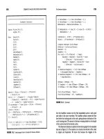
instructions. Figure 1.1a displays the starting portal of a PuTTY SSH.
When you input an IP address under Host Name (or IP address) such as
10.250.20.231, select Protocol SSH, and then click Open; a login screen
will appear. After successful login, you are at the input prompt $ as shown
in Figure 1.1b and the shell is ready to receive proper command or execute
a script.

1.2.2 Basic Linux Commands

</div>
(28)<div class='page_container' data-page=28>

(a) (b)

FIGURE 1.1 Screenshots of a PuTTy confirmation (a) and a valid login to Linux (b).

TABLE 1.1 Common Basic Linux Commands

Category Command Description Example

File administration ls List files ls -al, list all file in detail
cp Copy source file to

target file cp myfile yourfile

rm Remove files or

directories (rmdir or
rm -r)

rm accounts.txt, to remove
the file “accounts.txt” in the
current directory

cd Change current

directory cd., to move to the parent directory of the current
directory

mkdir Create a new directory mkdir mydir, to create a new
directory called mydir
gzip/gunzip Compress/uncompress

the contents of files gzip .swp, to compress the file .swp
Access file contents cat Display the full

contents of a file cat Mary.py, to display the full content of the file
“Mary.py”

Less/more Browse the contents of

the specified file less huge-log-file.log, to browse the content of
huge-log-file.log
Tail/head Display the last or the

first 10 lines of a file
by default

tail -n N filename.txt, to
display N number of lines
from the file named
filename.txt

find Find files find ~ -size -100M, To find

</div>
(29)<div class='page_container' data-page=29>

followed by the name of the command, for example, man ls, which will 
show how to list files in various ways.

1.2.3 File Access Permission

On Linux and other Unix-like operating systems, there is a set of rules for
each file, which defines who can access that file and how they can access it.
These rules are called file permissions or file modes. The command name 
chmod stands for change mode, and it is used to define the way a file can be 
accessed. For example, if one issues a command line to a file named Mary.py
like chmod 765 Mary.py, the permission is indicated by -rwxrw-r-x, which

allows the user to read (r), write (w), and execute (x), the group to read and
write, and any other to read and execute the file. The chmod numerical
format (octal modes) is presented in Table 1.2.

1.2.4 Linux Text Editors

Text editors are needed to write scripts. There are a number of available
text editors such as Emacs, Eclipse, gEdit, Nano, Pico, and Vim. Here we
briefly introduce Vim, a very popular Linux text editor. Vim is the editor
of choice for many developers and power users. It is based on the vi editor
written by Bill Joy in the 1970s for a version of UNIX. It inherits the key
bindings of vi, but also adds a great deal of functionality and extensibility
that are missing from the original vi. You can start Vim editor by typing
vim followed with a file name. After you finish the text file, you can type

TABLE 1.1 (CONTINUED) Common Basic Linux Commands

Category Command Description Example

grep Search for a specific
string in the specified
file

grep “this” demo_file, to
search “this” containing
sentences from the
“demo_file”

Processes top Provide an ongoing

look at processor
activity in real time

top –s, to work in secure
mode

kill Shut down a process kill -9, to send a KILL signal
instead of a TERM signal
System information df Display disk space df –H, to show the number

of occupied blocks in
human-readable format
free Display information

about RAM and swap
space usage

</div>
(30)<div class='page_container' data-page=30>

semicolon (:) plus a lower case letter x to save the file and exit Vim editor.
Table 1.3 lists the most common basic commands used in the Vim editor.

1.2.5 Keyboard Shortcuts

The command line can be quite powerful, but typing in long commands
or file paths is a tedious process. Here are some shortcuts that will have
you running long, tedious, or complex commands with just a few
key-strokes (Table 1.4). If you plan to spend a lot of time at the command line,
these shortcuts will save you a ton of time by mastering them. One should
become a computer ninja with these time-saving shortcuts.

1.2.6 Write Shell Scripts

A shell script is a computer program or series of commands written in
plain text file designed to be run by the Linux/Unix shell,
a command-line interpreter. Shell scripts can automate the execution of repeated tasks
and save lots of time. Shell scripts are considered to be scripting languages

TABLE 1.3 Common Basic Vim Commands

Key Description

h Moves the cursor one character to the left
l Moves the cursor one character to the right
j Moves the cursor down one line

k Moves the cursor up one line

o Moves the cursor to the beginning of the line
$ Moves the cursor to the end of the line

w Move forward one word

b Move backward one word

G Move to the end of the file
gg Move to the beginning of the file

TABLE 1.2 The chmod Numerical Format (Octal Modes)

Number Permission rwx

7 Read, write, and execute 111

6 Read and write 110

5 Read and execute 101

4 Read only 100

3 Write and execute 011

2 Write only 010

1 Execute only 001

0 None 000

</div>
(31)<div class='page_container' data-page=31>

or programming languages. The many advantages of writing shell scripts
include easy program or file selection, quick start, and interactive
debug-ging. Above all, the biggest advantage of writing a shell script is that the
commands and syntax are exactly the same as those directly entered at the
command line. The programmer does not have to switch to a totally
differ-ent syntax, as they would if the script was written in a differdiffer-ent language
or if a compiled language was used. Typical operations performed by shell
scripts include file manipulation, program execution, and printing text.
Generally, three steps are required to write a shell script: (1) Use any
edi-tor like Vim or others to write a shell script. Type vim first in the shell
prompt to give a file name first before entering the vim. Type your first
script as shown in Figure 1.2a, save the file, and exit Vim. (2) Set execute

TABLE 1.4 Common Linux Keyboard Shortcut Commands

Key Description

Tab Autocomplete the command if there is only one option
↑ Scroll and edit the command history

Ctrl + d Log out from the current terminal
Ctrl + a Go to the beginning of the line
Ctrl + e Go to the end of the line
Ctrl + f Go to the next character
Ctrl + b Go to the previous character
Ctrl + n Go to the next line

Ctrl + p Go to the previous line
Ctrl + k Delete the line after cursor
Ctrl + u Delete the line before cursor

Ctrl + y Paste

(a)
#

# My first shell script
#

clear

echo “Next generation DNA sequencing increases the speed and reduces the cost of
DNA sequencing relative to the first generation DNA sequencing.”

(b)

Next generation DNA sequencing increases the speed and reduces the cost of DNA
sequencing relative to the first generation DNA sequencing

</div>
(32)<div class='page_container' data-page=32>

permission for the script as follows: chmod 765 first, which allows the user
to read (r), write (w), and execute (x), the group to read and write, and any
other to read and execute the file. (3) Execute the script by typing: ./first.
The full script will appear as shown in Figure 1.2b.

1.3 STEP-BY-STEP TUTORIAL ON NEXT- GENERATION

SEQUENCE DATA ANALYSIS BY RUNNING

BASIC LINUX COMMANDS

By running Linux commands, this tutorial demonstrates a step-by-step
general procedure for next-generation sequence data analysis by first
retrieving or downloading a raw sequence file from NCBI/NIH Gene
Expression Omnibus (GEO, second,
exercising quality control of sequences; third, mapping sequencing reads
to a reference genome; and fourth, visualizing data in a genome browser.
This tutorial assumes that a user of a desktop or laptop computer has an
Internet connection and an SSH such as PuTTY, which can be logged onto
a Linux-based high-performance computer cluster with needed software
or programs. All the following involved commands in this tutorial are
supposed to be available in your current directory, like /home/username.
It should be mentioned that this tutorial only gives you a feel on
next-gen-eration sequence data analysis by running basic Linux commands and it
won’t cover complete pipelines for next-generation sequence data analysis,
which will be detailed in subsequent chapters.

1.3.1 Step 1: Retrieving a Sequencing File

After finishing the sequencing project of your submitted samples (patient
DNAs or RNAs) in a sequencing core or company service provider, often
you are given a URL or ftp address where you can download your data.
Alternatively, you may get sequencing data from public repositories such
as NCBI/NIH GEO and Short Read Archives (SRA, .
nih.gov/sra). GEO and SRA make biological sequence data available to the
research community to enhance reproducibility and allow for new
discov-eries by comparing data sets. The SRA store raw sequencing data and
align-ment information from high-throughput sequencing platforms, including
Roche 454 GS System®, Illumina Genome Analyzer®, Applied Biosystems

SOLiD System®, Helicos Heliscope®, Complete Genomics®, and Pacific

Biosciences SMRT®. Here we use a demo to retrieve a short-read

</div>
(33)<div class='page_container' data-page=33>

1.3.1.1 Locate the File

Go to the GEO site ( → select Search
GEO Datasets from the dropdown menu of Query and Browse → type
GSE45732 in the Search window → click the hyperlink (Gene expression
analysis of breast cancer cell lines) of the first choice → scroll down to
the bottom to locate the SRA file (SRP/SRP020/SRP020493) prepared for
ftp download → click the hyperlynx(ftp) to pinpoint down the detailed
ftp address of the source file (SRR805877, .
gov/sra/sra-instant/reads/ByStudy/sra/SRP%2FSRP020%2FSRP020493/
SRR805877/).

1.3.1.2 Downloading the Short-Read Sequencing File 
(SRR805877) from NIH GEO Site

Type the following command line in the shell prompt: “wget ftp://ftp-trace.
ncbi.nlm.nih.gov/sra/sra-instant/reads/ByStudy/sra/SRP%2FSRP020%
2FSRP020493 /SRR805877/SRR805877.sra.”

1.3.1.3 Using the SRA Toolkit to Convert .sra Files into .fastq Files

FASTQ format is a text-based format for storing both a biological sequence

(usually nucleotide sequence) and its corresponding quality scores. It has
become the de facto standard for storing the output of high-throughput 
sequencing instruments such as the Illumina’s HiSeq 2500 sequencing system.
Type “fastq-dump SRR805877.sra” in the command line. SRR805877.fastq
will be produced. If you download paired-end sequence data, the parameter
“-I” appends read id after spot id as “accession.spot.readid” on defline and the
parameter “--split-files” dump each read into a separate file. Files will receive a
suffix corresponding to its read number. It will produce two fastq files
(--split-files) containing “.1” and “.2” read suffices (-I) for paired-end data.

1.3.2 Step 2: Quality Control of Sequences

Before doing analysis, it is important to ensure that the data are of high
quality. FASTQC can import data from FASTQ, BAM, and Sequence
Alignment/Map (SAM) format, and it will produce a quick overview to
tell you in which areas there may be problems, summary graphs, and
tables to assess your data.

1.3.2.1 Make a New Directory “Fastqc”

</div>
(34)<div class='page_container' data-page=34>

1.3.2.2 Run “Fastqc”

Type “fastqc -o Fastqc/SRR805877.fastq” in the command line, which will
run Fastqc to assess SRR805877.fastq quality. Type “Is -l Fastqc/,” you will
see the results in detail.

1.3.3 Step 3: Mapping Reads to a Reference Genome

At first, you need to prepare genome index and annotation files. Illumina
has provided a set of freely downloadable packages that contain
bow-tie indexes and annotation files in a general transfer format (GTF) from
UCSC Genome Browser Home (genome.ucsc.edu).

1.3.3.1 Downloading the Human Genome and 
Annotation from Illumina iGenomes

Type “wget ftp://igenome:/Homo_
sapiens/UCSC/hg19/Homo_sapiens_UCSC_hg19.tar.gz” and download
those files.

1.3.3.2 Decompressing .tar.gz Files

Type “tar -zxvf Homo_sapiens_Ensembl_GRCh37.tar.gz” for extracting
the files from archive.tar.gz.

1.3.3.3 Link Human Annotation and Bowtie Index 
to the Current Working Directory

Type “In -s homo.sapiens/UCSC/hg19/Sequence/WholeGenomeFasta/

genome.fa genome.fa”; type “In -s homo.sapiens/UCSC/hg19/Sequence/
Bowtie2Index/genome.1.bt2 genome.1.bt2”; type “In -s homo.sapiens/
UCSC/hg19/Sequence/Bowtie2Index/genome.2.bt2 genome.2.bt2”; type
“In -s homo.sapiens/UCSC/hg19/Sequence/Bowtie2Index/genome.3.bt2
genome.3.bt2”; type “In -s homo.sapiens/UCSC/hg19/Sequence/Bowtie2
Index/genome.4.bt2 genome.4.bt2”; type “In -s homo.sapiens/UCSC/hg19/
Sequence/Bowtie2Index/genome.rev.1.bt2 genome.rev.1.bt2”; type “In -s
homo.sapiens/UCSC/hg19/Sequence/Bowtie2Index/genome.rev.2.bt2
genome.rev.2.bt2”; and type “In -s homo.sapiens/UCSC/hg19/Annotation/
Genes/genes.gtf genes.gtf.”

1.3.3.4 Mapping Reads into Reference Genome

</div>
(35)<div class='page_container' data-page=35>

1.3.4 Step 4: Visualizing Data in a Genome Browser

The primary output of TopHat are the aligned reads BAM file and
junc-tions BED file, which allows read alignments to be visualized in genome
browser. A BAM file (*.bam) is the compressed binary version of a SAM
file that is used to represent aligned sequences. BED stands for Browser
Extensible Data. A BED file format provides a flexible way to define the data 
lines that can be displayed in an annotation track of the UCSC Genome
Browser. You can choose to build a density graph of your reads across
the genome by typing the command line: “genomeCoverageBed -ibam
tophat/accepted_hits.bam -bg -trackline -trackopts ‘name=“SRR805877”
color=250,0,0’>SRR805877.bedGraph” and run. For convenience, you
need to transfer these output files to your desktop computer’s hard drive.

1.3.4.1 Go to Human (Homo sapiens) Genome Browser Gateway

You can load bed or bedGraph into the UCSC Genome Browser to

visu-alize your own data. Open the link in your browser: c.
edu/cgi-bin/hgGateway?hgsid=409110585_zAC8Aks9YLbq7YGhQiQtw
nOhoRfX&clade=mammal&org=Human&db=hg19.

1.3.4.2 Visualize the File

Click on add custom tracks button → click on Choose File button, and
select your file → click on Submit button → click on go to genome browser.
BED files will provide the coordinates of regions in a genome; most
basi-cally chr, start, and end. bedGraph files can give coordinate information
as in BED files and coverage depth of sequencing over a genome.

BIBLIOGRAPHY

1. Haas, J. Linux, the Ultimate Unix, 2004, 
a/linux_2.htm.

2. Gite, VG. Linux Shell Scripting Tutorial v1.05r3-A Beginner’s Handbook, 
1999–2002, />

3. Brockmeier, J.Z. Vim 101: A Beginner’s Guide to Vim, 2009, http://www.

linux.com/learn/tutorials/228600-vim-101-a-beginners-guide-to-vim.

4. Chris Benner et al. HOMER (v4.7), Software for motif discovery and next

generation sequencing analysis, August 25, 2014, />

homer/basicTutorial/.

5. Shotts, WE, Jr. The Linux Command Line: A Complete Introduction, 1st ed.,

No Starch Press, January 14, 2012.

6. Online listing of free Linux books.

</div>
(36)<div class='page_container' data-page=36>

15

C h a p t e r

2 Python for Big

Data Analysis

Dmitry N. Grigoryev

2.1 INTRODUCTION TO PYTHON

Python is a powerful, flexible, open-source programming language that is
easy to use and easy to learn. With the help of Python you will be able to
manipulate large data sets, which is hard to do with common data
oper-ating programs such as Excel. But saying this, you do not have to give
up your friendly Excel and its familiar environment! After your Big Data
manipulation with Python is completed, you can convert results back to
your favorite Excel format. Of course, with the development of technology
at some point, Excel would accommodate huge data files with all known
genetic variants, but the functionality and speed of data processing by
Python would be hard to match. Therefore, the basic knowledge of
pro-gramming in Python is a good investment of your time and effort. Once
you familiarize yourself with Python, you will not be confused with it or
intimidated by numerous applications and tools developed for Big Data
analysis using Python programming language.

2.1 Introduction to Python 15

2.2 Application of Python 16

2.3 Evolution of Python 16

2.4 Step-By-Step Tutorial of Python Scripting in UNIX

and Windows Environments 17

2.4.1 Analysis of FASTQ Files 17

2.4.2 Analysis of VCF Files 21

</div>
(37)<div class='page_container' data-page=37>

2.2 APPLICATION OF PYTHON

There is no secret that the most powerful Big Data analyzing tools are
written in compiled languages like C or java, simply because they run
faster and are more efficient in managing memory resources, which is
cru-cial for Big Data analysis. Python is usually used as an auxiliary language
and serves as a pipeline glue. The TopHat tool is a good example of it [1]. 
TopHat consists of several smaller programs written in C, where Python
is employed to interpret the user-imported parameters and run small C
programs in sequence. In the tutorial section, we will demonstrate how to
glue together a pipeline for an analysis of a FASTQ file.

However, with fast technological advances and constant increases in
computer power and memory capacity, the advantages of C and java have

become less and less obvious. Python-based tools have started taking over
because of their code simplicity. These tools, which are solely based on
Python, have become more and more popular among researchers. Several
representative programs are listed in Table 2.1.

As you can see, these tools and programs cover multiple areas of Big
Data analysis, and number of similar tools keep growing.

2.3 EVOLUTION OF PYTHON

Python’s role in bioinformatics and Big Data analysis continues to grow.
The constant attempts to further advance the first-developed and most
popular set of Python tools for biological data manipulation, Biopython
(Table 2.1), speak volumes. Currently, Biopython has eight actively
devel-oping projects ( several of
which will have potential impact in the field of Big Data analysis.

TABLE 2.1 Python-Based Tools Reported in Biomedical Literature

Tool Description Reference

Biopython Set of freely available tools for biological

computation Cock et al. [2]

Galaxy An open, web-based platform for data intensive

biomedical research Goecks et al. [3]

msatcommander Locates microsatellite (SSR, VNTR, &c) repeats

within FASTA-formatted sequence or
consensus files

Faircloth et al. [4]

RseQC Comprehensively evaluates high-throughput

sequence data especially RNA-seq data Wang et al. [5]
Chimerascan Detects chimeric transcripts in high-throughput

</div>
(38)<div class='page_container' data-page=38>

The perfect example of such tool is a development of a generic feature
format (GFF) parser. GFF files represent numerous descriptive features
and annotations for sequences and are available from many
sequenc-ing and annotation centers. These files are in a TAB delimited format,
which makes them compatible with Excel worksheet and, therefore, more
friendly for biologists. Once developed, the GFF parser will allow analysis
of GFF files by automated processes.

Another example is an expansion of Biopython’s population genetics
(PopGen) module. The current PopGen tool contains a set of applications
and algorithms to handle population genetics data. The new extension of
PopGen will support all classic statistical approaches in analyzing 
popula-tion genetics. It will also provide extensible, easy-to-use, and future-proof
framework, which will lay ground for further enrichment with newly
developed statistical approaches.

As we can see, Python is a living creature, which is gaining popularity
and establishing itself in the field of Big Data analysis. To keep abreast
with the Big Data analysis, researches should familiarize themselves with
the Python programming language, at least at the basic level. The

follow-ing section will help the reader to do exactly this.

2.4 STEP-BY-STEP TUTORIAL OF PYTHON SCRIPTING

IN UNIX AND WINDOWS ENVIRONMENTS

Our tutorial will be based on the real data (FASTQ file) obtained with
Ion Torrent sequencing (www.lifetechnologies.com). In the first part of
the tutorial, we will be using the UNIX environment (some tools for
pro-cessing FASTQ files are not available in Windows). The second part of the
tutorial can be executed in both environments. In this part, we will revisit
the pipeline approach described in the first part, which will be
demon-strated in the Windows environment. The examples of Python utility in
this tutorial will be simple and well explained for a researcher with
bio-medical background.

2.4.1 Analysis of FASTQ Files

</div>
(39)<div class='page_container' data-page=39>

and also ask to have the reference genome and tools listed in Table 2.2
installed. Once we have everything in place, we can begin our tutorial
with the introduction to the pipelining ability of Python. To answer the
potential question of why we need pipelining, let us consider the
fol-lowing list of required commands that have to be executed to analyze a
FASTQ file. We will use a recent publication, which provides a resource
of benchmark SNP data sets [7] and a downloadable file bb17523_PSP4_
BC20.fastq from
exome. To use this file in our tutorial, we will rename it to test.fastq.

In the meantime, you can download the human hg19 genome from
Illumina iGenomes (ftp://igenome:/
Homo_sapiens/UCSC/hg19/Homo_sapiens_UCSC_hg19.tar.gz). The files

are zipped, so you need to unpack them.

In Table 2.2, we outline how this FASTQ file should be processed.
Performing the steps presented in Table 2.2 one after the other is a
labo-rious and time-consuming task. Each of the tools involved will take
some-where from 1 to 3 h of computing time, depending on the power of your
computer. It goes without saying that you have to check on the progress of
your data analysis from time to time, to be able to start the next step. And,
of course, the overnight time of possible computing will be lost, unless
somebody is monitoring the process all night long. The pipelining with
Python will avoid all these trouble. Once you start your pipeline, you can
forget about your data until the analysis is done, and now we will show
you how.

For scripting in Python, we can use any text editor. Microsoft (MS) Word
will fit well to our task, especially given that we can trace the whitespaces of

TABLE 2.2 Common Steps for SNP Analysis of Next-Generation Sequencing Data

Step Tool Goal Reference

1 Trimmomatic To trim nucleotides with bad quality from the

ends of a FASTQ file Bolger et al. [8]

2 PRINSEQ To evaluate our trimmed file and select reads

with good quality Schmieder et al. [9]

3 BWA-MEM To map our good quality sequences to a

reference genome Li et al. [10]

SAMtools To generate a BAM file and sort it Li et al. [11]

5 To generate a MPILEUP file

</div>
(40)<div class='page_container' data-page=40>

our script by making them visible using the formatting tool of MS Word.
Open a new MS Word document and start programming in Python! To
create a pipeline for analysis of the FASTQ file, we will use the Python
col-lection of functions named subprocess and will import from this colcol-lection
function call.

The first line of our code will be

from subprocess import call

Now we will write our first pipeline command. We create a variable, which
you can name at will. We will call it step_1 and assign to it the desired
pipeline command (the pipeline command should be put in quotation
marks and parenthesis):

step_1 = (“java -jar ~/programs/Trimmomatic-0.32/
trimmomatic-0.32.jar SE -phred33 test.fastq test_trmd.
fastq LEADING:25 TRAILING:25 MINLEN:36”)

Note that a single = sign in programming languages is used for an
assign-ment stateassign-ment and not as an equal sign. Also note that whitespaces are very

important in UNIX syntax; therefore, do not leave any spaces in your file
names. Name your files without spaces or replace spaces with underscores,
as in test_trimmed.fastq. And finally, our Trimmomatic tool is located in
the programs folder, yours might have a different location. Consult your 
administrator, where all your tools are located.

Once our first step is assigned, we would like Python to display variable
step_1 to us. Given that we have multiple steps in our pipeline, we would
like to know what particular step our pipeline is running at a given time.
To trace the data flow, we will use print() function, which will display on
the monitor what step we are about to execute, and then we will use call()
function to execute this step:

print(step_1)

call(step_1, shell = True)

</div>
(41)<div class='page_container' data-page=41>

from subprocess import call

step_1 = (“java -jar ~/programs/Trimmomatic-0.32/
trimmomatic-0.32.jar SE -phred33 test.fastq test_
trimmed.fastq LEADING:25 TRAILING:25 MINLEN:36”)
print(step_1)

call(step_1, shell = True)

step_2 = (“perl ~/programs/prinseq-lite-0.20.4/
prinseq-lite.pl -fastq test_trimmed.fastq -min_qual_
mean 20 -out_good test_good”)

print(step_2)

call(step_2, shell = True)

step_3 = (“bwa mem -t 20 homo.sapiens/UCSC/hg19/
Sequence/BWAIndex/genome.fa test_good.fastq > test_
good.sam”)

print(step_3)

call(step_3, shell = True)

step_4 = (“samtools view –bS test_good.sam > test_
good.bam”)

print(step_4)

call(step_4, shell = True)

step_5 = (“samtools sort test_good.bam 
test_good_sorted”)

print(step_5)

call(step_5, shell = True)

step_6 = (“samtools mpileup –f homo.sapiens/UCSC/
hg19/Sequence/WholeGenomeFasta/genome.fa test_good_
sorted.bam > test_good.mpileup”)

print(step_6)

call(step_6, shell = True)

step_7 = (“java -jar ~/programs/VarScan.v2.3.6.jar
mpileup2snp test_good.mpileup --output-vcf 1 > 
test. vcf”)

print(step_7)

call(step_7, shell = True)

Now we are ready to go from MS Word to a Python file. In UNIX, we will
use vi text editor and name our Python file pipeline.py, where extension
.py will tell that this is a Python file.

In UNIX command line type: vi pipeline.py

</div>
(42)<div class='page_container' data-page=42>

button and select from the popup menu Paste. While inside the vi text editor,
turn off the INSERT mode by pressing the Esc key. Then type ZZ, which will
save and close pipeline.py file. The quick tutorial for the vi text editor can be
found at />

Once our pipeline.py file is created, we will run it with the command:

python pipeline.py

This script is universal and should processs any FASTQ file.

2.4.2 Analysis of VCF Files

To be on the same page with those who do not have access to UNIX and
were not able to generate their own VCF file, we will download the premade
VCF file TSVC_variants.vcf from the same source (.
gov/giab/ftp/data/NA12878/ion_exome), and will rename it to test.vcf.

From now on we will operate on this test.vcf file, which can be analyzed
in both UNIX and Windows environments. You can look at this test.vcf
files using the familiar Excel worksheet. Any Excel version should
accom-modate our test.vcf file; however, if you try to open a bigger file, you might
encounter a problem. Excel will tell that it cannot open the whole file. If
you wonder why, the answer is simple. If, for example, you are working
with MS Excel 2013, the limit of rows for a worksheet in this version will
be 1,048,576. It sounds like a lot, but wait, to accommodate all SNPs from
the whole human genome the average size of a VCF file will need to be up
to 1,400,000 rows [13]. Now you realize that you have to manipulate your
file by means other than Excel. This is where Python becomes handy. With
its help you can reduce the file size to manageable row numbers and at
the same time retain meaningful information by excluding rows without
variant calls.

</div>
(43)<div class='page_container' data-page=43>

fantasy desires. We will keep it simple and name it file. Now we will use
function open() to open our file. To make sure that this file will not be
accidently altered in any way, we will use argument of open() function ‘r’,
which allows Python only to read this file. At the same time, we will
cre-ate an output file and call it newfile. Again, we will use function open() to
create our new file with name test_no_description_1.vcf. To tell Python
that it can write to this file, we will use argument of open() function ‘w’:

file = open(“test.vcf”,‘r’)

newfile = open(“test_no_description_1.vcf”,‘w’)

Now we will create all variables that are required for our task. In this
script, we will need only two of them. One we will call line and the other—

n, where line will contain information about components of each row in

test.vcf, and n will contain information about the sequential number of a 
row. Given that line is a string variable (contains string of characters), we
will assign to it any string of characters of your choosing. Here we will
use “abc.” This kind of variable is called character variable and its content 
should be put in quotation marks. The n variable on the other hand will be 
a numeric variable (contains numbers); therefore, we will assign a number 
to it. We will use it for counting rows, and given that we do not count any
rows yet, we assign 0 to n without any quotation marks.

line = “abc”
n = 0

Now we are ready for the body of the script. Before we start, we have to
outline the whole idea of the script function. In our case, the script should
read the test.vcf file line by line and write all but the first 64 lines to a new
file. To read the file line by line, we need to build a repetitive structure—in
programming world this is called loops. There are several loop structures 
in Python, for our purpose we will use the “while” structure. A Python
while loop behaves quite similarly to common English. Presumably, you
would count the pages of your grant application. If a page is filled with
the text from top to bottom, you would count this page and go to the next
page. As long as your new page is filled up with the text, you would repeat
your action of turning pages until you reach the empty page. Python has a

similar syntax: while line != “”:

</div>
(44)<div class='page_container' data-page=44>

block of code (body of the loop). Note that each statement in Python (in
our case looping statement) should be completed with the colon sign (:).
Actually, this is the only delimiter that Python has. Python does not use
delimiters such as curly braces to mark where the function code starts
and stops as in other programming languages. What Python uses instead
is indentations. Blocks of code in Python are defined by their
indenta-tion. By block of code, in our case we mean the content of the body of our 
“while” loop. Indenting the starts of a block and unindenting ends it. This
means that whitespaces in Python are significant and must be consistent.
In our example, the code of loop body will be indented six spaces. It does
not need to be exactly six spaces, it has to be at least one, but once you have
selected your indentation size, it needs to be consistent. Now we are going
to populate out while loop. As we have decided above, we have to read the
content of the first row from test.vcf. For this we will use function
read-line(). This function should be attached to a file to be read via a point sign.
Once evoked, this function reads the first line of provided file into variable
line and automatically jumps to the next line in the file.

line = file.readline()
n = n + 1

To keep track of numbers for variable line, we started up our counter n.
Remember, we set n to 0. Now our n is assigned number 1, which 
corre-sponds to our row number. With each looping, n will be increasing by 1 
until the loop reaches the empty line, which is located right after the last
populated line of test.vcf.

Now we have to use another Python structure: if-else statement.

if n <= 64:
continue
else:

newfile.write(line)

</div>
(45)<div class='page_container' data-page=45>

the colon (:). The block of if statement (in our case continue) is indented,
which means that it will be executed only when the condition in the if
statement is true. Once we went over the line number 64, we want the
rest of the test.vcf file to be written to our new file. Here we used the
write() function. As with readline() function, we attached write()
func-tion to a file to be written to via a point sign. Inside of the parenthesis
of a function, we put the argument line to let the function know what
to write to the newfile. Note that the logical else statement is also
com-pleted with the colon (:). The block of else statement (newfile.write(line)
in our case) is indented, which means that it will be executed only when
the original condition, if n <= 64, is false. In an if-else statement, only 
one of two indented blocks can be executed. Once we run our loop and
generated a file, which does not have 64 descriptive rows in it, we can
close both original and newly generated files. To do this, we will use
function close(). Once again, we will attach close() function to a file to
be closed via a point sign.

newfile.close()
file.close()

</div>
(46)<div class='page_container' data-page=46>

Make sure that your step_1a.py file and test.vcf file are located in the
same directory. Once we have familiarized ourselves with Python
script-ing, we will move to a more complex task. As we said above, there are

two ways to code for removing descriptive rows from a VCF file. One can
ask: why do we need another approach to perform this file modification?
The answer is: not all VCF files are created in the same way. Although,
by convention, all descriptive rows in VCF files begin with double pound
sign (##), the number of descriptive rows varies from one sequence
align-ing program to another. For instance, VСF files generated by Genome
Analysis Toolkit for FASTQ files from Illumina platform have 53
tive rows [13] and our pipeline described above will generate 23
descrip-tive rows. Of course, we can change our logical statement if n <= 64: to 
if n <= 53: or if n <= 23:, but why do not make our code universal? We 
already know that each descriptive row in VCF files begin with ## sign;
therefore, we can identify and remove them. Given that we are planning
to manipulate on the row content, we have to modify our loop. Our
previ-ous script was taking the empty row at the end of the test.vcf file and was
writing it to the test_no_description_1.vcf file without looking into the
row content. Now, when we operate on the content of a row, Python will
complain about the empty content and will report an error. To avoid this,
we have to make sure that our script does not operate with the empty row.
To do this, we will check whether the row is empty beforehand, and if it is,
we will use break statement to abort our script. Once again, our code will

</div>
(47)<div class='page_container' data-page=47>

be close to English. Assume you are proofreading your completed grant
application. If you reach the end of it and see the empty page, you are done
and deserve a break.

if line == “”:
break

As you might have noticed, we used just part of the if-else statement, which
is perfectly legal in Python. Once our program reaches the end of the file,

there is nothing else to do but stop the script with break statement;
there-fore, there is no need for any else. And another new sign double equal (==)
stands for a regular equal. Note that even the shortened if-else statement 
should be completed with the colon (:). The block of the if statement (in our
case break) also should be indented, which means that it will be executed
only when the condition in the if statement is true. Now, when we created
internal break, we do not need the redundant check point at the beginning
of our loop. Therefore, we will replace while line != “”: with while 1:. Here
we have introduced the “infinite” loop. The statement while 1 will run our
loop forever unless we stop it with a break statement. Next, we will modify
our existing if-else statement. Given that now we are searching for a ##
pattern inside the row, rather than simply counting rows, we will replace

if n <= 64:
with

if line[1] == “#”:

With line[1], we introduce the process of counting row content in Python.
The line variable here represents the whole row of test.vcf file. To
visual-ize content of a line variable, you can simply display it on your computer
screen with print() function using line as an argument.

file = open(“test.vcf”,‘r’)
line = file.readline()
print(line)

</div>
(48)<div class='page_container' data-page=48>

number into square brackets, for example, command print(line[1]) will
display the second # sign. This is our mark for the descriptive rows;
there-fore, whenever our script sees line[1] as #, it will skip this row and go to the

next one. Our complete modified script will look like this now:

print(“START”)

file = open(“test.vcf”,‘r’)

newfile = open(“test_no_description_2.vcf”,‘w’)
line = “abc”

while 1:

line = file.readline()
if line == “”:

break

if line[1] == “#”:
continue
else:

newfile.write(line)
newfile.close()

file.close()
print(“END”)

Now we can copy and paste our script either into vi text editor (UNIX) or
into Python GUI Shell (Windows), save it as step_1b.py and run. Once we
are done with cutting out the descriptive rows, we can further simplify and
reduce the size of our VCF file. We will use our previous script as template,

and for the beginning, we will change our input and output files. Given that
our goal is to make original VCF file the Excel compatible, we will use text
format for our output file and will add to the file name an extension .txt.

file = open(“test_no_description_2.vcf”,‘r’)
newfile = open(“alleles.txt”,‘w’)

Our alleles.txt will have not only a different extension but also a different
content. The most efficient way for researchers to operate on the allelic
distribution data is to know the allelic variant location and variant itself.
Therefore, our new file will have only three columns: chromosome
num-ber, position of a variant on this chromosome, and allelic distribution of
the variant. As a reminder of which part of our script was doing what,
we will use comments inside of our script. Typically, the pound sign (#)
is used in front of comment. In the programming world, it is called

</div>
(49)<div class='page_container' data-page=49>

# Creating columns titles for newfile

line = file.readline()

newfile.write(“Chromosome” + “\t” + “Position” + “\t” + 
“Alleles” + “\n”)

Given that columns in text formatted files are separated by the TAB sign
(\t), we separated our titles with “\t,” and, as we learned by now, all textual
entries in Python should have quotation marks. We also have to end the
title row with the NEWLINE sign (\n), which tells Python that this row
is completed and any further input should go to the next row. Once we
are done with formatting our output file, we will restructure our existing
if-else statement by adding new variable. This variable (we will call it rec)

will keep record of each column content after we split a row by columns.
To manipulate the row content on column-by-column bases, we will need
a package of functions specifically designed to do exactly this. The package
is called string. In our first pipeline exercise, we already had an experience
with importing call function; here in the same fashion, we will import
string using an identical Python statement: import string.

Now we are set to operate on the row content. Before we begin, we have
to check how many columns the file we are going to operate on has. By
convention, a VCF file has nine mandatory columns, and then starting
with the tenth column, it will have one sample per column. For simplicity,
in our tutorial, we have a VCF file with just one sample. We also have to
know what kind of column separator is used in our data. By convention, a
VCF file uses tab (\t) as a column separator. Armed with this knowledge,
we can start scripting. First, we read the whole row from our file, assign it
to the variable line, and will make sure that this line is not empty. Then, we
will split the line in pieces according to columns using the string splitting
function str.split():

line = file.readline()
if line == “”:

break

rec = str.split(line,“\t”)

</div>
(50)<div class='page_container' data-page=50>

counting starts with 0. Therefore, the tenth column in our row for Python
will be column number nine. To display the content of the column 10,
where our sample sits, we will use print() function: print(rec[9]).

In our exercise, you will see on your computer screen the following row
of data:

1/1:87:92:91:0:0:91:91:43:48:0:0:43:48:0:0

Before going further, we have to familiarize ourselves with the format of
VCF file. For the detailed explanation of its format, the reader can use
Genome 1000 website (
For our purpose, we will consider only the genotype part of the VCF file,
which is exactly what we are seeing on our screens right now.

Genotype of a sample is encoded as allele values separated by slash
(/). The allele values are 0 for a reference allele (which is provided in the
REF column—column four or rec[3]) and 1 for the altered allele (which
is provided in the ALT column—column five or rec[4]). For homozygote
calls, examples could be either 0/0 or 1/1, and for heterozygotes either
0/1 or 1/0. If a call cannot be made for a sample at a given locus, each
missing allele will be specified with a point sign (./.). With this
knowl-edge in hands, the reader can deduce that in order to identify genotype
of a sample we are going to operate on the first and the third elements of
rec[9] (row of data above), which are representing codes for alleles
iden-tified by sequencing (in our example 1 and 1 or ALT and ALT alleles,
respectively). But once again for Python these are not positions 1 and 3,
but rather 0 and 2; therefore, we tell Python that we would like to work on
rec[9][0] and rec[9][2]. Now we are set with the values to work with and
can resume scripting. First, we will get rid of all meaningless allele calls,
which are coded with points instead of numbers (./.). Using the similar
construction, which we used above for skipping descriptive rows, we will
get this statement:

if rec[9][0] == “.” or rec[9][2] == “.”:
continue

In plain English it says: if the first allele or the second allele is not detected
by a sequencer, we are not interested in this row of data and will continue
with the next row of data. Script will stop performing downstream
com-mands; therefore, this row will not be written to our output alleles.txt file.

</div>
(51)<div class='page_container' data-page=51>

The script will return to the beginning of while loop and will start analysis
of the next row in test_no_description_2.vcf file. Now we have to
con-sider a situation when both alleles were identified by a sequencer and were
assigned corresponding code, either 0 or 1. In this case, the script should
write a new row to our output file. Therefore, we have to start to build
this row beginning with the variant location in the genome. In our input
file, this information is kept in the first two columns “Chromosome” and
“Position,” which are for Python rec[0] and rec[1].

newfile.write(rec[0] + “\t” + rec[1] + “\t”)

Here we follow the same rule as for a title row and separating future
columns by TAB (\t) character. Now we have to populate the third column
of our output file with allelic information. Analyzing structure of our VCF
file, we already figured out that reference allele is corresponding to rec[3]
and altered allele is corresponding to rec[4]. Therefore, our script for
writ-ing first allele will be

# Working with the first allele
if rec[9][0] == “0”:

newfile.write(rec[3])

else:

newfile.write(rec[4])

We comment to ourselves that we are working with the first allele (rec[9] [0]).
These lines of script tell that if an allele is coded by 0, it will be presented in
the “Alleles” column as the reference allele (rec[3]), otherwise (else) it will be
presented as the altered allele (rec[4]). And how do we know that we have
only two choices? Because we have already got rid of non-called alleles (./.)
and the rec[9][0] can only be 0 or 1. The second allele (rec[9][2]) will be
processed in the same fashion (the only difference will be an addition of the
NEWLINE character /n), and our complete script will be as follows:

print(“START”)
import string

file = open(“test_no_description_2.vcf”,‘r’)
newfile = open(“alleles.txt”,‘w’)

line = “abc”

</div>
(52)<div class='page_container' data-page=52>

newfile.write(“Chromosome” + “\t” + “Position” + “\t” +
“Alleles” + “\n”)

while 1:

line = file.readline()
if line == “”:

break

rec = str.split(line,“\t”)

if rec[9][0] == “.” or rec[9][2] == “.”:
continue

newfile.write(rec[0] + “\t” + rec[1] + “\t”)
# Working with the first allele

if rec[9][0] == “0”:

newfile.write(rec[3])
else:

newfile.write(rec[4])
# Working with the second allele
if rec[9][2] == “0”:

newfile.write(rec[3] + “\n”)
else:

newfile.write(rec[4] + “\n”)
newfile.close()

file.close()
print(“END”)

Now we can copy and paste our script either into vi text editor (UNIX) or
into Python GUI Shell (Windows), save it as step_2.py and run. When our
VCF file is shortened by descriptive rows and rows that had no allelic calls,

we will most likely be able to fit it into the Excel worksheet and manipulate
with it in our familiar environment. Once you write your Python scripts
for handling VCF files, you can keep reusing them by just substituting
input and output file names. To make this process even less laborious,
we can join our two-step approach into one script. There are two ways to
handle it. The first one will be to pipeline our scripts as we described in the
beginning of our tutorial.

Let’s create new script both_steps_1.py. We will pipeline our scripts
step1b.py and step2.py using the approach described in our first exercise.

from subprocess import call

command_1 = (“python step_1b.py”)
print(command_1)

</div>
(53)<div class='page_container' data-page=53>

command_2 = (“python step_2.py”)
print(command_2)

call(command_2, shell = True)

This script can be run in both UNIX and Windows environments. The
second way to join step_1b.py and step_2.py scripts is simply to put them
into one common Python script and name it both_steps_2.py. In this way,
we will save some computing time and disk space, because there will be no
need for generating intermediate file test_no_description_2.vcf. However,
the joined script will be more complex in terms of indentation rule. We
have to make sure that flow of our scripts follows the intended route. To
do this, we will put allele selection block of step_2.py script under the else
statement of step_1b.py script:

print(“START”)
import string

file = open(“test.vcf”,‘r’)

newfile = open(“alleles_joined_script.txt”,‘w’)
line = “abc”

#Creating columns titles for newfile
line = file.readline()

newfile.write(“Chromosome” + “\t” + “Position” + “\t” +
“Alleles” + “\n”)

while 1:

line = file.readline()
if line == “”:

break

if line[1] == “#”:
continue
else:

rec = str.split(line,“\t”)

if rec[9][0] == “.” or rec[9][2] == “.”:
continue

newfile.write(rec[0] + “\t” + rec[1] + “\t”)
#working with the first allele

if rec[9][0] == “0”:

newfile.write(rec[3])
else:

newfile.write(rec[4])
#working with the second allele
if rec[9][2] == “0”:

</div>
(54)<div class='page_container' data-page=54>

else:

newfile.write(rec[4] + “\n”)
newfile.close()

file.close()
print(“END”)

This script can be run in both UNIX and Windows environments.
I hope you have enjoyed our tutorial and got a flavor of Python
pro-gramming. You can continue educating yourselves with general (not
Big Data related) tutorials of the usage of Python, which are available
online. A good place to start for real examples is to read about Biopython
(Table 2.1). You will find tutorials there, which use a number of real-life
examples. You can come up with small projects for yourself like writing
a script that analyzes GC content of a FASTA file or a script that parses a
BLAST output file and filter on various criteria.

REFERENCES

1. Trapnell C, Roberts A, Goff L, Pertea G, Kim D, Kelley DR, Pimentel H,
Salzberg SL, Rinn JL, Pachter L: Differential gene and transcript expression
analysis of RNA-seq experiments with TopHat and Cufflinks. Nat Protoc 
2012, 7(3):562–578.

2. Cock PJ, Antao T, Chang JT, Chapman BA, Cox CJ, Dalke A, Friedberg I,
Hamelryck T, Kauff F, Wilczynski B et al.: Biopython: Freely available
Python tools for computational molecular biology and bioinformatics.

Bioinformatics 2009, 25(11):1422–1423.

3. Goecks J, Nekrutenko A, Taylor J: Galaxy: A comprehensive approach for
supporting accessible, reproducible, and transparent computational research
in the life sciences. Genome Biol 2010, 11(8):R86.

4. Faircloth BC: Msatcommander: Detection of microsatellite repeat arrays
and automated, locus-specific primer design. Mol Ecol Resour 2008, 8(1): 
92–94.

5. Wang L, Wang S, Li W: RSeQC: Quality control of RNA-seq experiments.

Bioinformatics 2012, 28(16):2184–2185.

6. Maher CA, Kumar-Sinha C, Cao X, Kalyana-Sundaram S, Han B, Jing X,
Sam L, Barrette T, Palanisamy N, Chinnaiyan AM: Transcriptome
sequenc-ing to detect gene fusions in cancer. Nature 2009, 458(7234):97–101.
7. Zook JM, Chapman B, Wang J, Mittelman D, Hofmann O, Hide W, Salit M:

Integrating human sequence data sets provides a resource of benchmark
SNP and indel genotype calls. Nat Biotechnol 2014, 32(3):246–251.

8. Bolger AM, Lohse M, Usadel B: Trimmomatic: A flexible trimmer for
Illumina sequence data. Bioinformatics 2014, 30(15):2114–2120.

</div>
(55)<div class='page_container' data-page=55>

10. Li H, Durbin R: Fast and accurate short read alignment with
Burrows-Wheeler transform. Bioinformatics 2009, 25(14):1754–1760.

11. Li H, Handsaker B, Wysoker A, Fennell T, Ruan J, Homer N, Marth G,
Abecasis G, Durbin R: The sequence alignment/map format and SAMtools.

Bioinformatics 2009, 25(16):2078–2079.

12. Koboldt DC, Zhang Q, Larson DE, Shen D, McLellan MD, Lin L, Miller CA,
Mardis ER, Ding L, Wilson RK: VarScan 2: Somatic mutation and copy
number alteration discovery in cancer by exome sequencing. Genome Res 
2012, 22(3):568–576.

13. Shortt K, Chaudhary S, Grigoryev D, Heruth DP, Venkitachalam L,
Zhang LQ, Ye SQ: Identification of novel single nucleotide polymorphisms
associated with acute respiratory distress syndrome by exome-seq. PLoS

</div>
(56)<div class='page_container' data-page=56>

35

C h a p t e r

3 R for Big Data Analysis

Stephen D. Simon

3.1 Introduction 36

3.2 R Applications 37

3.2.1 Flexible Storage Choices 37

3.2.2 Objects and Methods 38

3.2.3 Extensibility 39

3.2.4 Graphics 39

3.2.5 Integrated Development Environment 40

3.2.6 Size and Speed Issues 40

3.2.7 Resources for Learning More About R 41

3.3 Data Analysis Outline 42

3.3.1 Import Your Data 42

3.3.2 Manipulate Your Data 42

3.3.3 Screen Your Data 43

3.3.4 Plot Your Data 44

3.3.5 Analyze Your Data 44

3.4 Step-By-Step Tutorial 44

3.4.1 Step 1: Install R, RStudio, and Any R Packages

That You Need 44
3.4.2 Step 2: Import the Son et al. Data 45
3.4.3 Step 3: Select Adrenal Gland Tissue

and Apply a Log Transformation 46
3.4.4 Step 4: Screen Your Data for Missing Values

</div>
(57)<div class='page_container' data-page=57>

3.1 INTRODUCTION

R is both a programming language and an environment for data analysis
that has powerful tools for statistical computing and robust set of
func-tions that can produce a broad range of publication quality graphs and
figures. R is open source and easily extensible with a massive number of
user-contributed packages available for download at the Comprehensive R
Archive Network (CRAN).

R has its roots in a package developed by Richard Becker and John
Chambers at Bell Labs in the 1970s through the 1990s known as S. The
S language had several features that were revolutionary for the time: the
storage of data in self-defining objects and the use of methods for those
objects (Chambers 1999). A commercial version of S, S-plus, was
intro-duced by Statistical Sciences Corporation in the 1990s and became very

popular. Around the same time, Ross Ihaka and Robert Gentleman
devel-oped R, an open source version of S based on the GNU license. Because
R was written mostly in C with a few FORTRAN libraries, it was easily
ported to various Unix systems, the Macintosh, and eventually Microsoft
Windows.

R grew rapidly in popularity and was even highlighted in a major New York

Times article about data analytics (Vance 2009). While there is considerable

debate about the relative popularity of R versus other statistical packages and
programming languages, there is sufficient empirical data to show that R is
currently one of the leaders in the field. For example, R is listed as the fifth
most common programming language in job postings behind Java,
statisti-cal analysis system (SAS), Python, and C/C++/C# (Muenchen 2015). At the
Kaggle website, it is listed as the favorite tool by more competitors than any
other and is cited more than twice as often as the next closest favorite tool,
MATLAB® (Kaggle 2015).

R is currently maintained by the R Foundation for Statistical
Com-puting (www.r-project.org/foundation). It has a robust support network
with hundreds of R bloggers and an annual international conference
(UseR).

3.4.5 Step 5: Plot Your Data 48

3.4.6 Step 6: Analyze Your Data 50

3.5 Conclusion 53

</div>
(58)<div class='page_container' data-page=58>

3.2 R APPLICATIONS

R has many features that make it ideal for modern data analysis. It has
flexible storage choices, object-oriented features, easy extensibility, a
pow-erful integrated development environment, strong graphics, and
high-performance computing enhancements.

3.2.1 Flexible Storage Choices

R has all the commonly used data types (e.g., numeric, character, date,
and logical). Data are assigned using “<-” though more recent versions of
R allow you also to assign using “=”. So x<-12 assigns the numeric value
of 12 to x, and y=TRUE assigns the logical value of TRUE to y.

More than one value of the same type can be combined into a vector using
the c (short for combine) function. So c(1,2,3) would be a numeric vector 
and c(“a”,“b”,“c”) would be a character vector. Sequential vectors can
be produced using the operator or the seq function. 1:50 would produce all
the numbers between 1 and 50 and seq(2,10,by=2) would produce
all the even numbers up to 10.

Vectors of the same length and same type can also be combined in a
matrix. Vectors of the same length (but possibly of different types) can
be combined into a data frame, which is the most common format used
for data analysis in R. A data frame is essentially the same as a table in
database.

But the power of R comes largely from lists. A list liberates the data
set from a restrictive rectangular grid. A list is an ordered set of elements
that can include scalars, vectors of different types and lengths, whole data

frames or matrices, or even other lists. Consider, for example, a
microar-ray experiment. This experiment would contain genotypic information:
expression levels for thousands of genes. It would also contain phenotypic
information, such as demographic information of the patients themselves
or information about the treatments that these patients are receiving.
A third set of information might include parameters under which the
microarray experiment was run. A list that contains a separate data frame
for genotypic and phenotypic information and various scalars to
docu-ment the experidocu-mental conditions provides a simpler and more
manage-able way to store these data than any flat rectangular grid.

</div>
(59)<div class='page_container' data-page=59>

upper left entry (first row, first column) in the matrix or data frame y. 
If you want everything except some entries that you would exclude, place a
negative sign in front. So z[-1,] would produce everything in the matrix z 
except for the very first row.

Subsets for a list are selected the same way except you use a double
bracket. So u[[3]] would be the third element in the list u. If a list has 
names associated with each element, then the $ operator would select the
element with that name. So u$min produces the element of the list u that 
has the name min.

3.2.2 Objects and Methods

Statistical analysis in R is conducted using function calls. The lm function,
for example, produces a linear regression analysis. An important feature of R,
however, is that the function call does not produce output in the sense that a 
program like SAS or Statistical Package for the Social Sciences (SPSS) would.
The function call creates an object of type “lm.” This object is a list with a
pre-specified structure that includes a vector of regression coefficients, a vector of

residuals, the QR decomposition of the matrix of independent variables, the
original function call, and other information relevant to the regression analysis.

Just about every object in R has multiple methods associated with it.
Most objects that store information from a statistical analysis will have
print, plot, and summary methods associated with them. The plot
func-tion for lm objects, for example, will display a graph of the fitted values
versus the residuals, a normal probability plot of the residuals, a
scale-location plot to assess heteroscedasticity, and a plot of leverage versus
residuals. The summary function will produce quartiles of the
residu-als, t-tests for individual coefficients, values for multiple R-squared and 
adjusted R-squared, and an overall F statistic. Objects in R will often
uti-lize inheritance. The “nlm” object, which stores information from a
non-linear regression model, and the “glm” object, which stores information
from a generalized linear model, both inherit from the “lm” object. In
other words, they store much of the same information as an “lm” object
and rely on many of the same methods, but include more information and
have additional methods specific to those more specialized analyses.

</div>
(60)<div class='page_container' data-page=60>

3.2.3 Extensibility

R is easily extensible and has thousands of user-contributed packages,
available at the CRAN ( The R language appears
to be the mode by which most new methodological research in Statistics is
disseminated. Of particular interest to genetics researchers is Bioconductor
( a set of packages devoted to analysis of
genetic data.

There are literally thousands of R packages and you may feel that you
are looking for a needle in a haystack. You should start by reading the

vari-ous task views at CRAN. These task views provide brief explanations of all
the R packages in a particular area like medical imaging.

While anyone can develop a user-contributed package, there are some
requirements for documentation standards and software testing. The
quality of these packages can still be uneven, but you should be able to
trust packages that are documented in peer-reviewed publications. You
should also consider the reputation of the programming team that
pro-duced the R package. Finally, the crantastic website (
has user-submitted reviews for many R packages.

For those who want or need to use other languages and packages as part
of their data analysis, R provides the packages that allow interfaces with
programming languages like C++ (Rcpp) and Python (rPython); Bayesian
Markov Chain Monte Carlo packages like WinBUGS (R2WinBUGS), jags
(rjags, runjags), and Stan (RStan); and data mining packages like Weka
(rWeka).

3.2.4 Graphics

R produces graphics that have intelligent default options. The axes, for
example, are extended 4% on either end before plotting so that points
at the extreme are not partially clipped. The axis labels, by default, use

pretty values that are nice round numbers intelligently scaled to the range

of the data. The default colors in R are reasonable, and you can select a
wide range of color gradients for heat maps and geospatial plots using
the RColorBrewer package. The par function in R allows you to adjust
the graphical parameters down to the level of the length of your axis tick

marks.

</div>
(61)<div class='page_container' data-page=61>

to customize graphs at a high level of abstraction by changing individual
components (Wickham 2010).

The CRAN graphics task view ( />Graphics.html) shows many other R graphics packages, including a link
to the lattice graphics system, which is an R implementation of the trellis
system (Becker et al. 1996).

3.2.5 Integrated Development Environment

You can program in R with a basic text editor (I have used notepad with
R for more years than I care to admit), but there is a very nice integrated
development environment, RStudio, that you should give serious
consid-eration to. It offers code completion, syntax highlighting, and an object
browser. It integrates nicely with version control software and the R
Markdown language.

R Markdown is worth a special mention. An active area of interest
in the Statistics community is the concept of reproducible research.
Reproducible research makes not just the data associated with a research
publication available, but also the code so that other people who want to
do work in this field can easily replicate all of the statistical analyses and
reproduce all of the tables and graphs included in the article (Peng 2009).
The R Markdown language combined with the R package knitr allows you
to produce self-documenting computer output, which greatly enhances
the reproducibility of your publication.

3.2.6 Size and Speed Issues

R can handle many Big Data problems without a fuss, but it has two
well-known limitations. The first limitation is that loops in R are often very
inefficient. The inefficiency is often not noticeable for small data sets,
but loops are commonly a serious bottleneck for Big Data. You can often
improve the speed of your R code by replacing the loop with a function
that works equivalently (Ligges and Fox 2008). There are basic functions
in R for summation (rowSums, colSums) and vector/matrix operators
like crossprod and outer that will run a lot faster and improve the
readability of your code. R also has a series of apply functions that can 
avoid an explicit loop. The sapply function, for example, takes a function
that you specify and applies it to each element in a list.

</div>
(62)<div class='page_container' data-page=62>

iterations in the loop can be run on different processors. The R code
amenable to parallelization in R is limited, but this is an active area of
work in the R community.

A second limitation of R is that it needs to store all available data in
computer memory. These days computer memory is not trivially small, but
it still has limits compared to what you can store on your local hard drive
or your network. If your data are too big to fit in memory, you have to use
special tools. Sometimes you can sidestep the problems with data too big
to fit in memory by handling some of the data management through SQL.
Other times you can reduce the size of your data set through sampling.
You can also use specialized libraries that replace R functions with
equiv-alent functions that can work with data larger than computer memory.
The biglm package, for example, allows you to fit a linear regression model
or a generalized linear regression model to data sets too big to fit in R.

The tools available for improving speed and storage capacity are too
numer-ous to document here. A brief summary of the dozens of R packages that can

help you is listed in the CRAN Task View on High Performance Computing
( />

3.2.7 Resources for Learning More About R

Since R is freely available, many of the resources for learning R are also
free. You should start with the CRAN. CRAN has the official R manuals.
It also has a very helpful FAQ for the overall package and a specialized
FAQ for Windows, Macintosh, and Unix implementations of R. CRAN
also is the repository for most R packages (excluding the packages
ated with Bioconductor), and you can browse the documentation
associ-ated with each package, which is stored in a standardized format in a PDF
file. Some packages have vignettes that show some worked examples.

R has a built-in help system, and selecting help from the menu will
pro-vide an overview of all the resources within R. If you want help with a
par-ticular function, type a question mark followed by the function name or
use the help function. So ?plot or help(“plot”) provides information
about the plot function. If you are not sure what the name of the function
is, you can run a general search using two question marks followed by the
search term, or equivalently, you can use the help.search function.
So ??logistic or help.search(“logistic”) will help you find the
function that performs logistic regression.

</div>
(63)<div class='page_container' data-page=63>

includes one or more data sets that can illustrate how the package is used.
Additional data sets and code in R to analyze these data sets are available at
the Institute for Digital Research and Education at the University of California
at Los Angles ( This site is ideal for those
already familiar with another statistics package like SAS or SPSS because you
can compare the R code with the code from these other packages.

There are hundreds of R bloggers and many of them will repost their blog
entries at the R-bloggers site ( The R help
mail-ing list is available at CRAN ( It is a
very active list with dozens of messages per day. You may find the nabble
interface to be more convenient ( Many
communities have local R user groups. Revolution Analytics offers a fairly
current and comprehensive list of these (http://blog. revolutionanalytics.
com/local-r-groups.html).

3.3 DATA ANALYSIS OUTLINE

Every data analysis is different, but there are some common features for
most analyses. First, you need to import your data. Often, you will need to
manipulate your data in some way prior to data analysis. Then, you need
to screen your data with some simple summary statistics and plots. For the
actual data analysis, it is tempting to start with the largest and most
com-plex model, but you should fit simpler models first, even overly simplistic
models, so that you aren’t immediately overwhelmed.

3.3.1 Import Your Data

R can easily handle a variety of delimited files with the read.table
function and you can also use read.csv, which specializes in reading
the commonly used comma separated value format, and read.delim,
which specializes in reading tab delimited files. The foreign package allows
you to import from a variety of other statistical packages (EpiInfo, SPSS,
SAS, and Systat). The dbi package will connect you with most common
SQL databases and there are specialized packages for Oracle (ROracle)
and SQL Server (RSQLServer). You can sometimes find specialized
pack-ages to handle specific formats like MAGE-ML (RMAGEML). There are

also libraries to import from various social media like Twitter (TwitteR).

3.3.2 Manipulate Your Data

</div>
(64)<div class='page_container' data-page=64>

a many-to-one merge and using either an inner join or an outer join.
Longitudinal data often require you to convert from a format with one
record per subject and data at multiple time points strung out across
hori-zontally to a format with multiple records per subject and one line per
time point within each subject. The reshape2 package makes these
conver-sions easy.

If you need to aggregate your data, you can choose among several
dif-ferent functions (apply, sapply, or tapply) depending on whether
your data are stored in a matrix, a list, or a data frame. These functions
are very powerful, but also rather tricky to work with. For more advanced
aggregation tasks, look at the functions available in the plyr package.

Another common data manipulation is subset selection. There are
several approaches, but often a simple logical expression inserted as an
index within a matrix or data frame will work nicely. The grep function,
which finds matches to strings or regular expressions, is another common
approach for subset selection.

Many data sets have special numeric codes for categorical data. You
will often find that the formal analyses will be easier to follow if you
des-ignate categorical variables using the factor function. This function
also allows you to specify a label for each category value and will simplify
certain regression models by treating factors as categorical rather than
continuous.

3.3.3 Screen Your Data

R has a variety of tools for screening your data. The head function shows
the first few lines of your matrix or data frame, and the tail function
shows the last few lines. The dim function will tell you how many rows or
columns your matrix/data frame has.

If your data are stored in a data frame, the summary function is very
useful. It provides a list of the six most common values for string variables
and factors. For variables that are numeric, summary produces the
mini-mum, 25th percentile, median, mean, 75th percentile, and the maximum
plus a count of the number of missing values if there are any. You need
to watch missing values very carefully throughout the rest of your data
analysis.

</div>
(65)<div class='page_container' data-page=65>

possible values and even if the person who entered the data intended for
them to all mean the same thing, R will treat them as separate values.

3.3.4 Plot Your Data

R has a wide range of plotting methods. For an initial screen, you can
examine simple bivariate relationships using the plot function. Often,
a smooth curve using the lowess function can help you discern patterns
in the plot. The boxplot function helps you to examine the
relation-ship between a categorical variable and a continuous variable. For very
large data sets, some data reduction technique like principal components
or some data summary technique like cluster analysis may prove useful.

3.3.5 Analyze Your Data

The data analysis models are virtually unlimited, and it is impossible to
summarize them here. As a general rule, you should consider the very
simplest models first and then add layers of complexity slowly until you
build up to your final model(s). Do this even if the simplest models are
such oversimplifications that they strain the credulity of the analyses. You
have to spend some time getting comfortable with the data and familiar
with the general patterns that exist. The simplest models help you gain this
comfort and familiarity.

3.4 STEP-BY-STEP TUTORIAL

A gene expression data set freely available on the web gives you the
oppor-tunity to try out some of the features of R. This data set, described in Son
et al. (2005), includes gene expression levels for over 40,000 genes across
158 samples with 19 different organs selected from 30 different patients (not
every patient contributed samples for all 19 organs). For these data, an
anal-ysis of gender differences in the gene expression levels in the adrenal gland
is illustrated. The data are already normalized, reducing some of your work.
The analysis suggested here is somewhat simplistic and you should consider
more sophistication, both in terms of the hypothesis being addressed and in
the data analysis methods. If you are unclear on how any of the functions
used in this example work, review the help file on those functions.

</div>
(66)<div class='page_container' data-page=66>

If you wish to use the integrated development environment RStudio,
download it at You will only need one R
pack-age in this example, mutoss. You can download it by running R and
typ-ing install.packages(“mutoss”) on the command line. You can
also install mutoss from the menu system in R (select Packages|Install
package(s)…).

3.4.2 Step 2: Import the Son et al. Data

The data set that you need to import is found in a tab delimited text file. 
The URL is genome.cshlp.org/content/suppl/2005/02/11/15.3.443.DC1/
Son_etal_158Normal_42k_RatioData.txt. You can read this directly
from R without having to download the file, or you have the option of
downloading the file to your local computer. Here is the code for reading
directly.

file.name.part.1 <- “ />suppl/2005/02/11/

15.3.443.DC1/”

file.name.part.2 <- “Son_etal_158Normal_42k_
RatioData.txt”

son <- read.delim(paste(file.name.part.1,file.name.
part.2,sep=“”))

I split the filename into two parts to make it easier to modify the code if
you’ve already downloaded the file. The paste function combines the
two parts, and the read.delim function produces a data frame, which
is stored in son. If you have downloaded the file, modify this code by
changing from the URL address listed in file.name.part.1 to the
drive and path where the downloaded file is located.

We are fortunate in this example that the file reads in easily with all the
default parameters. If this did not work, you should read the help file for
read.delim by typing

?read.delim

The read.delim function will produce a data frame. How big is the data
frame? Use the dim command.

</div>
(67)<div class='page_container' data-page=67>

There are 42,421 rows and 160 columns in this data frame. Normally,
I would use the head and tail functions to review the top few and
bot-tom few rows. But with a very large number of columns, you may want to
just print out the upper left and lower right corners of the data set.

> son[1:8,1:4]

PlatePos CloneID NS1_Adrenal NS2_Adrenal
1 CD1A1 73703 1.35 1.56
2 CD1A10 345818 1.90 4.12
3 CD1A11 418147 1.52 1.44
4 CD1A12 428103 16.81 1.48
5 CD1A2 127648 12.46 50.24
6 CD1A3 36470 0.54 0.74
7 CD1A4 37431 0.57 0.51
8 CD1A5 133762 59.26 3.98
> son[42414:42421,157:160]

NS183_Uterus NS184_Uterus NS185_Uterus NS186_Uterus
42414 0.56 0.74 0.73 0.66
42415 0.95 0.79 1.06 0.91
42416 0.69 0.61 0.50 0.57
42417 1.73 0.92 0.57 0.98
42418 0.97 1.36 1.18 1.18
42419 0.85 1.14 0.92 0.83

42420 6.35 4.64 4.17 3.89
42421 0.64 0.57 0.56 0.52

3.4.3 Step 3: Select Adrenal Gland Tissue and
Apply a Log Transformation

</div>
(68)<div class='page_container' data-page=68>

vnames <- names(son)

adrenal.columns <- grep(“Adrenal”,var.names)
son.a <- as.matrix(son[,adrenal.columns])

You should normally consider a log transformation for your data because
the data are skewed and span several orders of magnitude.

son.a <- log(son.a,base=2)

There is some supplemental information stored as a PDF file that includes
demographic information (gender, age, cause of death) about the patients
who provided the samples. We need this file to identify which of the samples
come from males and which from females. There is no easy way to directly
read data from a PDF file into R. In Adobe Acrobat, select all the text, copy
it to the clipboard, and paste it into a text file. This will look somewhat like a
delimited file, but there are issues created when the name of the tissue type
and the listing of the cause of death contain embedded blanks. This is
fur-ther complicated by the lines which are blank or which contain extraneous
information. So it is easier to avoid splitting each line into separate fields and
instead just read in full lines of data using the readLines function. You
can then select those lines that we need with the grep function, first by
find-ing those lines containfind-ing the strfind-ing adrenal and then searchfind-ing in those 
lines for the string M. Note that the leading and trailing blanks in this string

helps avoid selecting a letter M that starts, ends, or is in the middle of a word.

> file.name <- “Son_etal_phenotypic_information.txt”
> son.p <- readLines(file.name)

> adrenal.lines <- grep(“adrenal”,son.p)
> son.p <- son.p[adrenal.lines]

> males <- grepl(“ M ”,son.p)
> print(males)

[1] 1 2 4 5

We are relying here on the fact that the order listed in the PDF file is
con-sistent with the order of the columns in the text file.

3.4.4 Step 4: Screen Your Data for Missing Values
and Check the Range

</div>
(69)<div class='page_container' data-page=69>

that are missing. If you sum that across the entire matrix, you will get a
count of missing values, since TRUE converts to 1 and FALSE to 0 when
you use the sum function.

> sum(is.na(son.a))
[1] 0

A zero here gives us the reassurance that the entire matrix has no missing
values. The range function provides the minimum and maximum values
across the entire vector or matrix.

> range(son.a)

[1] -8.587273 10.653669

This is a fairly wide range. Recall that this is a base 2 logarithm and 2 raised
to the −8 power is about 0.004, while 2 raised to the 10th power is 1,024. Such
a range is wide, but not unheard of for gene expression data. The summary
function, when applied to a matrix or data frame, will produce percentiles
and a mean for numeric data (and a count of missing values if there are any).
For character data and factors, summary will list the seven most frequently
occurring values along with their counts. Because of space limitations, I am
showing summary only for the first two columns and the last column.

> summary(son.a[,c(1,2,9)])

NS1_Adrenal NS2_Adrenal NS9_Adrenal

Min. :-6.82828 Min. :-7.96578 Min. :-5.64386
1st Qu.:-0.66658 1st Qu.:-0.57777 1st Qu.:-0.57777
Median :-0.05889 Median : 0.01435 Median :-0.02915
Mean :-0.02138 Mean :-0.01424 Mean :-0.01223
3rd Qu.: 0.54597 3rd Qu.: 0.53605 3rd Qu.: 0.47508
Max. : 8.23903 Max. : 8.27617 Max. : 6.02104

3.4.5 Step 5: Plot Your Data

There are several plots that make sense for an initial screen of these data. You
can run a simple histogram for each of the nine columns to look for unusual
patterns like a bimodal distribution or expression levels that remain highly
skewed even after a log transformation. Alternative patterns may still be okay,

but they are a cause for further investigation. All of the histograms show a
nice bell-shaped curve. Here is the histogram for the first column of data.

</div>
(70)<div class='page_container' data-page=70>

−5 0
0

5,000
10,000
15,000

Son.a(, 1)
Histogram of son.a(, 1)

Frequency

Another useful screen is a scatterplot. You can arrange scatterplots among all
possible pairs of columns using the pairs function. For very large data sets,
you will often find the overprinting to be a problem, and a quick fix is to change
the plotting symbol from the default (a circle) to a small single pixel point.

> pairs(son.a,pch=“.”)

−5 5

−55

−5 5

NS1_
Adrenal

NS2_
Adrenal

NS3_
Adrenal

NS4_
Adrenal

NS5_
Adrenal

NS6_
Adrenal

NS7_
Adrenal

NS8_
Adrenal

NS9_
Adrenal

−6 0 6

−66

−5 5

</div>
(71)<div class='page_container' data-page=71>

Notice that the first and fifth samples seem to depart somewhat from the
over-all pattern of an elliptical distribution of data, but this is not a serious concern.

3.4.6 Step 6: Analyze Your Data

The data analysis in this example is simply a two-sample t-test 
compar-ing males to females for each row in the gene expression matrix with an
adjustment of the resulting p-values to control the number of tests. Let’s 
remember the advice to wade in from the shallow end of the pool. Start by

calculating a two-sample t-test for a single row in the data set.

If you’ve never run a t-test in R, you may not know the name of the 
function that does a t-test. Type ??ttest to list the many functions that 
will perform many different types of t-tests. The one that looks the most 
promising is the t.test function. Get details on this by typing ?t.test.
From reading the help file, it looks like we want one group (the males)
as the first argument to the t.test function and the other group (the
females) as the other argument. Recall that a minus sign inverts the
selec-tion, so –males will select everyone except the males.

> first.row <- t.test(son.a[1,males],son.a[1,-males])
> first.row

Welch Two Sample t-test

data: son.a[1, males] and son.a[1, -males]
t = 0.8923, df = 9.594, p-value = 0.3941

alternative hypothesis: true difference in means is
not equal to 0

95 percent confidence interval:
-0.1188546 0.2761207

sample estimates:
mean of x mean of y
0.527884 0.449251

We need to extract the p-value from this object for further manipulation.

If you check the names of every element in this object, you will see one
labeled p.value. This is what you want.

> names(first.row)

</div>
(72)<div class='page_container' data-page=72>

> first.row$p.value
[1] 0.3940679

Note that you could have figured this out with a careful reading of the help file
on t.test. Now you need to create a special function which only extracts the

p-value. Assign a function to t.test.pvalue using the function command.

The argument(s) specified in function are arguments used in the
state-ments contained between the two curly braces. The first statement computes a
t.test using the t.test function we just tested and stores it in results. The
second statement selects and returns just the p-value from results.

> t.test.pvalue <- function(dat) {

+ results <- t.test(dat[males],dat[-males])
+ return(results$p.value)

+ }

> t.test.pvalue(son.a[1,])
[1] 0.3940679

You can now apply this to each row of the matrix using the apply
com-mand. The first argument in apply is the matrix, the second argument

specifies whether you want to extract rows (1) or columns (2), and the third
argument specifies the function you wish to run on each row or column.

> all.rows <- apply(son.a,1,t.test.pvalue)
> head(all.rows)

[1] 0.3940679 0.5616102 0.6953087 0.3064443 0.8942156
0.8191188

> tail(all.rows)

[1] 0.8631147 0.3911861 0.4482372 0.8286146 0.8603733
0.2700229

Check how many of these p-values would be significant at a nominal alpha 
level of 10% with no adjustments for multiple comparisons.

> sum(all.rows<0.10)
[1] 1268

How many would be significant after a Bonferroni correction?

</div>
(73)<div class='page_container' data-page=73>

Note that I am not recommending the use of a Bonferroni correction, not
because it produced 0 significant results, but because the Bonferroni
cor-rection is considered by many to be too stringent in a gene expression study.
I ran the Bonferroni correction in spite of not liking it because it is
fast and easy to understand. Remember that you need to start your
analy-ses from the shallow end of the pool. The mutoss library has a variety of
adjustments that perform better because they don’t impose the excessively
stringent requirement of controlling the global Type I error rate, as the

Bonferroni correction does. Instead, these methods control the false
dis-covery rate (FDR). One of the simplest methods that controls the FDR is
the Benjamini–Hochberg linear step-up procedure.

First, you need to install the mutoss library. If you didn’t do this already,
you can type install.packages(“mutoss”). Once this is installed,
load the package with the library command.

> library(“mutoss”)

Now check the help file. The BH function takes a vector of p-values and 
applies the Benjamini–Hochberg adjustment procedure and controls the
FDR at a specified value.

> bh.adjustment <- BH(pv.mf,alpha=0.1)

Benjamini-Hochberg’s (1995) step-up procedure
Number of hyp.: 42421

Number of rej.: 10

rejected pValues adjPValues
1 24229 1.948179e-08 0.0008264369
2 24325 1.342508e-07 0.0028475267
3 23914 4.540339e-07 0.0057640760
4 24010 5.435116e-07 0.0057640760
5 29430 1.302986e-06 0.0110547905
6 32969 2.024393e-06 0.0143127935
7 41695 5.235523e-06 0.0317280175
8 16351 8.543680e-06 0.0453039332

9 6416 1.612319e-05 0.0699810163
10 19656 1.649679e-05 0.0699810163

</div>
(74)<div class='page_container' data-page=74>

function and compare how it performs relative to other adjustments. Find
the names of the 10 genes, investigate their properties, and see if these
genes have a common Gene Ontology. Look for other packages that
ana-lyze gene expression data. There are, for example, packages that automate
some of the steps here by combining the t-test with the p-value 
adjust-ment. Try to replicate your analysis on a different data set provided with R
or with one of the R packages.

3.5 CONCLUSION

R is a powerful programming language and environment for data analysis.
It has publication quality graphics and is easily extensible with a wealth of
user-contributed packages for specialized data analysis.

REFERENCES

Becker RA, Cleveland WS, Shyu M (1996). The visual design and control of trellis
display. Journal of Computational and Graphical Statistics. 5(2):123–155.
Chambers J (1999). Computing with data: Concepts and challenges. The American

Statistician. 53(1):73–84.

Kaggle (2015). Tools used by competitors.
(Accessed March 23, 2015).

Ligges U, Fox J (2008). How can I avoid this loop or make it faster? R News. 
8(1):46–50.

Muenchen RA (2015). The popularity of data analysis software. />articles/popularity/ (Accessed March 23, 2015).

Peng RD (2009). Reproducible research and biostatistics. Biostatistics. 10(3): 
405–408.

Son CG, Bolke S, Davis S, Greer BT, Wei JS, Whiteford CC, Chen QR, Cenacchi N,
Khan J (2005). Database of mRNA gene expression profiles of multiple
human organs. Genome Research. 15:443–450.

Vance A (2009). Data analysts captivated by R’s power. The New York Times 
(January 6).

Wickham H (2010). A layered grammar of graphics. Journal of Computational and

Graphical Statistics. 19(1):3–28.

</div>
(75)<div class='page_container' data-page=75></div>
(76)<div class='page_container' data-page=76>

55

II

</div>
(77)<div class='page_container' data-page=77></div>
(78)<div class='page_container' data-page=78>

57

C h a p t e r

4 Genome-Seq

Data Analysis

Min Xiong, Li Qin Zhang, and Shui Qing Ye

4.1 INTRODUCTION

Genome sequencing (genome-seq, also known as whole-genome
sequenc-ing, full genome sequencsequenc-ing, complete genome sequencsequenc-ing, or entire genome
sequencing) is a laboratory process that determines the complete DNA
sequence of an organism’s genome at a single time. This entails sequencing
all of an organism’s chromosomal DNA as well as DNA contained in the
mitochondria and, for plants, in the chloroplast. The completion of the first
human genome project has been a significant milestone in the history of
medicine and biology by deciphering the order of the three billion units of
DNA that go into making a human genome, as well as to identify all of the
genes located in this vast amount of data. The information garnered from
the human genome project has the potential to forever transform health
care by fueling the hope of genome-based medicine, frequently called

per-sonalized or precision medicine, which is the future of health care. Although

it is a great feat, the first $3-billion human genome project has taken more

4.1 Introduction 57

4.2 Genome-Seq Applications 60

</div>
(79)<div class='page_container' data-page=79>

than 13 years for the completion of a reference human genome sequence
using a DNA technology based on the chain terminator method or Sanger
method, now considered as a first-generation DNA sequencing. Both the
cost and speed in the first-generation DNA sequencing are prohibitive to
sequence everyone’s entire genome, a prerequisite to realize personalized
or precision medicine. Since 2005, next-generation DNA sequencing

tech-nologies have been taking off, which reduce the costs of DNA
sequenc-ing by several orders of magnitude and dramatically increase the speed of
sequencing. Next-generation DNA sequencing is emerging and
continu-ously evolving as a tour de force in the genome medicine.

A number of next-generation sequencing (NGS) platforms for genome-seq
and other applications have been developed. Several major NGS platforms
are briefed here. Illumina’s platforms ( represent
one of the most popularly used sequencing by synthesis chemistry
instru-ments in a massively parallel arrangement. Currently, it markets HiSeq X
Five and HiSeqTen instrument with a population power; HiSeq 3000, HiSeq
4000, HiSeq 2500, and HiSeq 1500 with a production power; NextSeq 500
with a flexible power; and MiSeq with a focused power. The HiSeq X Ten is
a set of 10 ultra-high-throughput sequencers, purpose-built for large-scale
human whole-genome sequencing at a cost of $1000 per genome, which
together can sequence over 18,000 genomes per year. The MiSeq desktop
sequencer allows you to access more focused applications such as targeted
gene sequencing, metagenomics, small-genome sequencing, targeted gene
expression, amplicon sequencing, and HLA typing. New MiSeq reagents enable
up to 15 GB of output with 25 M sequencing reads and 2 × 300 bp read lengths.
Life Technologies (http://www. lifetechnologies.com/) markets sequencing
by oligonucleotide ligation and detection (SOLiD) 5500 W Series Genetic
Analyzers, Ion Proton™ System, and the Ion Torrent™ Personal Genome

Machine® (Ion PGM™) System. The newest 5500 W instrument uses flow

chips, instead of beads, to amplify templates, thus simplifying the workflow
and reducing costs. Its sequencing accuracy can be up to 99.99%. Both Ion
Proton™ System and Ion PGM™ System are ion semiconductor-based

plat-forms. Ion PGM™ System is one of the top selling benchtop NGS solutions.

</div>
(80)<div class='page_container' data-page=80>

needs. Pacific Biosciences ( markets
the PACBIO RSII platform. It is considered as the third-generation
sequenc-ing platform since it only requires a ssequenc-ingle molecule and reads the added
nucleotides in real time. The chemistry has been termed SMRT for single
molecule real time. The PacBio RS II sequencing provides average read
lengths in excess of >10 KB with ultra-long reads >40 KB. The long reads
are characterized by high 99.999% consensus accuracy and are ideal for de
novo assembly, targeted sequencing applications, scaffolding, and
span-ning structural rearrangements. Oxford Nanopore Technologies (https://
nanoporetech.com/) markets the GridION™ system, The PromethION, and

The MinION™ devices. Nanopore sequencing is a third-generation

single-molecule technique. The GridION™ system is a benchtop instrument and

an electronics-based platform. This enables multiple nanopores to be
mea-sured simultaneously and data to be sensed, processed, and analyzed in
real time. The PromethION is a tablet-sized benchtop instrument designed
to run a small number of samples. The MinION device is a miniaturized
single-molecule analysis system, designed for single use and to work through
the USB port of a laptop or desktop computer. With continuous
improve-ments and refineimprove-ments, nanopore-based sequencing technology may gain
its market share in the distant future.

</div>
(81)<div class='page_container' data-page=81>

Sequencing goes hand in hand with computational analysis. Effective
translation of the accumulating high-throughput sequence data into
meaningful biomedical knowledge and application relies in its
interpreta-tion. High-throughput sequence analyses are only made possible via

intel-ligent computational systems designed particularly to decipher meaning
of the complex world of nucleotides. Most of the data obtained with
state-of-the-art next-generation sequencers are in the form of short reads.
Hence, analysis and interpretation of these data encounters several
chal-lenges, including those associated with base calling, sequence alignment
and assembly, and variant calling. Often the data output per run are beyond
the common desktop computer’s capacity to handle. High power computer
cluster becomes the necessity for efficient genome-seq data analysis. These
challenges have led to the development of innovative computational tools
and bioinformatics approaches to facilitate data analysis and clinical
trans-lation. Although de novo genome-seq is in its full swing to sequence the
new genomes of animals, plants, and bacteria, this chapter only covers the
human genome-seq data analysis by aligning the newly sequenced human
genome data to the reference human genome. Here, we will highlight some
genome-seq applications, summarize typical genome-seq data analysis
procedures, and demonstrate both command-line interface-based- and
graphical user interface (GUI)-based- genome-seq data analysis pipelines.

4.2 GENOME-SEQ APPLICATIONS

</div>
(82)<div class='page_container' data-page=82>

TABLE 4.1 Genome-Seq Applications

# Usages Descriptions References

1 SNPa Identifying single-nucleotide

polymorphism Genomes Project et al. (2010)
Genomes Project et al.

(2012)

2 Indelb Identifying insertion or deletion

of base Genomes Project et al. (2010)

Genomes Project et al.
(2012)

3 Inversion Identifying segment of
intrachromosome reversed to
end to end

Bansal et al. (2007)

4 Intrachromosomal

translocation Discovery of chromosome rearrangement in the
intrachromosome

Chen et al. (2009)

5 Interchromosomal

translocation Discovery of chromosome rearrangement in the
interchromosome

Chen et al. (2009)

6 CNVc Identifying DNA copy number

alteration Priebe et al. (2012)

Zack et al. (2013)
7 Gene fusion Discovery of fusion gene Chmielecki et al. (2013)
8 Retrotransposon Detecting DNA elements which

transcribe into RNA and reverse
transcribe into DNA, and then
insert into genome

Lee et al. (2012)

9 eQTLd Testing association between gene

expression and variation Fairfax et al. (2014)
10 LOHe Discovery of loss of the entire

gene and surrounding
chromosomal region

Sathirapongsasuti et al.
(2011)

11 LOFSf Discovery of loss of function

variants MacArthur et al. (2012)

12 Population structure
and demographic
inference

Using variation structure to
understand migration and gene
flow in population

Genome of the

Netherlands et al. (2014)

13 Diagnosis of
neurodevelopmental
disorders

Using accelerated WGS or WES Soden et al. (2014)

a SNP, single-nucleotide polymorphism.
b Indel, insertion or deletion of base.
c CNV, copy number variation.

d eQTL, expression quantitative trait loci.
e LOH, loss of heterozygosity.

</div>
(83)<div class='page_container' data-page=83>

4.3 OVERALL SUMMARY OF GENOME-SEQ DATA ANALYSIS

Many tools are developed for whole-genome-seq data analysis. The basic
genome-seq data analysis protocol is from sequence quality control to
variation calling, which shows you the number of variants and the kind
of variations in your population or samples. In general, genome-seq data
analysis consists of five steps as displayed in Figure 4.1 and expounded in
the following texts.

Step 1: Demultiplex, filter, and trim sequencing read. Sequencing

instruments generate base call files (*.bcl) made directly from signal
intensity measurements during each cycle as primary output after
completing sequencing. bcl2fastq Conversion Software (bcl2fastq)
combines these per-cycle *.bcl files from a run and translates them
into FASTQ files. During the process, bcl2fastq can also remove
indexes you used in the sequence. FASTQ file includes sequencing
reads and its quality scores which allow you to check base calling
errors, poor quality, and adaptor. Similar with RNA-seq data
analy-sis, FASTQC and PRINSEQ can also be used to assess data quality
and trim sequence reads for DNA-seq data.

Step 2: Read alignment into reference genome. The different sequence

technologies and the resultant different sequencing characters such
as short read with no gap and long reads with gaps have spurred
the development of different aligning tools or programs. These
include Mapping and Assembly with Qualities (MAQ), Efficient
Large-Scale Alignment of Nucleotide Databases (Eland), Bowtie,

Demultiplex, filter, and trim sequencing reads
↓

Read alignment into reference genome
↓

Variant discovery (SNP, Indel, CNV, and SV)
↓

Genotype statistics summary and filter, population stratification, and association test

among samples or treatments

↓

Annotation (public database, function prediction, and conservation score)
↓

Visualization

</div>
(84)<div class='page_container' data-page=84>

Short Oligonucleotide Analysis Package (SOAP), and Burrows–
Wheeler Aligner (BWA). MAQ is a program that rapidly aligns short
sequencing reads to reference genomes. It is particularly designed
for Illumina-Solexa 1G Genetic Analyzer. At the mapping stage,
MAQ supports ungapped alignment. BWA tool maps low-divergent
sequences against a large reference genome. It designs for 70 bp to
1 Mbp reads alignment from Illumina and AB SOLiD sequencing
machines. It needs building reference genome and index before
alignment, which allow efficient random access to reference genome,
and produces alignment in the standard Sequence Alignment/Map
(SAM) format. SAM is converted into the Binary Version of SAM
(BAM). WGS and WES studies always need more accurately BAM
files since raw alignment includes some biased and sequencing
errors. Like during library preparation, sequencing errors will be
propagated in duplicates when multiple reads come from the same
template. Edges of Indels often map with mismatching bases that
are mapping artifacts. Base quality scores provided by sequencing
machine are inaccurate and biased. Those will affect variation
call-ing. Removing duplicates, local realignment around Indels, and base
quality score recalibration are common practices before variation
calling. SAM tool provides various utilities for manipulating

align-ment including sorting, indexing, and merging. Picard is a set of
command-line tools for manipulating high-throughput sequencing
data and format. Genome Analysis Toolkit (GATK) provides many
tools for sequence data processing and variant discovery, variant
evaluation, and manipulation. In this chapter, we present the
com-bination of these tools to preprocess the BAM file before variants
discoveries.

Step 3: Variants discovery. Based on the BAM alignment file, most of

</div>
(85)<div class='page_container' data-page=85>

two methods: Variant Recalibrate and Variant Filtration. Variant
Recalibrate uses the machine learning method to train known public
variants for recalibrating variants. Variant Filtration uses the fixed
thresholds for filtering variants. If you have diploid and enough depth
of coverage variants like our example below, Haplotype Caller and
Variant Recalibrate are recommended in your analysis. In addition
to these, other softwares can also serve the same purpose. FreeBayes
uses Bayesian genetic variant detector to find SNPs, Indels, and
com-plex events (composite insertion and substitution events) smaller
than reads length. In the tutorial of this chapter, we also use Galaxy
freeBayes as an example. When the alignment BAM file is loaded,
it will report a standard variant VCF file. Another important
vari-ant discovery is to detect genomic copy number variation and
struc-ture variation. VarScan is a software to discover somatic mutation
and copy number alteration in cancer by exome sequencing. At first,
samtools mpileup uses disease and normal BAM files to generate a
pileup file. And then, VarScan copy number will detect copy number
variations between disease and normal samples. VarScan copy Caller
will adjust for GC content and make preliminary calls. ExomeCNV
is a R package software, which uses depth of coverage and B-allele

for detecting copy number variation and loss of heterozygosity.
GATK depth of coverage will be used to convert BAM file into
cov-erage file. Afterward, ExomeCNV will use paired covcov-erage files (e.g.,
tumor-normal pair) for copy number variation detections. Copy
number variations will be called on each exon and large segments
one chromosome at a time. BreakDancer has been used to predict
wide-variety of SVs including deletion, insertion, inversion,
intra-chromosomal translocation, and interintra-chromosomal translocation.
BreakDancer takes alignment BAM files as input, and bam2cfg will
generate a configure file. Based on configure file, BreakDancerMax
will detect the five structure variations in the sample.

Step 4: Genotype statistics summary and filter, population 
stratifica-tion, and association test among samples or treatments. When you

</div>
(86)<div class='page_container' data-page=86>

statistics summary will detect minor and major alleles and compute
their frequencies in your groups. To avoid SNVs that are triallelic or
low-frequency variants, filter setting is necessary. Filtering
param-eters include call rate, minor allele frequency, hardy Weinberg
equi-librium, and number of alleles. After you get high-quality variants
data, principal component analysis and the Q–Q plot may be applied
to detect and adjust population stratification between normal
con-trol populations or cohorts and diseased or treatment populations or
cohorts. The final list of those significant different variants may be
tenable as potential causative variants of interest to predict disease 
susceptibility, severity, and outcome or treatment response.

Step 5: Variant annotations. Most of variant annotations are based on

various public variant database (e.g., dbSNP, 1000 genome) to

iden-tify known and new variants and on different methods to evaluate
impacts of different variants on protein function. The polymorphism
phenotyping (PolyPhen) and sorting intolerant from tolerant (SIFT)
can predict possible effect of an amino acid substitution on protein
function based on straightforward physical and amino acid residues
conservation in sequence. Based on variant positions, those tools will
give each variant a score which stands for damaging level. ANNOVAR
is a command-line tool to annotate functional genetic variants, which
includes gene-based annotation, region-based annotations,
filter-based annotation, and TABLE_ANNOVAR. Gene-filter-based annotation
uses gene annotation system (e.g., UCSC genes and ENSEMBL genes)
to identify whether SNPs or CNVs cause protein coding change.
Region-based annotations use species- conserved regions to
iden-tify variants in specific genomic regions and use tran scription factor
binding sites, methylation patterns, segmental dupli cation regions,
and so on to annotate variants on genomic intervals. Filter-based
annotation uses different public database (dbSNP and 1000 genome)
to filter common and rare variants and uses non- synonymous SNPs
damaging score like SIFT score and PolyPhen score to identify
func-tional variants. TABLE_ANNOVAR will generate a table file with
summary of annotation variants, like gene annotation, amino acid
change annotation, SIFT scores, and PolyPhen scores.

Step 6: Visualization. The variant visualization step is intended to display

</div>
(87)<div class='page_container' data-page=87>

different structures they potentially engender when comparing with
reference genome or other public variants database. Similar with
RNA-seq data, Integrative Genomics Viewer (IGV) also can display
BAM, VCF, SNP, LOH, and SEG format for location and coverage
information of variants. IGV can also reveal the relationship between

variants and annotation (e.g., exon, intron, or intergenic). It can also
upload GWAS format data that contain p-value of the association to 
display a Manhattan plot. Circos is another command-line tool for
visualizing variants’ relationship between multiple genome, sequence
conservation, and synteny. Meantime, it can display SNP, Indel, CNV,
SV, and gene annotation in the same figure.

4.4 STEP-BY-STEP TUTORIAL OF GENOME-SEQ

DATA ANALYSIS

Many genome-seq analysis software and pipelines have been developed.
Here, we pick GATK pipeline as a command-line interface-based example
and Galaxy platform as a GUI-based example.

4.4.1 Tutorial 1: GATK Pipeline

GATK is a software package developed at the Broad Institute to analyze
high-throughput sequencing data. The toolkit offers a wide variety of tools,
with a primary focus on variant discovery and genotyping as well as strong
emphasis on data quality assurance. Here, we use one individual sequencing
data (HG01286) from human with 1000 genomes as an example, which was
obtained by single-end read sequencing using Illumina’s NGS instrument.

Step 1: To download sra data and convert into FASTQ

# download SRR1607270.sra data from NCBI FTP service
$wget
/>SRR1607270.sra

# covert sra format into fastq format
$fastq-dump SRR1607270.sra

# when it is finished, you can check all files:
$ ls -l

# SRR1607270.fastq will be produced.

</div>
(88)<div class='page_container' data-page=88>

---Step 2: To download human genome data and variation annotation files

# download those data from GATKbundle FTP service
$wget ftp://
org/bundle/2.8/hg19/ucsc.hg19.fasta.gz

$wget ftp://
org/bundle/2.8/hg19/ucsc.hg19.dict.gz

$wget ftp://
org/bundle/2.8/hg19/ucsc.hg19.fasta.fai.gz

$wget ftp://gsapubftp-anonymous@ftp.broadinstitute.
org/bundle/2.8/hg19/1000G_omni2.5.hg19.sites.vcf.gz
$wget ftp://
org/bundle/2.8/hg19/1000G_phase1.snps.high_

confidence.hg19.sites.vcf.gz

$wget ftp://
org/bundle/2.8/hg19/dbsnp_138.hg19.vcf.gz

$wget ftp://
org/bundle/2.8/hg19/hapmap_3.3.hg19.sites.vcf.gz
$wget ftp://
org/bundle/2.8/hg19/Mills_and_1000G_gold_standard.
indels.hg19.sites.vcf.gz

# gunzip .gz files
$gunzip *.gz

# when it is finished, you can check all files:
$ ls -l

# ucsc.hg19.fasta, ucsc.hg19.dict, ucsc.hg19.fasta.
fai, 1000G_omni2.5.hg19.sites.vcf, 1000G_phase1.snps.
high_confidence.hg19.sites.vcf , dbsnp_138.hg19.vcf,
hapmap_3.3.hg19.sites.vcfand Mills_and_1000G_gold_
standard.indels.hg19.sites.vcf will be produced.

---Step 3: To index human genome

BWA index will be used to build genome index which allows efficient
random access to the genome before reads alignment.

</div>
(89)<div class='page_container' data-page=89>

# when it is finished, you can check all file:
$ ls -l

# ucsc.hg19.fasta.amb, ucsc.hg19.fasta.ann, ucsc.
hg19.fasta.bwt, ucsc.hg19.fasta.pac and ucsc.hg19.
fasta.sa will be produced.

---Step 4: To map single-end reads into reference genome

Burrows–Wheeler Aligner (BWA) maps sequencing reads against

reference genome. There are three aligning or mapping algorithms
designed for Illumina sequence reads from 70 bp to 1 Mbp. Here,
BWA-MEM will align fastq files (SRR1607270.fastq) into human
UCSC hg19 genome (ucsc.hg19.fasta). The generated SAM file
con-tains aligning reads.

$bwa mem ucsc.hg19.fasta SRR1607270.fastq >sample.
sam

# when it is finished, you can check all files:
$ ls -l

# sample.sam will be produced.

---Step 5: To sort SAM into BAM

Picard SortSam is used to convert SAM file (sample.sam) into

BAM file (sample.bam), and sort BAM file order by starting
positions.

$ java -jar /data/software/picard/SortSam.jar
INPUT=sample.sam OUTPUT=sample.bam

SORT_ORDER=coordinate

# when it is finished, you can check file:
$ ls -l

# sample.bam will be produced.

</div>
(90)<div class='page_container' data-page=90>

---Step 6: To mark duplicate reads

During the sequencing process, the same sequences can be sequenced

several times. When sequencing error appears, it will be propagated

in duplicates. Picard MarkDuplicates is used to flag read duplicates.
Here, input file is sample.bam which was coordinate sorted by
picard-SortSam, output file is sample_dedup.bam file which contains marked
duplicated reads, duplication metrics will be written in metrics.txt.

$ java -jar /data/software/picard/MarkDuplicates.jar
INPUT=sample.bam OUTPUT=sample_dedup.bam METRICS_
FILE=metrics.txt

# when it is finished, you can check all files:
$ ls -l

# sample_dedup.bam and metrics.txt will be produced.

---Step 7: To add read group information

The read group information is very important for downstream

GATK functionality. Without a read group information, GATK will
not work. Picard AddOrReplaceReadGroups replaces all read groups
in the input file (sample_dedup.bam) with a single new read group
and assigns all reads to this read group in the output BAM (sample_
AddOrReplaceReadGroups.bam). Read group library (RGLB), read
group platform (RGPL), read group platform unit (RGPU), and read
group sample name (RGSM) will be required.

$ java -jar /data/software/picard/

AddOrReplaceReadGroups.jar RGLB=L001 RGPL=illumina
RGPU=C2U2AACXX RGSM=Sample I=sample_dedup.bam
O=sample_AddOrReplaceReadGroups.bam

# when it is finished, you can check all file:
$ ls -l

# sample_AddOrReplaceReadGroups.bam will be produced.

</div>
(91)<div class='page_container' data-page=91>

Step 8: To index BAM file

Samtools index bam file (sample_AddOrReplaceReadGroups.bam)
is for fast random access to reference genome. Index file sample_
AddOrReplaceReadGroups.bai will be created.

$ samtools index sample_AddOrReplaceReadGroups.bam
# when it is finished, you can check all files:
$ ls -l

# sample_AddOrReplaceReadGroups.bai will be produced.

---Step 9: To realign locally around Indels

Alignment artifacts result in many bases mismatching the
refer-ence near the misalignment, which are easily mistaken as SNPs.
Realignment around Indels helps improve the accuracy. It takes
two steps: GATK RealignerTargetCreator firstly identifies what
regions need to be realigned and then GATK IndelRealigner
performs the actual realignment. Here, Mills_and_1000G_
gold_ standard.indels.hg19.sites.vcf is used as known Indels for
realignment and UCSC hg19 (ucsc.hg19.fasta) is used as reference
genome. Output (sample_realigner.intervals) will contain the list
of intervals identified as needing realignment for IndelRealigner,
and output (sample_realigned.bam) will contain all reads with
better local alignments.

$java -jar /data/software/gatk-3.3/GenomeAnalysisTK.
jar -T RealignerTargetCreator -R ucsc.hg19.fasta -I
sample_AddOrReplaceReadGroups.bam --known Mills_
and_1000G_gold_standard.indels.hg19.sites.vcf -o
sample_realigner.intervals

</div>
(92)<div class='page_container' data-page=92>

gold_standard.indels.hg19.sites.vcf -o sample_
realigned.bam

# when it is finished, you can check all files:

$ ls -l

#sample_realigner.intervals and sample_realigned.bam
will be produced.

---Step 10: To recalibrate base quality score

Due quality scores accessed by sequencing machines are inaccurate

or biased, recalibration of base quality score is very important for
downstream analysis. The recalibration process divides into two
steps: GATK BaseRecalibrator models an empirically accurate error
model to recalibrate the bases and GATK PrintReads applies
recali-bration to your sequencing data. The known sites (dbsnp_138.hg19.
vcf and Mills_and_1000G_gold_standard.indels.hg19.sites.vcf) are
used to build the covariation model and estimate empirical base
qualities. The output file sample_BaseRecalibrator.grp contains the
covariation data to recalibrate the base qualities of your sequence
data. Output file sample_PrintReads.bam will list reads with
accu-rate base substitution, insertion and deletion quality scores.

$ java -jar /data/software/gatk-3.3/

GenomeAnalysisTK.jar -I sample_realigned.bam -R
ucsc.hg19.fasta -T BaseRecalibrator -known Sites

dbsnp_138.hg19.vcf -knownSites Mills_and_1000G_gold_
standard.indels.hg19.sites.vcf -o sample_

BaseRecalibrator.grp

$ java -jar /data/software/gatk-3.3/

GenomeAnalysisTK.jar -R ucsc.hg19.fasta -T
PrintReads -BQSR sample_BaseRecalibrator.grp -I
sample_realigned.bam-o sample_PrintReads.bam
# when it is finished, you can check all files:
$ ls -l

# sample_BaseRecalibrator.grp and sample_PrintReads.
bam will be produced.

</div>
(93)<div class='page_container' data-page=93>

---Step 11: To call variant

HaplotypeCaller can call SNPs and Indels simultaneously via a local

de-novo assembly. It will convert alignment bam file (sample1_
PrintReads.bam) into variant call format VCF file (raw_sample.vcf).

$ java -jar /data/software/gatk-3.3/

GenomeAnalysisTK.jar -T HaplotypeCaller -ERC GVCF
-variant_index_type LINEAR -variant_index_parameter
128000 -R ucsc.hg19.

fasta -I sample_PrintReads.bam -stand_emit_conf 10
-stand_call_conf 30 -o raw_sample.vcf

# when it is finished, you can check all files:
$ ls -l

# raw_sample.vcf will be produced.

---Step 12: To recalibrate variant quality scores for SNPs

When you get high sensitivity raw callsets, you need to recalibrate

variant quality scores to filter raw variations, further reduce parts of
false positives. Due to different character of SNPs and Indels, you will
separate SNPs and Indels to recalibrate variant quality scores. GATK
VariantRecalibrator applies machine learning method which use
hap-map, omin, dbSNP, and 1000 high-confidence variants as known/true
SNP variants for training model, and then use the model to recalibrate
our data. GATK ApplyRecalibration applies the recalibration lever to
fil-ter our data. Output file sample_recalibrate_SNP.recal will contain
reca-librated data, output file sample_recalibrate_SNP.tranches will contain
quality score thresholds, and output file sample_recal.SNPs.vcf will
con-tain all SNPs with recalibrated quality scores and flag PASS or FILTER.

$ java -jar /data/software/gatk-3.3/

</div>
(94)<div class='page_container' data-page=94>

hapmap_3.3.hg19.sites.vcf -resource:omni,known=
false,training=true,truth=false,prior=12.0 1000G_
omni2.5.hg19.sites.vcf -resource:1000G,known=false,
training=true,truth=false,prior=10.0 1000G_phase1.
snps.high_confidence.hg19.sites.vcf -resource:dbsnp,
known=true,training=false,truth=false,prior=6.0
dbsnp_138.hg19.vcf -an QD -an MQ -an MQRankSum -an
ReadPosRankSum -an FS -mode SNP -recalFile sample_
output.recal -tranchesFile sample_recalibrate_SNP.
tranches -rscriptFile sample_recalibrate_SNP_plots.R
$ java -jar /data/software/gatk-3.3/

GenomeAnalysisTK.jar -T ApplyRecalibration -R ucsc.
hg19.fasta -input raw_sample.vcf -mode SNP

-recalFile sample_recalibrate_SNP.recal

-tranchesFile sample_recalibrate_SNP.tranches -o
sample_recal.SNPs.vcf --ts_filter_level 99.0
# when it is finished, you can check all files:
$ ls -l

# sample_recalibrate_SNP.recal, sample_recalibrate_
SNP.tranches and sample_recal.SNPs.vcf will be
produced.

Step 13: To recalibrate variant quality scores for Indels

Same process with recalibration variant quality scores of SNPs,

GATK VariantRecalibrator, and ApplyRecalibration will be used
to recalibrate Indels. Mills_and_1000G_gold_standard.indels.
hg19.sites.vcf will be used to train Indels model. Finally, Output
file sample_final_recalibrated_variants.vcf will contain all SNPs
and Indels with recalibrated quality scores and flag PASS or
FILTER.

$ java -jar /data/software/gatk-3.3/

GenomeAnalysisTK.jar -T VariantRecalibrator -R
ucsc.hg19.fasta -input sample_recal.SNPs.vcf -resou
rce:mills,known=true,training=true,truth=true,pr
ior=12.0 Mills_and_1000G_gold_standard.indels.hg19.
sites.vcf -an DP -an FS -an MQRankSum -an

</div>
(95)<div class='page_container' data-page=95>

--maxGaussians 4 -recalFile sample_recalibrate_
INDEL.recal -tranchesFile sample_recalibrate_INDEL.
tranches -rscriptFile

sample_recalibrate_INDEL_plots.R
$ java -jar /data/software/gatk-3.3/

GenomeAnalysisTK.jar-T ApplyRecalibration -R ucsc.
hg19.fasta -input sample_recal.SNPs.vcf -mode INDEL
--ts_filter_level 99.0 -recalFile sample_

recalibrate_INDEL.recal -tranchesFile sample_
recalibrate_INDEL.tranches -o

sample_final_recalibrated_variants.vcf

# when it is finished, you can check all files:
$ ls -l

# sample_recalibrate_INDEL.recal, sample_
recalibrate_INDEL.tranches and sample_final_
recalibrated_variants.vcf will be produced.

Note:

1. $ is a prompt sign for command or command-line input for each step.
2. # indicates a comment for each step.

---More details can be found in />tooldocs/

4.4.2 Tutorial 2: Galaxy Pipeline

Galaxy is an open-source, web-based platform for data intensive

biomedi-cal research. Galaxy supplies many tools for variants detection of
genome-seq data such as FreeBayes, GATK, VarScan, ANNOVAR, snpEff. Here, we
provide an example that shows you how to analyze raw fastq file to obtain
variation call and annotation in the galaxy.

Step 1: Transfer SRR1607270.fastq data into Galaxy FTP server. If your

file size is bigger than 2GB, you need to upload your data via FTP.
At first, download and install FileZilla in your computer. Then open

FileZilla, set Host “usegalaxy.org,” your Username and Password,

</div>
(96)<div class='page_container' data-page=96>

local site and drag your file into blank area in the remote site.
The sta-tus of file transfer process can be followed on the screen. When it is
finished, you can continue to the next step.

Step 2: Upload SRR1607270.fastq via the Galaxy FTP server. Open

and login in. Click Get Data ->Upload File

from your computer, then click Choose FTP file -> click Start.

Step 3: Edit SRR1607270.fastq attributes. Click on pencil icon

adja-cent to SRR1607270.fastq in History windowS, then click Datatype 
and select fastqillumina, click Attributes and select Database/
Build Human Feb.2009 (GRCh37/hg19) (hg19) as reference, and 
click Save.

Step 4: Report quality of SRR1607270.fastq. Click QC and

manipu-lation -> FastQC: Read QC reports using FastQC, then select

SRR1607270.fastq and click Execute. The process and result will

appear in History window.

Step 5: Map SRR1607270.fastq into human genome. Click NGS:

Mapping -> Map with BWA for Illumina, and then chose different

parameters for alignment. Here, you can select Use a built-in index 
and Human (homo sapiens) (b37): hg19 as reference genome and 
index, Single-end as library type, FASTQ file SRR1607270.fastq, 
and BWA settings Commonly used, and click Execute. When it is 
finished, bam file will appear in History window.

Step 6: Call variants. Click NGS: Variant Analysis -> FreeBayes,

select hg19 as reference genome, choose 1: Simple diploid calling as 
parameter selection level, and Execute. When it is finished, vcf file 
including all variants will appear in History window. You can click 
the result, it will show all details and you also can download the vcf
file into your computer.

Step 7: Variant annotation. Click NGS: Variant Analysis -> ANNOVAR

Annotate VCF, select FreeBayes variants as variants file, choose 
ref-Gene as gene annotations, phastConsElements46way as annotation

</div>
(97)<div class='page_container' data-page=97>

REFERENCES

Bansal V, Bashir A, Bafna V: Evidence for large inversion polymorphisms in the
human genome from HapMap data. Genome Research 2007, 17(2):219–230.
Chen K, Wallis JW, McLellan MD, Larson DE, Kalicki JM, Pohl CS, McGrath SD,

Wendl MC, Zhang Q, Locke DP et al.: BreakDancer: An algorithm for 
high-resolution mapping of genomic structural variation. Nature Methods 2009,

6(9):677–681.

Cheranova D, Zhang LQ, Heruth D, Ye SQ: Chapter 6: Application of next-
generation DNA sequencing in medical discovery. In Bioinformatics: Genome

Bioinformatics and Computational Biology. 1st ed., pp. 123–136, (eds) Tuteja R,

Nova Science Publishers, Hauppauge, NY, 2012.

Chmielecki J, Crago AM, Rosenberg M, O’Connor R, Walker SR, Ambrogio L,
Auclair D, McKenna A, Heinrich MC, Frank DA et al.: Whole-exome 
sequencing identifies a recurrent NAB2-STAT6 fusion in solitary fibrous
tumors. Nature Genetics 2013, 45(2):131–132.

Fairfax BP, Humburg P, Makino S, Naranbhai V, Wong D, Lau E, Jostins L,
Plant K, Andrews R, McGee C et al.: Innate immune activity conditions the 
effect of regulatory variants upon monocyte gene expression. Science 2014,

343(6175):1246949.

Genome of the Netherlands C: Whole-genome sequence variation, population
structure and demographic history of the Dutch population. Nature Genetics 
2014, 46(8):818–825.

Genomes Project C, Abecasis GR, Altshuler D, Auton A, Brooks LD, Durbin RM,
Gibbs RA, Hurles ME, McVean GA: A map of human genome variation from

population-scale sequencing. Nature 2010, 467(7319):1061–1073.

Genomes Project C, Abecasis GR, Auton A, Brooks LD, DePristo MA, Durbin RM,
Handsaker RE, Kang HM, Marth GT, McVean GA et al.: An integrated map of
genetic variation from 1,092 human genomes. Nature 2012, 491(7422):56–65.
Lee E, Iskow R, Yang L, Gokcumen O, Haseley P, Luquette LJ, 3rd, Lohr JG,

Harris CC, Ding L, Wilson RK et al.: Landscape of somatic 
retrotransposi-tion in human cancers. Science 2012, 337(6097):967–971.

MacArthur DG, Balasubramanian S, Frankish A, Huang N, Morris J, Walter K,
Jostins L, Habegger L, Pickrell JK, Montgomery SB et al.: A systematic survey 
of loss-of-function variants in human protein-coding genes. Science 2012,

335(6070):823–828.

Priebe L, Degenhardt FA, Herms S, Haenisch B, Mattheisen M, Nieratschker V,
Weingarten M, Witt S, Breuer R, Paul T et al.: Genome-wide survey 
impli-cates the influence of copy number variants (CNVs) in the development of
early-onset bipolar disorder. Molecular Psychiatry 2012, 17(4):421–432.
Sathirapongsasuti JF, Lee H, Horst BA, Brunner G, Cochran AJ, Binder S,

Quackenbush J, Nelson SF: Exome sequencing-based copy-number
varia-tion and loss of heterozygosity detecvaria-tion: ExomeCNV. Bioinformatics 2011,

</div>
(98)<div class='page_container' data-page=98>

Soden SE, Saunders CJ, Willig LK, Farrow EG, Smith LD, Petrikin JE, LePichon JB,
Miller NA, Thiffault I, Dinwiddie DL et al.: Effectiveness of exome and genome 
sequencing guided by acuity of illness for diagnosis of neurodevelopmental
disorders. Science Translational Medicine 2014, 6(265):265ra168.

</div>
(99)<div class='page_container' data-page=99></div>
(100)<div class='page_container' data-page=100>

79

C h a p t e r

5 RNA-Seq Data Analysis

Li Qin Zhang, Min Xiong,

Daniel P. Heruth, and Shui Qing Ye

5.1 INTRODUCTION

RNA-sequencing (RNA-seq) is a technology that uses next-generation
sequencing (NGS) to determine the identity and abundance of all RNA
sequences in biological samples. RNA-seq is gradually replacing DNA
microarrays as a preferred method for transcriptome analysis because
it has the advantages of profiling a complete transcriptome, not relying
on any known genomic sequence, achieving digital transcript expression 
analysis with a potentially unlimited dynamic range, revealing sequence
variations (single-nucleotide polymorphisms [SNPs], fusion genes, and
isoforms) and providing allele-specific or isoform-specific gene expression
detections.

RNA is one of the essential macromolecules in life. It carries out a
broad range of functions, from translating genetic information into the

5.1 Introduction 79

5.2 RNA-Seq Applications 81

5.3 RNA-Seq Data Analysis Outline 82
5.4 Step-By-Step Tutorial on RNA-Seq Data Analysis 88

5.4.1 Tutorial 1: Enhanced Tuxedo Suite Command

Line Pipeline 88
5.4.2 Tutorial 2: BaseSpace® RNA Express Graphical

</div>
(101)<div class='page_container' data-page=101>

molecular machines and structures of the cell by mRNAs, tRNAs, rRNAs,
and others to regulating the activity of genes by miRNAs, siRNAs,
lin-cRNAs, and others during development, cellular differentiation, and
changing environments. The characterization of gene expression in cells
via measurement of RNA levels with RNA-seq is frequently employed
to determine how the transcriptional machinery of the cell is affected
by external signals (e.g., drug treatment) or how cells differ between
a healthy state and a diseased state. RNA expression levels often
cor-relate with functional roles of their cognate genes. Some molecular
features can only be observed at the RNA level such as alternative
iso-forms, fusion transcripts, RNA editing, and allele-specific expression.
Only 1%–3% RNAs are protein coding RNAs, while more than 70% RNAs
are non-coding RNAs. Their regulatory roles or other potential
func-tions may only be gleaned by analyzing the presence and abundance of
their RNA expressions.

A number of NGS platforms for RNA-seq and other applications
have been developed. Several major NGS platforms are briefed here.
Illumina’s platform ( represents one of the
most popularly used sequencing by synthesis chemistry in a massively
parallel arrangement. Currently, it markets HiSeq X Five and HiSeq X

Ten instruments with population power; HiSeq 2500, HiSeq 3000, and
HiSeq 4000 instruments with production power; Nextseq 500 with
flex-ible power; and MiSeq with focused power. The HiSeq X Ten is a set
of 10 ultra-high-throughput sequencers, purpose-built for large-scale
human whole-genome sequencing at a cost of $1000 per genome, which
together can sequence over 18,000 genomes per year. The MiSeq desktop
sequencer allows you to access more focused applications such as targeted
gene sequencing, metagenomics, small-genome sequencing, targeted
gene expression, amplicon sequencing, and HLA typing. New MiSeq
reagents enable up to 15 GB of output with 25 M sequencing reads and
2 × 300 bp read lengths. Life Technologies (etechnologies.
com/) markets sequencing by oligonucleotide ligation and detection
(SOLID) 5500 W Series Genetic Analyzers, Ion Proton™ System, and the

Ion Torrent™ Personal Genome Machine® (Ion PGM™) System. The

</div>
(102)<div class='page_container' data-page=102>

are ion semiconductor-based platforms. The Ion PGM™ System is one

of top selling benchtop NGS solutions. Roche markets 454 NGS
plat-forms ( the GS FLX+ System, and the GS Junior
Plus System. They are based on sequencing by synthesis chemistry. The
GS FLX+ System features the unique combination of long reads (up to
1000 bp), exceptional accuracy and high-throughput, making the system
well suited for larger genomic projects. The GS Junior Plus System is a
benchtop NGS platform suitable for individual lab NGS needs. Pacific
Biosciences ( markets the PACBIO
RSII platform. It is considered as the third-generation sequencing platform
since it only requires a single molecule and reads the added nucleotides
in real time. The chemistry has been termed SMRT for single-molecule
real time. The PacBio RS II sequencing provides average read lengths in

excess of >10 KB with ultra-long reads >40 KB. The long reads are
char-acterized by high 99.999% consensus accuracy and are ideal for de novo
assembly, targeted sequencing applications, scaffolding, and spanning
structural rearrangements. Oxford Nanopore Technologies (https://
nanoporetech.com/) markets the GridION™ system, the PromethION,

and the MinION™ devices. Nanopore sequencing is a third-generation

single-molecule technique. The GridION™ system is a benchtop

instru-ment and an electronics-based platform. This enables multiple
nano-pores to be measured simultaneously and data to be sensed, processed,
and analyzed in real time. The PromethION is a tablet-sized benchtop
instrument designed to run a small number of samples. The MinION
device is a miniaturized single-molecule analysis system, designed for
single use and to work through the USB port of a laptop or desktop
computer. With continuous improvements and refinements,
nanopore-based sequencing technology may gain its market share in not distant
future.

5.2 RNA-SEQ APPLICATIONS

</div>
(103)<div class='page_container' data-page=103>

5.3 RNA-SEQ DATA ANALYSIS OUTLINE

Data analysis is perhaps the most daunting task of RNA-seq. The continued
improvement in sequencing technologies have allowed for the
acquisi-tion of millions of reads per sample. The sheer volume of these data can
be intimidating. Similar to advances in the sequencing technology, there
have been continued development and enhancement in software packages
for RNA-seq analysis, thus providing more accessible and user friendly

TABLE 5.1 RNA-Seq Applications

# Usages Descriptions References

1 Differential gene

expression analysis Comparing the abundance of RNAs among different samples Wang et al. (2009)
2 Transcript annotations Detecting novel transcribed regions,

splice events, additional promoters,
exons, or untranscribed regions

Zhou et al. (2010),
Mortazavi et al.
(2008)

3 ncRNA profiling Identifying non-coding RNAs
(IncRNAs, miRNAs, siRNAs,
piRNAs, etc.)

IIott et al. (2013)

4 eQTLa Correlating gene expression data

with known SNPs Majewski et al. (2011)
5 Allele-specific expression Detecting allele-specific expression Degner et al.

(2009)

6 Fusion gene detection Identification of fusion transcripts Edgren et al. (2011)
7 Coding SNP discovery Identification of coding SNPs Quinn et al. (2013)
8 Repeated elements Discovery of transcriptional activity

in Repeated elements Cloonan et al. (2008)
9 sQTLb Correlating splice site SNPs with

gene expression levels Lalonde et al. (2011)
10 Single-cell RNA-seq Sequencing all RNAs from a single

cell Hashimshony et al. (2012)

11 RNA-binding site

identification Identifying RNA-binding sites of RNA Binding proteins using
CLIP-seqc, PAR-CLIPd, and iCLIPe

Darnell et al.
(2010)

Hafner et al. (2010)
Konig et al. (2010)
12 RNA-editing site

identification Identifying RNA-editing sites Ramaswami et al. (2013)
Danecek et al.

(2012)
a eQTL, expression quantitative trait loci.

b sQTL, splice site quantitative trait loci.

</div>
(104)<div class='page_container' data-page=104>

bioinformatic tools. Because the list of common and novel RNA-seq
appli-cations is growing daily and there are even more facets to the analysis
of RNA-seq data than there are to generating the data itself, it would be
difficult, if not impossible, to cover all developments in approaches to
ana-lyzing RNA-seq data. The objective of this section is to provide general
outline to commonly encountered steps and questions one faces on the
path from raw RNA-seq data to biological conclusion. Figure 5.1 provides
example workflow, which assumes that a reference genome is available.

Step 1: Demultiplex, filter, and trim sequencing reads. Many

research-ers multiplex molecular sequencing libraries derived from several
samples into a single pool of molecules to save costs because of a high
sequence output from a powerful next-generation sequencer, such
as Illumina 2500, more than the coverage need of the RNA-seq of a
single sample. Multiplexing of samples is made possible by
incorpora-tion of a short (usually at least 6 nt) index or barcode into each DNA 
fragment during the adapter ligation or PCR amplification steps of
library preparation. After sequencing, each read can be traced back
to its original sample using the index sequence and binned
accord-ingly. In the case of Illumina sequencing, barcodes that are variable
across samples at the first few bases are used to ensure adequate
clus-ter discrimination. Many programs have been written to demultiplex
barcoded library pools. Illumina’s software bcl2fastq2 Conversion
Software (v2.17) can demultiplex multiplexed samples during the
step converting *.bcl files into *.fastq.gz files (compressed FASTQ

Demultiplex, filter, and trim sequencing reads

↓

Map (align) sequencing reads to reference genome
↓

Count mapped reads to estimate transcript abundance
↓

Perform statistical analysis to identify differential expression among samples or
treatments

↓

Gene set enrichment and pathway analysis
↓

Visualization

</div>
(105)<div class='page_container' data-page=105>

files). bcl2fastq2(v2.17) can also align samples to a reference sequence
using the compressed FASTQ files and call SNPs and indels, and
perform read counting for RNA sequences. Quality control of raw
sequencing data by filter and trim is usually carried out before they
will be subjected to the downstream analysis. Raw sequencing data
may include low confidence bases, sequencing-specific bias, 3′/5′
posi-tion bias, PCR artifacts, untrimmed adapters, and sequence
contami-nation. Raw sequence data are filtered by the real-time analysis (RTA)
software to remove any reads that do not meet the overall quality as
measured by the Illumina chastity filter, which is based on the ratio
of the brightest intensity divided by the sum of the brightest and
sec-ond brightest intensities. The default Illumina pipeline quality filter

threshold of passing filter is set at CHASTITY ≥ 0.6, that is, no more
than one base call in the first 25 cycles has a chastity of <0.6. A few
popular filter and trim software are noted here. FastQC (http://www.
bioinformatics.bbsrc.ac.uk/projects/fastqc/) can provide a simple way
to do some quality control checks on raw sequence data. PRINSEQ
( can filter, trim, and reformat NGS
data. In PRINSEQ, you can combine many trimming and filtering
options in one command. Trimomatic ( />cms/?page=trimmomatic) can perform a variety of useful trimming
tasks for NGS data.

Step 2: Align sequencing reads to reference genome. The goal of this

</div>
(106)<div class='page_container' data-page=106>

about 2.2 GB for the human genome (2.9 GB for paired-end). For
the file format of human reference sequence, TopHat needs the
annotation file GRCh38.78.gtf, which can be downloaded from the
Ensembl site (
and the Bowtie2 (Version 2.2.5—3/9/2015) genome index to build a
Bowtie2 transcriptome index which has the basename GRCh38.78.
tr. The chromosome names in the gene and transcript models (GTF)
file and the genome index must match. Bowtie2 has to be on the path
because TopHat2 uses it to build the index. TopHat2 accepts both
FASTQ and FASTA file formats of newly generated sequence files
as input. The output from this step is an alignment file, which lists
the mapped reads and their mapping positions in the reference. The
output is usually in a BAM (.bam) file format, which is the binary
version of a SAM file. These files contain all of the information for
downstream analyses such as annotation, transcript abundance
comparisons, and polymorphism detection. Another aligner, Spliced
Transcripts Alignment to Reference (STAR,
software, is emerging as an ultrafast universal RNA-seq

aligner. It was based on a previously undescribed RNA-seq alignment
algorithm that uses sequential maximum mappable seed search in
uncompressed suffix arrays followed by seed clustering and stitching
procedure. STAR can not only increase aligning speed but also improve
alignment sensitivity and precision. In addition to unbiased de novo
detection of canonical junctions, STAR can discover non-canonical
splices and chimeric (fusion) transcripts and is also capable of
map-ping full-length RNA sequences. In the next section, we will present
tutorials using both TopHat2 and Star to align sample mouse RNA-seq
data to mouse reference genome or transcriptome.

Steps 3 and 4: Count mapped reads to estimate transcript abundance and 
perform statistical analysis to identify differential expression among 
samples or treatments. A widely adopted software suite, Cufflinks

</div>
(107)<div class='page_container' data-page=107>

assembles transcriptomes from RNA-seq data and quantifies their
expression. It takes a text file of SAM alignments or a binary SAM
(BAM) file as input. Cufflinks produces three output files:
transcrip-tome assembly: transcripts.gtf; transcript-level expression: isoforms.
fpkm_tracking; and gene-level expression: genes.fpkm_tracking.
The values of both transcripts and genes are reported as FPKM
(frag-ment per thousand nucleotide per million mapped reads). Cuffdiff is
a highly accurate tool for comparing expression levels of genes and
transcripts in RNA-seq experiments between two or more conditions
as well as for reporting which genes are differentially spliced or are
undergoing other types of isoform-level regulation. Cuffdiff takes a
GTF2/GFF3 file of transcripts as input, along with two or more BAM
or SAM files containing the fragment alignments for two or more
samples. It outputs the tab delimited file which lists the results of
dif-ferential expression testing between samples for spliced transcripts,

primary transcripts, genes, and coding sequences. The
remain-ing programs in the Cufflinks suite are optional. Expression
lev-els reported by Cufflinks in FPKM units are usually comparable
between samples but in certain situations, applying an extra level
of normalization can remove sources of bias in the data. Cuffnorm
has two additional normalization method options: the median of the
geometric means of fragment counts and the ratio of the 75 quartile
fragment counts to the average 75 quartile value across all libraries.
It normalizes a set of samples to be on as similar scales as possible,
which can improve the results you obtain with other downstream
tools. Cuffmerge merges multiple RNA-seq assemblies into a
mas-ter transcriptome. This step is required for a differential expression
analysis of the new transcripts. Cuffcompare can compare the new
transcriptome assembly to known transcripts and assess the quality
of the new assembly. Cuffquant allows you to compute the gene and
transcript expression profiles and save these profiles to files that you
can analyze later with Cuffdiff or Cuffnorm. This can help you
dis-tribute your computational load over a cluster and is recommended
for analyses involving more than a handful of libraries.

Step 5: Gene set enrichment and pathway analysis. The output list of

</div>
(108)<div class='page_container' data-page=108>

groups of transcripts or genes that are differentially expressed is
through gene ontology (GO) term analysis (www.geneontology.org).
The terms belong to one of three basic ontologies: cellular 
com-ponent, biological process, and molecular function. This analysis
can inform the investigator which cellular component, biological
process, and molecular function are predominantly dysregulated.
QIAGEN’S ingenuity pathway analysis ( />products/ipa) has been broadly adopted by the life science research
community to get a better understanding of the isoform-specific

biology resulting from RNA-seq experiments. It unlocks the insights
buried in experimental data by quickly identifying relationships,
mechanisms, functions, and pathways of relevance. The Database
for Annotation, Visualization and Integrated Discovery (DAVID) 
is a popular free program ( which
provides a comprehensive set of functional annotation tools for
investigators to understand biological meaning behind large list of
differentially expressed genes or transcripts. DAVID currently covers
over 40 annotation categories, including GO terms, protein–protein
interactions, protein functional domains, disease associations,
bio-pathways, sequence general features, homologies, gene functional
summaries, gene tissue expressions, and literatures. DAVID’s
func-tional classification tool provides a rapid means to organize large
lists of differentially expressed genes or transcripts into
function-ally related groups to help unravel the biological content captured by
high-throughput technologies such as RNA-seq.

Step 6: Visualization. It is important to visualize reads and results in a

</div>
(109)<div class='page_container' data-page=109>

efficiently and allows the user to explore subfeatures of individual genes,
or gene sets as the analysis requires. CummeRbund has implemented
numerous plotting functions as well for commonly used visualizations.

5.4 STEP-BY-STEP TUTORIAL ON RNA-SEQ DATA ANALYSIS

There are a plethora of both Unix-based command line and graphical user
interface (GUI) software available for RNA-seq data analysis. The
open-source, command line Tuxedo Suite, comprised of Bowtie, TopHat, and
Cufflinks, has been a popular software suite for RNA-seq data analysis. Due to
its both analytical power and ease of use, Tuxedo Suite has been incorporated
into several open source and GUI platforms, including Galaxy
(galaxypro-ject.org), Chipster (chipster.csc.fi), GenePattern (adinstitute.

org/cancer/software/genepattern/), and BaseSpace® (BaseSpace®.illumina.

com). In this section, we will demonstrate step-by-step tutorial on two
dis-tinct RNA-seq data analysis workflows. First, we will present an Enhanced
Tuxedo Suite command line pipeline followed by a review of RNA Express,
a GUI workflow available on Illumina’s BaseSpace®. Due to the space

limita-tion, gene set enrichment and pathway analysis, as well as the visualization
step of final results, will not be demonstrated in this section.

5.4.1 Tutorial 1: Enhanced Tuxedo Suite Command Line Pipeline
Here, we present the command workflow for in-depth analysis of RNA-seq
data. Command line-based pipelines typically require a local cluster for both
the analysis and storage of data, so you must include these considerations
when you plan your RNA-seq experiments. The command line pipeline
com-bines five different tools to do this. MaSuRCA is used to assemble super-reads,
TopHat is used to align those reads into genome, StringTie is used to
assem-ble transcripts, Cuffmerge is used to merge two transcriptomes, and Cuffdiff
identifies differential expression genes and transcripts between groups.
Here, we use two data samples (SRR1686013.sra from decidual stromal cells
and SRR1686010.sra from endometrial stromal fibroblasts) of paired-end
sequencing reads generated on an Illumina Genome Analyzer II instrument.

Step 1: To download the required programs

---a. StringTie ( />

</div>
(110)<div class='page_container' data-page=110>

c. Cufflinks ( />d. superreads.pl script ( />

superreads.pl)

Step 2: To download sra data and convert into FASTQ

# create directories for SRR1686013
$ mkdir SRR1686013

$ cd SRR1686013

$
wget />SRR1686013.sra

$ fastq-dump --split-files SRR1686013.sra
# create directories for SRR1686010

$ mkdir ../SRR1686010
$ cd ../SRR1686010

$ wget
/>SRR1686010.sra

$ fastq-dump --split-files SRR1686010.sra

Step 3: To download and prepare reference files

$ cd ../

# downloading human hg19 genome from Illumina

iGenomes

$ wgetftp://igenome:/
Homo_sapiens/UCSC/hg19/Homo_sapiens_UCSC_hg19.tar.
gz

# decompressing .gz files

$ tar -zxvf Homo_sapiens_UCSC_hg19.tar.gz

Step 4: To assemble super-reads

If your RNA-seq data are paired, you could use superreads.pl script to

</div>
(111)<div class='page_container' data-page=111>

and extract the sequence containing the pair plus the sequence
between them. Before running super-reads, install MaSuRCA. Input
files are two paired-end *.fastq files, and output files are one
super-reads *.fastq file (LongReads.fq.gz) and two notAssembled*.fastq files
(SRR1686010_1.notAssembled.fq.gz and SRR1686010_2.notAssembled
.fq.gz).

# create file named sr_config_example.txt that
contain below contents and put into the

<masurca_directory>.

****************************************************

DATA

PE= pe 180 20 R1_001.fastq R2_001.fastq

JUMP= sh 3600 200 /FULL_PATH/short_1.fastq /FULL_
PATH/short_2.fastq

OTHER=/FULL_PATH/file.frg
END

PARAMETERS

GRAPH_KMER_SIZE=auto
USE_LINKING_MATES=1
LIMIT_JUMP_COVERAGE = 60

CA_PARAMETERS = ovlMerSize=30 cgwErrorRate=0.25
ovlMemory=4GB

NUM_THREADS= 64
JF_SIZE=100000000
DO_HOMOPOLYMER_TRIM=0
END

****************************************************
$ cd SRR1686010

# copy superreads.pl scripts into SRR1686010
$ cp ../superreads.pl superreads.pl

</div>
(112)<div class='page_container' data-page=112>

$ perl superreads.pl SRR1686010_1.fastq
SRR1686010_2.fastq <masurca_directory>
$ cp superreads.pl ../SRR1686013

$ cd ../SRR1686013

$ perl superreads.pl SRR1686013_1.fastq
SRR1686013_2.fastq <masurca_directory>

Step 5: To align assemble and non-assemble reads to the human

refer-ence sequrefer-ence using TopHat 2

TopHat will be used to align super-reads and no assembled
pair-end reads into the human genome and reference annotation.
The GTF, genome index, and FASTQ files will be used as input
files. When TopHat completes the analysis, accepted_hits.bam,
align_summary.txt, deletions.bed, insertions.bed, junctions.bed,
logs, prep_reads.info, and unmapped.bam files will be produced.
The align_summary.txt contains summary of alignment. The
accepted_hits.bam contains list of read alignment which will be
used to assemble transcripts for each samples.

$ cd ../SRR1686010

# align super-reads and not Assembled pair-end
reads to genome and gene and transcript models

$ tophat -p 8 -G Homo_sapiens/UCSC/hg19/Annotation/

Genes/genes.gtfHomo_sapiens/UCSC/hg19/Sequence/
Bowtie2Index/genome SRR1686010_1.notAssembled.fq.gz
SRR1686010_2.notAssembled.fq.gz LongReads.fq.gz
$ cd ../SRR1686013

$ tophat -p 8 -G Homo_sapiens/UCSC/hg19/Annotation/
Genes/genes.gtfHomo_sapiens/UCSC/hg19/Sequence/
Bowtie2Index/genome SRR1686013_1.notAssembled.fq.gz
SRR1686013_2.notAssembled.fq.gz LongReads.fq.gz

Step 6: To assemble transcriptome by StringTie

StringTie assembles genes and transcripts (GTF) for each sample

</div>
(113)<div class='page_container' data-page=113>

models (genes.gtf) can be used as reference annotation to guide
assembly. The SRR1686010.gtf and SRR1686013.gtf will be
pro-duced as output after finishing StringTie. The GTF files list all
assembled genes and transcripts for each sample and it will be used
as input for Cuffmerge.

$ cd ../SRR1686010

# runStringTie to assemble transcriptome
$ stringtietophat_out/accepted_hits.bam -o

SRR1686010.gtf -p 8 -G Homo_sapiens/UCSC/hg19/
Annotation/Genes/genes.gtf

$ cd ../SRR1686013

$ stringtietophat_out/accepted_hits.bam -o
SRR1686013.gtf -p 8 –G Homo_sapiens/UCSC/hg19/
Annotation/Genes/genes.gtf

Step 7: To merge two transcriptomes by Cuffmerge

When StringTie assembles the two transcriptomes separately, it will

produce two different gene and transcript model files for each
sam-ple. Based on this, it is hard to compare expression between groups.
Cuffmerge will assemble those transcript and gene models into a
single comprehensive transcriptome. At first, you need to create a
new text file which contains two GTF file addresses. Cuffmerge will
then merge the two GTF files with the human reference GTF file and
produce a single merged.gtf, which contains an assembly that merges
all transcripts and genes in the two samples.

$ cd ../

# create a text file named assemble.txt that list
GTF files for each sample, Like:

***************************************************
SRR1686010/SRR1686010.gtf

SRR1686013/SRR1686013.gtf

***************************************************
# runcuffmerge to assemble a single GTF

</div>
(114)<div class='page_container' data-page=114>

Step 8: To identify differentially expressed genes and transcripts between

decidual stromal cells and endometrial stromal fibroblasts by Cuffdiff

Cuffdiff will test the statistical significant transcripts and genes

between groups. Two read alignment files (BAM) and one merged GTF
will be used as input for cuffdiff. It will produce a number of output
files that contain FPKM tracking files, count tracking files, read group
tracking files, differential expression files, and run.info. The FPKM
and count tracking files will generate FPKM and number of fragments
of isoform, gene, cds, and primary transcripts in the two samples. The
read group tracking files count fragments of isoform, gene, cds, and
primary transcripts in two groups. The differential expression files list
the statistical significant levels of isoform, gene, cds, primary
tran-script, promoter, and splicing between groups. Significant equal to yes 
depending on p-values after Benjamini–Hochberg correction for 
mul-tiple tests is smaller than .05, which means those isoforms, genes, cds,
promoters, and splicings have significant differential expression.

# identifying differentially expression genes and

transcripts

$ cuffdiff -o cuffdiff -p 8 merged.gtf SRR1686010/
tophat_out/accepted_hits.bam SRR1686013/tophat_out/
accepted_hits.bam

Note:

1. The parameter p means how many threads will be used in those 
com-mands. You can adjust the number following your computer resource.
2. $ means command for each step.

3. # means explains for each step.

---More details follow in
and />manual.html.

5.4.2 Tutorial 2: BaseSpace® RNA Express Graphical User Interface

Illumina has developed BaseSpace®, a cloud-based genomics

</div>
(115)<div class='page_container' data-page=115>

platforms. The cloud base platform eliminates the need for an on-site
clus-ter and facilitates easy access to and sharing of data. During the
sequenc-ing run on an Illumina machine, the bcl files are automatically transferred
to the users BaseSpace® account, where they are demultiplexed and

con-verted into fastq files. For those users who require more in-depth
com-mand line base analyses, the bcl files can be simultaneously transferred
to a local cluster. In addition, fastq files from previous runs and/or

non-Illumina platforms can be imported into BaseSpace® for further analysis.

The graphics of BaseSpace® are modeled after the application icons made

popular by Android and Apple operating systems. Analysis applications
(apps) are available from both Illumina and third-party developers. Access
to and storage in BaseSpace® is free; however, it does require registration.

The use of the apps is either free or requires a nominal fee. Currently,
BaseSpace® offers TopHat, Cufflinks, and RNA Express apps for RNA-seq

analysis. Since we have already described the command lines for TopHat
and Cufflinks, we will discuss the RNA Express GUI app in this section.
The BaseSpace® RNA Express app combines the STAR aligner and DE-Seq

analysis software, two commonly used workflows, into a single pipeline.
Log in and/or create your free BaseSpace® user account (https://basespace.

illumina.com).

Step 1: To create a project. Click on the Projects icon and then the New 
Projects icon. Enter the name and description of your project and

click Create.

Step 2: To import data. You can add samples (*.fastq files) to a project

directly from an Illumina sequencing run or you can import files
from a previous run. In our example, you will analyze the 4 *.fastq files
representing the same RNA-seq data used for the Enhanced Tuxedo

Suite Tutorial. Launch the SRA Import v0.0.3 app. Enter your
proj-ect and the SRA# for the file to import (e.g., 1686013 and 1686010)
and click Continue. These files should import within 30–60 min. 
Illumina will send you an e-mail when the files have been imported.
Basespace will automatically filter and join the paired-end read files.

Step 3: To launch the RNA Express app. Once you have created your

project and imported the *.fastq files, you are ready to run the RNA

Express app. This app is currently limited to analysis of human,

</div>
(116)<div class='page_container' data-page=116>

from human, so we can proceed. While you have your project page
open, click the Launch app icon. Select the RNA Express app. Under 
sample criteria, select the reference genome: Homo sapiens/hg19.

Check the box for Stranded and Trim TruSeq Adapters. Under Control

Group, select the control endometrial stromal fibroblasts files: ES. Click

Confirm. Under Comparison Group, select the decidual stromal cells

files: DS. Click Confirm. Select Continue. Your analysis will begin 
automatically. You will receive an e-mail notification when the analysis
is complete.

Step 4: To view the data analysis results. Open your Projects page and

select the Analyses link. Select the RNA Express link. A new page 
with the following types of information will be presented: Primary

Analysis Information, Alignment Information, Read Counts,
Differential Expression, Sample Correlation Matrix, Control vs.
Comparison plot, and a Table listing the differentially expressed
genes. The Control vs. Comparison plot and the Table are interactive,
so you can select for the desired fold change and significance cutoffs.
The data can be downloaded in both PDF and Excel formats for
fur-ther analysis and figure presentation.

BIBLIOGRAPHY

Cheranova D, Gibson M, Chaudhary S, Zhang LQ, Heruth DP, Grigoryev DN, Ye
SQ. RNA-seq analysis of transcriptomes in thrombin-treated and control
human pulmonary microvascular endothelial cells. J Vis Exp. 2013; (72). 
pii: 4393. doi:10.3791/4393.

Cheranova D, Zhang LQ, Heruth D, Ye SQ. Chapter 6: Application of next-
generation DNA sequencing in medical discovery. In Bioinformatics: Genome

Bioinformatics and Computational Biology. 1st ed., pp. 123–136, Tuteja R (ed),

Nova Science Publishers, Hauppauge, NY, 2012.

Finotello F, Di Camillo B. Measuring differential gene expression with RNA-seq:
Challenges and strategies for data analysis. Brief Funct Genomics. September 
18, 2014. pii: elu035. [Epub ahead of print] Review. PMID:25240000.
Kim D, Pertea G, Trapnell C, Pimentel H, Kelley R, Salzberg SL. TopHat2:

Accurate alignment of transcriptomes in the presence of insertions,
dele-tions and gene fusions. Genome Biol. 2013; 14:R36.

Korpelainen E, Tuimala J, Somervuo P, Huss M, Wong G (eds). RNA-Seq Data

Analysis: A Practical Approach. Taylor & Francis Group, New York, 2015.

</div>
(117)<div class='page_container' data-page=117>

Rapaport F, Khanin R, Liang Y, Pirun M, Krek A, Zumbo P, Mason CE, Socci
ND, Betel D. Comprehensive evaluation of differential gene expression
analysis methods for RNA-seq data. Genome Biol. 2013; 14(9):R95.

Trapnell C, Williams BA, Pertea G, Mortazavi A, Kwan G, van Baren MJ, Salzberg
SL, Wold BJ, Pachter L. Transcript assembly and quantification by RNA-seq
reveals unannotated transcripts and isoform switching during cell
differen-tiation. Nat Biotechnol. 2010; 28(5):511–515.

Wang Z, Gerstein M, Snyder M. RNA-seq: A revolutionary tool for
transcrip-tomics. Nat Rev Genet. 2009; 10(1):57–63.

</div>
(118)<div class='page_container' data-page=118>

97

C h a p t e r

6 Microbiome-Seq

Data Analysis

Daniel P. Heruth, Min Xiong, and Xun Jiang

6.1 INTRODUCTION

Microbiome-sequencing (Microbiome-seq) is a technology that uses
targeted, gene-specific next-generation sequencing (NGS) to
deter-mine both the diversity and abundance of all microbial cells, termed

the microbiota, within a biological sample. Microbiome-seq involves
sample collection and processing, innovative NGS technologies, and
robust bioinformatics analyses. Microbiome-seq is often confused
with metagenomic-seq, as the terms microbiome and metagenome 
are frequently used interchangeably; however, they describe distinct
approaches to characterizing microbial communities. Microbiome-seq
provides a profile of the microbial taxonomy within a sample, while
metagenomic-seq reveals the composition of microbial genes within a
sample. Although microbiome-seq and metagenomic-seq share common

6.1 Introduction 97

6.2 Microbiome-Seq Applications 99

6.3 Data Analysis Outline 100

6.4 Step-By-Step Tutorial for Microbiome-Seq Data Analysis 104
6.4.1 Tutorial 1: QIIME Command Line Pipeline 104
6.4.2 Tutorial 2: BaseSpace® 16S Metagenomics v1.0

Graphical User Interface 113

</div>
(119)<div class='page_container' data-page=119>

experimental and analytical strategies, in this chapter, we will focus on
the analysis of microbiome-seq data.

A major advantage for microbiome-seq is that samples do not have
to be cultured prior to analysis, thus allowing scientists the ability to
rapidly characterize the phylogeny and taxonomy of microbial
commu-nities that in the past were difficult or impossible to study. For example,

bacteria, typically the most numerous microorganisms in biological
samples, are extremely difficult to culture, with estimates that less than
30% of bacteria collected from environmental samples can actually be
cultured. Thus, advances in NGS and bioinformatics have facilitated
a revolution in microbial ecology. The newly discovered diversity and
variability of microbiota within and between biological samples are
vast. To advance further the discovery and characterization of the global
microbiota, several large projects, including the Earth Microbiome
Project (www.earthmicrobiome.org), MetaHIT (www.metahit.eu), and the
Human Microbiome Project (www.hmpdacc.org), have been established.
In addition to coordinating and advancing efforts to characterize
microbial communities from a wide array of environmental and
ani-mal samples, these projects have standardized the protocols for sample
isolation and processing. This is a critical step in microbiome-seq to
ensure that the diversity and variability between samples is authentic
and not due to differences in the collection and handling of the samples.
If a sample is not processed appropriately, the profile of the
microbi-ota may not be representative of the original sample. For instance, if
a stool sample is left at room temp and exposed to room air for even
a short period of time, aerobic bacteria may continue to grow, while
strict anaerobic bacteria will begin to die, thus skewing the taxonomic
characterization of the sample. Therefore, we strongly encourage you
to review the guidelines for sample isolation and processing prior to
initiating a microbiome-seq project.

</div>
(120)<div class='page_container' data-page=120>

phylogenetic marker. The ~1500 bp 16S rRNA gene contains nine
different hypervariable regions flanked by evolutionarily conserved
sequences. Universal primers complementary to the conserved regions
ensure that the polymerase chain reaction (PCR) amplification of the
DNA isolated from the experimental samples will generate amplicons

of the desired variable region(s) representative for each type of
bacte-rium present in the specimen. The resulting amplicons will contain
the variable regions which will provide the genetic fingerprint used for
taxonomic classification. The hypervariable regions between bacteria
are frequently diverse enough to identify individual species. Primers
targeting the variable V3 and V4 regions are most commonly used,
although no region has been declared the best for phylogenetic analysis.
We recommend reviewing the literature to determine which
hypervari-able regions are suggested for your specific biological samples.

The NGS platforms used for microbiome-seq are the same as
those utilized for whole genome-seq and RNA-seq as described in
Chapters 4 and 5, respectively. Roche 454 pyrosequencing (http://
www.454.com) was the initial workhorse for microbiome-seq, however,
due to advances in Illumina’s (MiSeq, HiSeq; )
and Life Technologies’ (Ion Torrent; )
platforms and chemistries, they are now commonly used in
micro-biome-seq. The advantage of Illumina’s systems, in addition to lower
costs and more coverage than 454 sequencing, is the ability to perform
paired-end reads (MiSeq, 2 × 300; HiSeq 2500, 2 × 250) on PCR
ampli-cons. However, since longer reads lead to more accurate taxonomic
classifications, PacBio’s RSII platform (ificbiosciences.
com/) may soon become the preferred platform for microbiome-seq.
Dependent upon the NGS platform you use, there are several options
available for the inclusion of sample identifying barcodes and
heteroge-neity spacers within the PCR amplicons, so review the latest sequencing
protocols prior to initiating your experiment.

6.2 MICROBIOME-SEQ APPLICATIONS

</div>
(121)<div class='page_container' data-page=121>

6.3 DATA ANALYSIS OUTLINE

Microbiome-seq generates an enormous amount of data; a MiSeq (2 × 300)
paired-end run produces 44–50 million reads passing filter, while a HiSeq
2500 (2 × 250) can generate more than 1.2 billion reads in a paired-end
run. Therefore, an assortment of powerful statistical methods and
compu-tational pipelines are needed for the analysis of the microbiome-seq data.
Several analysis pipelines for targeted-amplicon sequencing have been
developed, including QIIME (www.qiime.org), QWRAP (https://github.

TABLE 6.1 Microbiome-Seq Applications

# Usages Descriptions References

1 Human gut

microbiome Difference in gut microbial communities Yatsunenko et al. (2012)
Nutrition, microbiome,

immune system axis Kau et al. (2011)
Impact of diet on gut

microbiota De Filippo et al. (2010)

Antibiotic perturbation Dethlefsen & Relman (2011)
2 Human skin

microbiome Analysis of microbial communities from distinct
skin sites

Grice et al. (2009)

3 Human nasal and

oral microbiome Comparison of microbiome between nasal and oral
cavities in healthy humans

Bassis et al. (2014)

4 Human urinary tract

microbiome Urine microbiotas in adolescent males Nelson et al. (2012)
5 Human placenta

microbiome Placental microbiome in 320 subjects Aagaard et al. (2014)
6 Disease and

microbiome Crohn’s diseaseObesity Eckburg and Relman (2007)Turnbaugh et al. (2009)

Colon cancer Dejea et al. (2014)

7 Identification of new

bacteria Identification of mycobacterium in upper
respiratory tract in healthy
humans

Macovei et al. (2015)

8 Environmental

classification Deep-ocean thermal vent microbial communities Reed et al. (2015)
Root-associated micriobiome

in rice Edwards et al. (2015)

Tallgrass prairie soil

</div>
(122)<div class='page_container' data-page=122>

com/QWRAP/QWRAP), mothur (), VAMPS
( and CloVR-16S ( />methods/clovr-16s/). In addition, there are numerous online resources,
including Biostars () and Galaxy (https://www.
galaxyproject.org), which provide both bioinformatics tutorials and
dis-cussion boards. The selection of an analysis pipeline will be dictated by
the user’s comfort with either Unix-based command line or graphical
user interface platforms. Command line analysis workflows (QIIME and
mothur) are the norm for microbiome-seq analysis; however, graphical
user interface (GUI) software packages, such as Illumina’s MiSeq Reporter
Software and BaseSpace® (), are growing

in popularity. As NGS and microbiome-seq technologies are developed
further, the rich resource of analysis pipelines will also continue to become
both more powerful and user-friendly. The next challenge will be the
devel-opment of software capable of performing large meta-analysis projects to
capitalize fully on the ever increasing and diverse microbiome-seq data
sets. The objective of this section is to provide a general outline to
com-monly encountered steps one faces on the path from raw microbiome-seq
data to biological conclusions. For the ease of discussion, we will focus
more specifically on Illumina sequencing technologies coupled with the
QIIME analysis pipeline; however, the basic concepts are applicable to
most microbiome-seq data analysis pipelines. QIIME is a collection of

sev-eral third-party algorithms, so there are frequently numerous command
options for each step in the data analysis. Figure 6.1 provides an example
workflow for microbiome-seq.

Demultiplex, remove primer(s), quality filter
↓

Pick OTUs and representative sequences
↓

Build OTU table and phylogenetic tree
↓

Community characterization
(α-diversity, β-diversity)

↓

Statistics and visualization of data

</div>
(123)<div class='page_container' data-page=123>

Step 1: Demultiplex, remove primer(s), quality filter. High-throughput

Illumina microbiome-seq allows multiple samples (100s to 1000s)
to be analyzed in a single run. Samples are distinguished from one
another by dual-indexing of the PCR amplicons with two unique
8 nt barcodes by adapter ligation during the PCR amplification
steps of library preparation. In the case of Illumina sequencing,
uti-lization of distinct barcodes facilitates adequate cluster
discrimina-tion. The addition of a heterogeneity spacer (0–7 nt) immediately
downstream of the R1 barcode further enhances cluster

discrimi-nation throughout the sequencing run. The first steps in
process-ing Illumina sequencprocess-ing files are to convert the base call files (*.bcl)
into *.fastq files and to demultiplex the samples. After paired-end
sequencing, each read may be linked back to its original sample
via its unique barcode. Illumina’s bcl2fastq2 Conversion Software
v2.17.1.14 can demultiplex multiplexed samples during the step
converting *.bcl files into *.fastq.gz files (compressed FASTQ files).
The MiSeq Reporter and BaseSpace® software automatically

</div>
(124)<div class='page_container' data-page=124>

chimeric sequences need to be removed. Chimeras are PCR
arti-facts generated during library amplification which result in an
overestimation of community diversity. Chimeras can be removed
during the processing step or following operational taxonomic
unit (OTU) picking in step 2.

Step 2: Pick OTUs and representative sequences. Once the sequences

have been processed, the 16S rRNA amplicon sequences are assigned 
into OTUs, which are based upon their similarity to other sequences
in the sample. This step, called OTU picking, clusters the sequences 
together into identity thresholds, typically 97% sequence homology,
which is assumed to represent a common species. There are three
approaches to OTU picking; de novo, closed-reference, and 
open-reference. De novo OTU picking (pick_de_novo_otus_py) clusters 
sequences against each other with no comparison to an external
ref-erence database. Closed-refref-erence OTU picking
(pick_closed_refer-ence_otus.py) clusters the sequences to a reference database and any
non-matching sequences are discarded. Open-reference OTU
pick-ing (pick_open_reference_otus.py) clusters sequences to a reference
database and any non-matching sequences are then clustered using

the de novo approach. Open-reference OTU picking is the most 
commonly used method, although we recommend reviewing the
QIIME OTU tutorial (
prior to sequence analysis. Each OTU will contain hundreds of
clus-tered sequences, so a representative sequence for each OTU will be
selected to speed up the downstream analyses.

Step 3: Build OTU table and phylogenetic tree. Each representative

</div>
(125)<div class='page_container' data-page=125>

Step 4: Community classification. The OTU table, phylogenetic tree,

and mapping file are used to classify the diversity of organisms
within and between the sequenced samples. α-diversity is defined as
the diversity of organisms within a sample, while β-diversity is the
differences in diversity between samples.

Step 5: Statistics and visualization of data. To facilitate the

dissemi-nation of a microbiome-seq experiment, QIIME generates statistics
at each step of the analysis workflow (OTU table, phylogenetic tree,
α-diversity, and β-diversity), as well as visualization tools.

6.4 STEP-BY-STEP TUTORIAL FOR

MICROBIOME-SEQ DATA ANALYSIS

In this section, we will demonstrate step-by-step tutorials on two distinct
microbiome-seq data analysis workflows. First, we will present a QIIME
command line pipeline utilizing publically available MiSeq data, followed
by the introduction of 16S Metagenomics v1.0, a GUI workflow available
on Illumina’s BaseSpace®.

6.4.1 Tutorial 1: QIIME Command Line Pipeline

Here, we present the QIIME workflow for in-depth analysis of RNA-seq
data. Command line-based pipelines, like QIIME, typically require a local
cluster for both the analysis and storage of data; however, QIIME also
pro-vides Windows virtual box ( and
MacQIIME ( for your consideration. Here, we
provide a sample tutorial with MiSeq (V4; 2 × 250) data you can use for
practice.

Step 1: To download the required programs

---a. QIIME (QIIME.org).

b. USEARCH ( Rename the
32 bit binary file to usearch61.

c. PEAR ( />

d. Python script ( />TO_FASTA). Specialized script coded for this analysis.

</div>
(126)<div class='page_container' data-page=126>

f. GreenGenes reference sequences. ( />greengenes_release/gg_13_5/gg_13_8_otus.tar.gz)

g. FigTree Viewer ( />h. MiSeq sequence files:

$wget />sra-instant/reads/ByRun/sra/SRR/SRR651/
SRR651334/SRR651334.sra

$wget />sra-instant/reads/ByRun/sra/SRR/SRR104/

SRR1047080/SRR1047080.sra

Step 2: To create fastq files for each sample you downloaded

We have selected two samples from a larger project (SRP001634) to

study the metagenome from infant gut. These two datasets represent
the micriobiome of an individual infant at 2 and 3 weeks of life. You can
read more about the study at bioproject/
PRJNA63661. The first step is to create *.fastq files from the *.sra files
you downloaded. These are 2 × 175 bp reads.

---$fastq-dump --split-3 SRR651334
$fastq-dump --split-3 SRR1047080

Note: Two output *.fastq files will be generated for each command which

represent the forward and reverse sequencing reads. For example, the files
for SRR651334 will be: SRR651334_1.fastq and reverse SRR651334_2.fastq

Step 3: To join paired ends

The next step is to join the two paired-end sequencing *.fastq files

generated in step 1 using the PEAR software. This step includes
qual-ity filtering and generating the complement of the reverse sequence.

---$pear –f SRR651334_1.fastq –r SRR651334_2.fastq –n
250 –q 38 –o SRR651334

</div>
(127)<div class='page_container' data-page=127>

Note: The anatomy of this command:

–n: Specify the minimum length of assembled sequence. We just want
to take the successfully joined sequence that is why we set –n = 250 bp.
–q: Specify the quality score threshold for trimming the low quality
part of the read. In this case, for the maximum size of 350 bp, we
rec-ommend to use the –q = 38

–f: forward reads
–r: reverse reads

Note: The output files will be SRR651334.assembled.fastq and SRR1047080.

assembled.fastq.

Step 4: Clean and convert joined *fastq files to fasta

Utilize the specialized python script to convert files to *.fasta format,

which is necessary for downstream QIIME analysis.

# Executable format:

#python Clean_Convert_Fastq_to_Fasta.py <fastq_
file> <new_name.fasta>

$python Clean_Convert_Fastq_to_Fasta.py SRR651334.
assembled.fastq SRR651334.fasta

$python Clean_Convert_Fastq_to_Fasta.py SRR1047080.
assembled.fastq SRR1047080.fasta

Note: The output files will be SRR651334.fasta and SRR1047080.fasta.

Step 5: To create mapping file

Your must now create a mapping file which contains the following

</div>
(128)<div class='page_container' data-page=128>

sequences, this is the step to create the mapping file. Since these
sequences have already been demultiplexed, you do not need to
enter the barcode and primer sequences; however, the heading must
be present in the text file. The sample IDs and input file names are
mandatory, and the descriptions are recommended. This is a tricky
part because each heading is required and must be tab-separated.
If the downstream step does not work, recheck your mapping file
format.

---#SampleID BarcodeSequence LinkerPrimerSequence InputFileName Description

SRR651334 SRR651334.fasta week2

SRR1047080 SRR1047080.fasta week3

Note: Your format will look like: “SRR651334\t<blank>\t<blank>\

t<SRR651334.fasta>\t<week3>\n” t = tab and n = end of the line. Save
your mapping file as <mapping_file.txt>.

Step 6: To add QIIME labels

The first step is to create a new folder containing both SRR651334.
fasta and SRR1047080.fasta files, followed by the QIIME command
to combine the files and add the information listed in the mapping_
txt file.

$mkdir merged_reads

$cp SRR651334.fasta merged_reads/
$cp SRR1047080.fasta merged_reads/

Add qiime label

$add_qiime_labels.py –i merged_reads/ - m mapping_
file.txt –c InputFileName –n 1 –o Combined_fasta/

Note: The output folder will be named combined_fasta. You can check the

contents with the following command:

$ls –l Combined_fasta/

</div>
(129)<div class='page_container' data-page=129>

Step 7: To check and remove chimeric sequences

The combined_seqs.fna file should be screened to remove chimeras.

QIIME currently includes a taxonomy-assignment-based approach,
blast_fragments, for identifying chimeric sequences. The chimera
running code requires the rep_set_aligned reference. We use the
GreenGenes reference library gg_13_8_otus/rep_set_aligned/99_
otus.fasta. We recommend using 99% homology rather than 97%,
because the fasta files reported with 97% homology will contain
dashes in place of uncalled nucleotides.

$identify_chimeric_seqs.py

-i Combined_fasta/combined_seqs.fna

-r /data/reference/Qiime_data_files/gg_13_8_otus/
rep_set_aligned/99_otus.fasta

-m usearch61

-o Combined_fasta/usearch_checked_chimeras/

$filter_fasta.py

-f Combined_fasta/combined_seqs.fna

-o Combined_fasta/seqs_chimeras_filtered.fna

-s Combined_fasta/usearch_checked_chimeras/chimeras.txt
-n

Note: Each of the two commands listed above should be entered as a single

line. There should be a single space between the command and the next
parameter. When the first command is completed, you may run the
sec-ond command. Check the output with the following command:

ls –l Combined_fasta/usearch_checked_chimeras/

The key output file <Combined_fasta/seqs_chimeras_filtered.fna>
will be used in the next step.

Step 8: Pick OTUs

Now you are finally ready to begin the taxonomic classification of

</div>
(130)<div class='page_container' data-page=130>

follow the format of step 7, where the commands are written in a
single line.

# Executable syntax pick_otus.py
$pick_otus.py

-m usearch61

-i Combined_fasta/seqs_chimeras_filtered.fna
-o Combined_fasta/picked_otus_default/

Note: To check the ouput, use the command:

$ls –l Combined_fasta/picked_otus_default/

Note: The <Combined_fasta/picked_otus_default/seqs_chimeras_ filtered_

otus.txt> file will be used in both steps 9 and 11.

Step 9: To pick representation set

This step picks a representative sequence set, one sequence from each

OTU. This step will generate a de novo fasta (fna) file for each 
repre-sentation set of OTUs, named default_rep.fna.

# Executable syntax pick_rep_set.py
$pick_rep_set.py

-i Combined_fasta/picked_otus_default/seqs_chimeras_

filtered_otus.txt

-f Combined_fasta/seqs.fna

-o Combined_fasta/default_rep.fna

Step 10: Assign Taxonomy

This step requires that you know the path of the GreenGenes reference

</div>
(131)<div class='page_container' data-page=131>

subsequent columns. The standard practice utilizes the 97% threshold
to determine homology.

Executable syntax assign_taxonomy.py
$assign_taxonomy.py

-i Combined_fasta/default_rep.fna
-r gg_13_8_otus/rep_set/97_otus.fasta

-t gg_13_8_otus/taxonomy/97_otu_taxonomy.txt
-o Combined_fasta/taxonomy_results/

Note: Check the output files

$ls -l Combined_fasta/taxonomy_results/

The < Combined _ fasta/taxonomy _ results/default _

rep _ tax _ assignments.txt > file will be used in step 11.

Step 11: Make OTUS table

The script make_otu_table.py tabulates the number of times an

OTU is found in each sample and adds the taxonomic predictions
for each OTU in the last column if a taxonomy file is supplied. The
–i text file was generated in step 8 and the –t file was generated in
step 10.

Executable syntax make_otu_table.py
$make_otu_table.py

-i Combined_fasta/picked_otus_default/seqs_chimeras_
filtered_otus.txt

-t Combined_fasta/taxonomy_results/default_rep_tax_
assignments.txt

-o Combined_fasta/otu_table.biom

Step 12: To summarize results

The summarize_taxa.py script provides summary information

</div>
(132)<div class='page_container' data-page=132>

taxonomic information as input. The taxonomic level for which the
summary information is provided is designated with the –L option.
The meaning of this level will depend on the format of the taxon
strings that are returned from the taxonomy assignment step. The
taxonomy strings that are most useful are those that standardize the
taxonomic level with the depth in the taxonomic strings. For instance,
for the RDP classifier taxonomy, Level 1 = Kingdom (e.g., Bacteria),
2 = Phylum (e.g., Firmicutes), 3 = Class (e.g., Clostridia), 4 = Order
(e.g., Clostridiales), 5 = Family (e.g., Clostridiaceae), and 6 = Genus
(e.g., Clostridium).

Executable syntax summarize_taxa.py
$summarize_taxa.py

-i Combined_fasta/otu_table.biom
-o Combined_fasta/taxonomy_summaries/
$ls -l Combined_fasta/taxonomy_summaries/

Step 13: To generate phylogenetic trees

To test the evolutionary distance between the OTUs, you can build a

phylogenetic tree. This is a 3-step process that will take about 30 min
to run. The three steps are to align the sequences to a reference
data-base, quality filter the alignment, and generate the phylogenetic tree.
There are several phylogentic tree viewing softwares available, and
we recommend FigTree. It is very easy to install and use. You can

use the $ls –l command to check the output file. The output file from
each step will be used in the subsequent step.

Executable syntax align_seqs.py
$align_seqs.py

-i Combined_fasta/default_rep.fna

-t gg_13_8_otus/rep_set_aligned/97_otus.fasta
-o Combined_fasta/alignment/

</div>
(133)<div class='page_container' data-page=133>

$filter_alignment.py

-i Combined_fasta/alignment/default_rep_
aligned.fasta

-o Combined_fasta/alignment/

Executable syntax make_phylogeny.py
$make_phylogeny.py

-i Combined_fasta/alignment/default_rep_aligned_
pfiltered.fasta

-o Combined_fasta/rep_set_tree.tre

Open the rep_set_tree.tre file in FigTree to view
the phylogenetic tree.

Step 14: To calculate alpha diversity

The QIIME script for calculating α-diversity in samples is called

alpha_diversity.py. Remember, α-diversity is defined as the diversity
of organisms within a sample.

# 1. Executable syntax multiple_rarefactions.py
$multiple_rarefactions.py

-i Combined_fasta/otu_table.biom
-m 100 -x 1000 -s 20 -n 10

-o Combined_fasta/rare_1000/

To check the file: $ls –l Combined_fasta/rare_1000/

# 2. Perform Calculate Alpha Diversity
$alpha_diversity.py

-i Combined_fasta/rare_1000/
-o Combined_fasta/alpha_rare/
-t Combined_fasta/rep_set_tree.tre

-m observed_species, chao1,PD_whole_tree, shannon
# 3. Summarize the Alpha Diversity Data

$collate_alpha.py

-i Combined_fasta/alpha_rare/
-o Combined_fasta/alpha_collated/

</div>
(134)<div class='page_container' data-page=134>

Step 15: To calculate beta diversity

--- β-diversity is the differences in diversity between samples. You can

perform weighted or unweighted unifrac analysis. We demonstrated
weighted unifrac in this tutorial.

# Executable syntax beta_diversity.py
$beta_diversity.py

-i Combined_fasta/otu_table.biom
-m weighted_unifrac

-o Combined_fasta/beta_div/

-t Combined_fasta/rep_set_tree.tre

The results in beta_div are presented in tab-delimited text file table.

6.4.2 Tutorial 2: BaseSpace® 16S Metagenomics

v1.0 Graphical User Interface

As described in Chapter 5, Illumina has developed BaseSpace®, a

cloud-based genomics analysis workflow, which is integrated into the MiSeq,
NextSeq, and HiSeq platforms. The cloud-based platform eliminates the
need for an on-site cluster and facilitates easy access to and sharing of
data. During the sequencing run on an Illumina machine, the *.bcl files
are automatically transferred to the users BaseSpace® account, where they

are demultiplexed and converted into *.fastq files. For those users who
require more in-depth command line base analyses, the *.bcl files can
be simultaneously transferred to a local cluster. In addition, *.fastq files
from previous runs and/or non-Illumina platforms can be imported into
BaseSpace® for further analysis. Currently, BaseSpace® offers the

follow-ing apps for microbiome-seq analysis: 16S Metagenomics v1.0 and Kraken
Metagenomics. We will discuss the 16S Metagenomics v1.0 GUI app in this
section. The 16S Metagenomics v1.0 app utilizes the RDP classifier (https://
rdp.cme.msu.edu/classifier/classifier.jsp) and an Illumina-curated version
of the GreenGenes database to taxonomically classify 16S rRNA
ampli-con reads. The home page or dashboard for your personalized BaseSpace®

account provides access to important notifications from Illumina, along
with your runs, projects, and analyses.

</div>
(135)<div class='page_container' data-page=135>

Step 1: To create a project. Click on the Projects icon and then the New 
Project icon. Enter the name and description of your project and

click Create.

Step 2: To import data. You can add samples (*fastq files) to a project

directly from an Illumina sequencing run or you can import files
from a previous run. In our example, you will analyze the same MiSeq
*fastq files you used above in step 2 in the Qiime tutorial. Import these
files, one at a time, by launching the SRA Import v0.0.3 app. Enter
your project and the SRA# (651334 and 1047080), click Continue. 
These files should import within 30 min. Illumina will send you an
e-mail when the files have been imported. BaseSpace® will

automati-cally filter and join the paired-end read files.

Step 3: To launch the 16S Metagenomics v1.0 app. Once you have

cre-ated your project and imported the sequence files, you are ready to
run the 16S Metagenomics v1.0 app. While you have your project 
page open, click the Launch app icon. Select the 16S Metagenomics

v1.0 app. Click Select Samples, select the files you wish to analyze.

Click Confirm. Click Continue. Your analysis will begin 
automati-cally. You will receive an e-mail notification when the analysis is
com-plete. Analysis of these two files will take approximately 30 min.

Step 4: To view the data analysis results. Open your Projects page and

select the Analyses link. Select the 16S Metagenomics v1.0 link.

A new page with the following types of information will be presented
for both samples individually, along with an aggregate summary.
The types of data presented are Sample Information, Classification
Statistics, Sunburst Classification Chart, and the Top 20 Classification
Results by Taxonomic Level. The data can be downloaded in both
*.pdf and Excel formats for further analysis and figure presentation.

BIBLIOGRAPHY

Aagaard K, Ma J, Antony KM, Ganu R, Petrosino J et al. The placenta harbors a
unique microbiome. Sci Transl Med., 2014; 6(237), 237ra265. doi:10.1126/
scitranslmed.3008599.

Bassis CM, Tang AL, Young VB, Pynnonen MA. The nasal cavity microbiota of
healthy adults. Microbiome, 2014; 2:27. doi:10.1186/2049-2618-2-27.

Caporaso JG, Kuczynski J, Stombaugh J, Bittinger K, Bushman FD et al. QIIME
allows analysis of high throughput community sequencing data. Nat.

</div>
(136)<div class='page_container' data-page=136>

Caporaso JG, Lauber CL, Walters WA, Berg-Lyons D, Huntley J et al.
Ultra-high-throughput microbial community analysis on the Illumina HiSeq and
MiSeq platforms. ISME J., 2012; 6(8):1621–1624.

Consortium HMP. Structure, function and diversity of the healthy human
microbiome. Nature, 2012; 486:207–214.

De Filippo C, Cavalieri D, Di Paola M, Ramazzotti M, Poullet JB et al. Impact
of diet in shaping gut microbiota revealed by a comparative study in
children from Europe and rural Africa. Proc Natl Acad Sci U S A, 2010; 
107(33):14691–14696.

Dejea CM, Wick EC, Hechenbleikner EM, White JR, Mark Welch JL et al. (2014).
Microbiota organization is a distinct feature of proximal colorectal cancers.

Proc Natl Acad Sci U S A, 2014; 111(51):18321–18326.

Dethlefsen L and Relman DA. Incomplete recovery and individualized responses
of the human distal gut microbiota to repeated antibiotic perturbation. Proc

Natl Acad Sci U S A, 2011; 108 Suppl 1:4554–4561.

Eckburg PB and Relman DA. The role of microbes in Crohn’s disease. Clin Infect

Dis., 2007; 44(2):256–262.

Edwards J, Johnson C, Santos-Medellin C, Lurie E, Podishetty NK et al. Structure,
variation, and assembly of the root-associated microbiomes of rice. Proc

Natl Acad Sci U S A, 2015; 112(8):E911–920.

Fadrosh DW, Ma B, Gajer P, Sengamalay N, Ott S et al. An improved dual- indexing
approach for multiplexed 16S rRNA gene sequencing on the Illumina MiSeq
platform. Microbiome, 2014; 2(1):6. doi:10.1186/2049-2618-2-6.

Fierer N, Ladau J, Clemente JC, Leff JW, Owens SM et al. Reconstructing the
microbial diversity and function of pre-agricultural tallgrass prairie soils
in the United States. Science, 2013; 342(6158):621–624.

Gonzalez A, Knight R. Advancing analytical algorithms and pipelines for billions
of microbial sequences. Curr. Opin. Biotechnol., 2012; 23(1):64–71.

Grice EA, Kong HH, Conlan S, Deming CB, Davis J et al. Topographical and
temporal diversity of the human skin microbiome. Science, 2009; 324(5931): 
1190–1192.

Grice EA and Segre JA. The human microbiome: Our second genome. Annu. Rev.

Genomics Hum. Genet., 2012; 13:151–170.

Kau AL, Ahern PP, Griffin NW, Goodman AL, Gordon JI. Human nutrition,
the gut microbiome and the immune system. Nature, 2011; 474(7351): 
327–336.

Kozich JJ, Westcott SL, Baxter NT, Highlander SK, Schloss PD. Development
of a dual-index sequencing strategy and curation pipeline for analyzing
amplicon sequence data on the MiSeq Illumina sequencing platform. Appl.

Environ. Microbiol., 2013; 79(17):5112–5120.

Kuczynski J, Liu Z, Lozupone C, McDonald D, Fierer N et al. Microbial
com-munity resemblance methods differ in their ability to detect biologically
relevant patterns. Nature Methods, 2010; 7(10):813–819.

</div>
(137)<div class='page_container' data-page=137>

Kumar R, Eipers P, Little R, Crowley M, Crossman D et al. Getting started with
microbiome analysis: Sample acquisition to bioinformatics. Curr. Protocol.

Hum. Genet., 2014; 82:18.8.1–18.8.29.

Macovei L, McCafferty J, Chen T, Teles F, Hasturk H et al. (2015). The hidden
‘mycobacteriome’ of the human healthy oral cavity and upper respiratory

tract. J Oral Microbiol., 2015; 7:26094. doi:10.3402/jom.v7.26094.

Navas-Molina JA, Peralta-Sánchez JM, González A, McMurdie PJ,
Vázquez-Baeza Y et al. Advancing our understanding of the human microbiome
using QIIME. Methods Enzymol. 2013; 531:371–444.

Schloss PD, Westcott SL, Ryabin T, Hall JR, Hartmann M et al. Introducing
mothur: Open-source, platform-independent, community supported
soft-ware for describing and comparing microbial communities. Appl. Environ.

Microbiol. 2009; 75(23): 7537–7541.

</div>
(138)<div class='page_container' data-page=138>

117

C h a p t e r

7 miRNA-Seq Data

Analysis

Daniel P. Heruth, Min Xiong, and Guang-Liang Bi

7.1 INTRODUCTION

miRNA-sequencing (miRNA-seq) uses next-generation sequencing (NGS)
technology to determine the identity and abundance of microRNA (miRNA)
in biological samples. Originally discovered in nematodes, miRNAs are an
endogeneous class of small, non-coding RNA molecules that regulate
critical cellular functions, including growth, development, apoptosis, and
innate and adaptive immune responses. miRNAs negatively regulate gene
expression by using partial complementary base pairing to target sequences

in the 3′-untranslated region, and recently reported 5′-untranslated region,
of messenger RNAs (mRNAs) to alter protein synthesis through either the
degradation or translational inhibition of target mRNAs. miRNAs are
synthesized from larger primary transcripts (pri-miRNAs), which, like
mRNA, contain a 5′ cap and a 3′ poly-adenosine tail. The pri-miRNAs
fold into hairpin structures that are subsequently cleaved in the nucleus
by Drosha, an RNase III enzyme, into precursor miRNA (pre-miRNA)
that are approximately 70 nucleotides in length and folded into a hairpin.

7.1 Introduction 117

7.2 miRNA-Seq Applications 118

</div>
(139)<div class='page_container' data-page=139>

The pre-miRNA is transported to the cytoplasm where the hairpin
struc-ture is processed further by the RNase III enzyme Dicer to release the
hairpin loop from the mature, double-stranded miRNA molecules.
Mature miRNAs are approximately 22 nucleotide duplexes consisting of
the mature guide miRNA, termed 5p, and the complementary star (*),
termed 3p, miRNA. In vertebrates, the single-stranded guide miRNA
is assembled into the RNA-induced silencing complex (RISC), which is
guided to its mRNA target by the miRNA. The imperfect miRNA-mRNA
base pairing destabilizes the mRNA transcript leading to decreased
trans-lation and/or stability. More than 1800 miRNAs have been identified in
the human transcriptome () with each miRNA
predicted to regulate 5–10 different mRNAs. In addition, a single mRNA
may be regulated by multiple miRNAs. Thus, miRNAs have the potential
to significantly alter numerous gene expression networks.

Prior to the technological advances in NGS, microarrays and

quantita-tive real-time polymerase chain reaction (qPCR) were the major platforms
for the detection of miRNA in biological samples. Although these
platforms remain as powerful tools for determining miRNA expression
profiles, miRNA-seq is rapidly becoming the methodology of choice to
simultaneously detect known miRNAs and discover novel miRNAs.

The NGS platforms used for miRNA-seq are the same as those utilized
for whole-genome-seq and RNA-seq as described in Chapters 4 and 5,
respectively. Illumina (MiSeq, HiSeq; ) and Life
Technologies (Ion Torrent; ) continue to
lead the field in developing the platforms and chemistries required for
miRNA-seq. To prepare the miRNA for sequencing, 5′ and 3′ adapters are
ligated onto the single-stranded miRNA in preparation for qPCR
ampli-fication to generate indexed miRNA libraries. The libraries are pooled,
purified, and then subjected to high-throughput single-read (1 × 50 bp)
sequencing. In addition to miRNA analyses, these methodologies also
provide sequence information for additional small RNA molecules,
including short-interfering RNA (siRNA) and piwi-interacting RNA
(piRNA).

7.2 miRNA-SEQ APPLICATIONS

</div>
(140)<div class='page_container' data-page=140>

associated with abnormal miRNA expression, including arthritis, cancer,
heart disease, immunological disorders, and neurological diseases. As such,
miRNAs have also been identified as promising biomarkers for disease.
Table 7.1 lists several key representative applications of miRNA-seq.

7.3 miRNA-SEQ DATA ANALYSIS OUTLINE

The capacity of high-throughput, parallel sequencing afforded by the short,

single-reads (1 × 50) utilized in miRNA-seq is a technological double-edged
sword. One edge provides the advantages of highly multi plexed samples
cou-pled with a low number of reads required for significant sequencing depth.
The other edge presents the challenges of determining miRNA expression
profiles in 100s of samples simultaneously, including the ability to
distin-guish accurately between short, highly conserved sequences, as well as the
capability to distinguish mature and primary transcripts from
degrada-tion products. To address these chal lenges, numerous analysis pipelines
have been developed, including miRDeep2 (www .mdc-berlin.de/8551903/
en/), CAP-miRSeq (http:// bioinformaticstools.mayo.edu/research/ cap-
mirseq/), miRNAkey ( small RNA
work-bench (), and miRanalyzer (http://bioinfo5 .ugr.es/
miRanalyzer/ miRanalyzer.php). The list of available miRNA-seq analysis

TABLE 7.1 miRNA-Seq Applications

# Usages Descriptions References

1 Development Animal development Wienholds and Plasterk (2005)

Lymphopoiesis Kuchen et al. (2010)

Cardiovascular system

development Liu and Olson (2010)

Brain development Somel et al. (2011)

2 Disease Huntington’s disease Marti et al. (2010)

Bladder cancer Han et al. (2011)

Kawasaki disease Shimizu et al. (2013)

Lung cancer Ma et al. (2014)

3 Biomarkers Tuberculosis Zhang et al. (2014)

Type 2 diabetes Higuchi et al. (2015)

Epilepsy Wang et al. (2015)

4 Agriculture Regulatory networks in apple Xia et al. (2012)
Leaf senescence in rice Xu et al. (2014)
Postpartum dairy cattle Fatima et al. (2014)

5 Evolution Zebrafish miRNome Desvignes (2014)

</div>
(141)<div class='page_container' data-page=141>

software packages is vast and continues to grow rapidly; thus, it is not

possible to cover all the approaches to analyzing miRNA-seq data. The 
objective of this section is to provide a general outline to commonly 
encoun-tered steps and questions one faces on the path from raw miRNA-seq data 
to biological conclusions. Figure 7.1 provides an example workflow for

miRNA-seq.

Step 1: Quality assessment and pre-processing. High-throughput

Illu-mina and Life Technologies miRNA-seq allow multiple samples (10s

to 100s) to be analyzed in a single run. Samples are distinguished
from one another by single-indexing of the PCR amplicons with 
unique barcodes by adapter ligation during the PCR amplification
steps of library preparation. The first step in processing the
sequenc-ing files is to convert the base call files (*.bcl) into *.fastq files and
to demultiplex the samples. After single-end sequencing, each read 
may be linked back to its original sample via its unique barcode.
Illumina’s bcl2fastq2 Conversion Software v2.17.1.14 can
demulti-plex multidemulti-plexed samples during the step converting *.bcl files into
*.fastq.gz files (compressed FASTQ files). Life Technologies’ Torrent
Suite Software (v3.4) generates unmapped BAM files that can be
con-verted into *.fastq files with the SamToFastq tool that is part of the
Picard package. The fastq files (sequencing reads) are first quality-
checked to remove low-quality bases from the 3′ end and then
pro-cessed further by trimming the PCR amplification adapters. The
reads are quality filtered one more time to remove sequences that
are <17 bases.

Step 2: Alignment. To identify both known and novel miRNAs, as

well as to determine differential gene expression profiles, the reads

Quality assessment and pre-processing
↓

Alignment
↓

miRNA prediction and quantification
↓

Differential expression

FIGURE 7.1 miRNA-seq data analysis pipeline. See text for a brief description

</div>
(142)<div class='page_container' data-page=142>

must first be aligned to the appropriate reference genome (i.e.,
human, mouse, and rat) and to a miRNA database, such as miRBase
( The reads which map to multiple
posi-tions within a genome and/or map to known small RNA coordinates
(e.g., snoRNA rRNA, tRNA), along with any reads that do not map
to the reference genome, are discarded.

Step 3: miRNA prediction and quantification. The reads are evaluated for

miRNAs which map to known miRNA gene coordinates and for novel
sequences which possess characteristics of miRNA (e.g., energetic
stabil ity and secondary structure prediction). In addition, the read
dis-tribution of sequences aligned in step 2 (5′ end, hairpin structure, loop,
3′ end) is analyzed to distinguish between pre-miRNA and mature
miRNA. Typically, a confidence score is assigned to each miRNA
detected to facilitate further evaluation of the sequence data. Finally,
the number of reads per miRNA is counted and then normalized to an
RPKM expression index (reads per kilobase per million mapped reads)
to allow comparison between samples and across experiments.

Step 4: Differential expression. NGS technologies, including miRNA-seq,

provide digital gene expression data that can be used to deter mine
dif-ferential expression profiles between two biological conditions. There
are several software packages, such as edgeR (www. bioconductor

.org), that use differential signal analyses to statistically predict gene
expression profiles between samples. These data can be processed
further for biological interpretation including gene ontology and
pathway analysis.

7.4 STEP-BY-STEP TUTORIAL ON miRNA-SEQ DATA ANALYSIS

In this section, we will demonstrate step-by-step tutorials on two distinct
miRNA-seq data analysis workflows. First, we will present the miRDeep2
command line workflow, followed by a tutorial on the small RNA
work-bench, a publically available GUI workflow. We will utilize the same
publically available miRNA-seq data for both tutorials.

7.4.1 Tutorial 1: miRDeep2 Command Line Pipeline

</div>
(143)<div class='page_container' data-page=143>

The miRDeep2 algorithm, an enhanced version of miRDeep, utilizes 
a probabilistic model to analyze the structural features of small RNAs
which have been mapped to a reference genome and to determine if
the mapped RNAs are compatible with miRNA biogenesis. miRDeep2
consists of three modules: mapper, miRDeep2, and quantifier. The
mapper.pl module preprocesses the sequencing data, the miRDeep2.
pl module identifies and quantifies the miRNAs, and the quantifier.pl
module performs quantification and expression profiling. The sample
data for both tutorials (SRR326279) represent miRNA-seq data from
Illumina single-end sequencing of the cytoplasmic fraction from the
human MCF-7 cell line.

Step 1: To download miRDeep2

---# download miRDeep2.0.07 (www.mdc-berlin.de/8551903/en/)

---Step 2: To download sra data and convert into FASTQ

---# download SRR326279.sra data from NCBI FTP service
$ wget
/>SRR326279/SRR326279.sra

# covert sra format into fastq format
$ fastq-dump SRR326279.sra

# when it is finished, you can check:
$ ls -l

# SRR326279.fastq will be produced.

---Step 3: To download and prepare reference files

---# download human hg19 genome from Illumina iGenomes
( />software/igenome.html)

</div>
(144)<div class='page_container' data-page=144>

$ wget />hairpin.fa.gz

$ wget />fa.gz

# gunzip .gz files
$ gunzip *.gz

# link human genome and bowtie index into current
working directory

$ In -s /homo.sapiens/UCSC/hg19/Sequence/
WholeGenomeFasta/genome.fa

$ In -s /homo.sapiens/UCSC/hg19/Sequence/
BowtieIndex/genome.1.ebwt

$ In -s /homo.sapiens/UCSC/hg19/Sequence/
BowtieIndex/genome.2.ebwt

$ In -s /homo.sapiens/UCSC/hg19/Sequence/
BowtieIndex/genome.3.ebwt

$ In -s /homo.sapiens/UCSC/hg19/Sequence/
BowtieIndex/genome.4.ebwt

$ In -s /homo.sapiens/UCSC/hg19/Sequence/
BowtieIndex/genome.rev.1.ebwt

$ In -s /homo.sapiens/UCSC/hg19/Sequence/
BowtieIndex/genome.rev.2.ebwt

# use mirDeep2 rna2dna.pl to substitute ‘u’ and ‘U’
to ‘T’ from miRNA precursor and mature sequences
$ rna2dna.pl hairpin.fa > hairpin2.fa

$ rna2dna.pl mature.fa > mature2.fa
# when it is finished, you can check:
$ ls -l

# the following files will be produced: genome.fa,
genome.1.ebwt, genome.2.ebwt, genome.3.ebwt,

genome.4.ebwt, genome.rev.1.ebwt, genome.rev.2.ebwt,
hairpin.fa, mature.fa, hairpin2.fa and mature2.fa

---Step 4: To extract human precursor and mature miRNA

---# copy perl script below into hsa_edit.pl and put it
into current directory

****************************************************
#!/usr/bin/perl

use strict;

</div>
(145)<div class='page_container' data-page=145>

open OUT,“> hairpin_hsa_dna.fa”;
my $hairpin = 0;

while(my $line = <IN>){
s/\n|\s+$//;

if($hairpin==1){
print OUT “$line”;
$hairpin = 0;
}

if($line =~/(>hsa\S+)/){
print OUT “$line”;
$hairpin = 1;
}

}

close IN;
close OUT;

open IN2,“< mature2.fa”;

open OUT2,“> mature_hsa_dna.fa”;
my $mature = 0;

while(my $line = <IN2>){
s/\n|\s+$//;

if($mature==1){

print OUT2 “$line”;

$mature = 0;
}

if($line =~/(>hsa\S+)/){
print OUT2 “$line”;
$mature = 1;
}

}

close IN2;
close OUT2;

****************************************************
# run the scripts to obtain human precursor and
mature miRNA sequences.

$ perl hsa_edit.pl

# when it is finished, you can check:
$ ls -l

# hairpin_hsa_dna.fa and mature_hsa_dna.fa will be
produced.

</div>
(146)<div class='page_container' data-page=146>

---Step 5: To map reads into human genome

miRDeep2 mapper.pl processes the reads and maps them to the
ref-erence genome. The input file is the fastq file (SRR326279.fastq). The

parameter -v outputs progress report; -q maps with one mismatch in
the seed; -n overwrites existing files; -o is number of threads to use
for bowtie; -u do not remove directory with temporary files; -e means
input file is fastq format; -h parses to fasta format; -m collapses reads; -k
clips 3′ adapter sequence AATCTCGTATGCCGTCTTCTGCTTGC;
-p maps to genome; -s prints processed reads to this file (reads_
collapsed.fa); -t prints read mappings to this file (reads_collapsed_
vs_genome.arf).

---$ mapper.pl SRR326279.fastq -v -q -n -o 4 -u -e -h -m -k
AATCTCGTATGCCGTCTTCTGCTTGC -p genome -s reads_

collapsed.fa -t reads_collapsed_vs_genome.arf
# when it is finished, you can check:

$ ls -l

# reads_collapsed.fa and reads_collapsed_vs_genome.
arf will be produced.

---Step 6: To identify known and novel miRNAs

miRDeep2.pl performs known and novel micoRNA identification.

</div>
(147)<div class='page_container' data-page=147>

breakdowns, and reads signatures of known and novel miRNAs; the

html webpage file (result.html) shows annotation and expression of
known and novel miRNA.

---$ miRDeep2.pl reads_collapsed.fa genome.fa reads_
collapsed_vs_genome.arf mature_hsa_dna.fa none
hairpin_hsa_dna.fa -t hsa 2>report&

# when it is finished, you can check:
$ ls -l

# result.html, expression.html and pdf directory
will be produced.

---7.4.2 Tutorial 2: Small RNA Workbench Pipeline

Genboree ( offers a web-based platform
for high-throughput sequencing data analysis using the latest
bioinfor-matics tools. The exceRpt small RNA-seq pipeline in Genboree
work-bench will be used for miRNA-seq analysis based on GUI. The pipeline
contains preprocessing filtering QC, endogenous alignment, and
exog-enous alignment. Before you start, you need to register and
estab-lish an account. We will use the same miRNA-seq sample data used in
Tutorial 1. The entry page for this GUI consists of menu headings for
System Network, Data, Genome, Transcriptome, Cistrome, Epigenome,
Metagenome, Visualization, and Help. Each of these headings will have
drop down menus. There are also four main boxes for experimental set
up and analysis, including Data Selector, Details, Input Data, and Output

Targets.

Step 1: Create new group in Genboree. At first, drag Data Selector

genboree.org into Output Targets box, click System/Network ->

Groups -> Create Group, type in miRNA-seq example as Group

Name and Genboree miRNA-seq example as Description. Click

Submit. Job Submission Status will assign a job id. Click OK. Click

Data Selector Refresh and click Output Targets Remove button to 
inactive genboree.org. Step 1 is necessary to establish a working 
group to analyze miRNA

Step 2: Create new database in Genboree. Drag Data Selector miRNA-seq

</div>
(148)<div class='page_container' data-page=148>

Database, set Template: Human (hg19) as Reference Sequence,

type in miRNA-seq as Database Name, and type in miRNA-seq

data analysis as Description. Homo sapiens as Species and hg19 as

Version should be automatically filled. Click Submit. Job Submission 
Status will assign a job id. Click OK. Click Data Selector Refresh 
and click Output Targets Remove button to inactive the miRNA-seq

example target.

Step 3: Transfer SRR326279.fastq data into Genboree FTP server. Click

Data Selector miRNA-seq example -> Databases, drag

miRNA-seq into Output Targets. And click Data -> Files -> Transfer

File, click Choose File button to select SRR326279.fastq and click 
Open. Refer to Step 2 in the miRDeep2 tutorial on how to

down-load the SRR326279.fastq file to your computer. Set Test as Create 
in SubFolder and SRR326279 for miRNA-seq example as File 
Description and click Submit. Job Submission Status will assign 
a job id. Click OK. Click Data Selector Refresh and click Output 
Targets Remove to inactive the miRNA-seq target.

Step 4: Run exceRpt small RNA-seq pipeline. Now that the experimental

group has been established and the reference genome and
sequenc-ing data have been uploaded, the analysis step can be initiated. Click 
Data Selector miRNA-seq example -> Databases -> miRNA-seq ->

Files -> Test, and drag SRR326279.fastq into Input Data and

database miRNA-seq into Output Targets. Multiple *.fastq sample 
files can be submitted together. To analyze additional *.fastq files
for the same experiment, proceed with Step 3; it is not necessary 
to repeat Steps 1 and 2. Then click Transcriptome -> Analyze

Small RNA-Seq Data -> exceRpt small RNA-seq Pipeline. Set

the parameters for miRNA-seq analysis in Tool Settings. Enter

AATCTCGTATGCCGTCTTCTGCTTGC as 3′ Adapter Sequence

and choose Endogenous-only as small RNA Libraries. Defaults 
are used for other parameters. Click Submit. Job Submission Status 
will provide a job id for this analysis. Click OK. This step will take 
several hours to complete and is dependent upon the number of
samples submitted for analysis. Once the files have been submitted
for analysis, the program can be closed.

Step 5: Download analysis results. An e-mail notice will be sent when the

</div>
(149)<div class='page_container' data-page=149>

miRNA-seq example -> Databases -> miRNA-seq -> Files ->

small-RNAseqPipeline -> smallRNA-seq Pipeline -> processed Results. A

panel of 15 different results will be reported (e.g., mapping summary,
miRNA count, piRNA count, and tRNA count). If you want to download
those files, click the file followed by Details Click to Download File.

BIBLIOGRAPHY

Desvignes, T., Beam, M. J., Batzel, P., Sydes, J., and Postlethwait, J. H. (2014). Expanding
the annotation of zebrafish microRNAs based on small RNA sequencing. Gene,

546(2), 386–389. doi:10.1016/j.gene.2014.05.036.

Eminaga, S., Christodoulou, D. C., Vigneault, F., Church, G. M., and Seidman, J. G.
(2013). Quantification of microRNA expression with next-generation

sequenc-ing. Curr Protocol Mol Biol, Chapter 4, Unit 4 17. doi:10.1002/0471142727.
mb0417s103.

Fatima, A., Waters, S., O’Boyle, P., Seoighe, C., and Morris, D. G. (2014). Alterations
in hepatic miRNA expression during negative energy balance in
postpar-tum dairy cattle. BMC Genomics, 15, 28. doi:10.1186/1471-2164-15-28.
Friedlander, M. R., Chen, W., Adamidi, C., Maaskola, J., Einspanier, R.,

Knespel, S., and Rajewsky, N. (2008). Discovering microRNAs from
deep sequencing data using miRDeep. Nat Biotechnol, 26(4), 407–415. 
doi:10.1038/nbt1394.

Friedlander, M. R., Mackowiak, S. D., Li, Na., Chen, W., and Rajewsky, N. (2011).
miRDeep2 accurately identifies known and hundreds of novel microRNA genes
in seven animal clades. Nucl Acids Res, 40(1), 37–52. doi:10.1093/nar/gkr688.
Friedlander, M. R., Lizano, E., Houben, A. J., Bezdan, D., Banez-Coronel, M.,

Kudla, G., Mateu-Huertas, E et al. (2014). Evidence for the biogenesis of
more than 1,000 novel human microRNAs. Genome Biol, 15(4), R57. 
doi:10.1186/gb-2014-15-4-r57.

Gomes, C. P., Cho, J. H., Hood, L., Franco, O. L., Pereira, R. W., and Wang, K.
(2013). A review of computational tools in microRNA discovery. Front

Genet, 4, 81. doi:10.3389/fgene.2013.00081.

Gunaratne, P. H., Coarfa, C., Soibam, B., and Tandon, A. (2012). miRNA
data analysis: Next-gen sequencing. Methods Mol Biol, 822, 273–288. 
doi:10.1007/978-1-61779-427-8_19.

Ha, M., and Kim, V. N. (2014). Regulation of microRNA biogenesis. Nat Rev Mol

Cell Biol, 15(8), 509–524. doi:10.1038/nrm3838.

Hackenberg, M., Sturm, M., Langenberger, D., Falcon-Perez, J. M., and Aransay,
A. M. (2009). miRanalyzer: A microRNA detection and analysis tool for
next-generation sequencing experiments. Nucleic Acids Res, 37(Web Server 
issue), W68–W76. doi:10.1093/nar/gkp347.

Han, Y., Chen, J., Zhao, X., Liang, C., Wang, Y., Sun, L., . . . Cai, Z. (2011). MicroRNA
expression signatures of bladder cancer revealed by deep sequencing. PLoS

</div>
(150)<div class='page_container' data-page=150>

Higuchi, C., Nakatsuka, A., Eguchi, J., Teshigawara, S., Kanzaki, M., Katayama, A.,
Yamaguchi, S et al. (2015). Identification of circulating miR-101, miR-375
and miR-802 as biomarkers for type 2 diabetes. Metabolism, 64(4), 489–497. 
doi:10.1016/j.metabol.2014.12.003.

Kuchen, S., Resch, W., Yamane, A., Kuo, N., Li, Z., Chakraborty, T., Wei, L et al.
(2010). Regulation of microRNA expression and abundance during
lympho-poiesis. Immunity, 32(6), 828–839. doi:10.1016/j.immuni.2010.05.009.
Liu, N., and Olson, E. N. (2010). MicroRNA regulatory networks in cardiovascular

development. Dev Cell, 18(4), 510–525. doi:10.1016/j.devcel.2010.03.010.
Londin, E., Loher, P., Telonis, A. G., Quann, K., Clark, P., Jing, Y., Hatzimichael E.

et al. (2015). Analysis of 13 cell types reveals evidence for the expression of
numerous novel primate- and tissue-specific microRNAs. Proc Natl Acad Sci

U S A, 112(10), E1106–E1115. doi:10.1073/pnas.1420955112.

Londin, R., Gan, I., Modai, S., Sukacheov, A., Dror, G., Halperin, E., and
Shomron, N. (2010). miRNAkey: A software for microRNA deep
sequenc-ing analysis. Bioinformatics, 26(20), 2615–2616. doi:10.1093/bioinformatics/
btq493.

Ma, J., Mannoor, K., Gao, L., Tan, A., Guarnera, M. A., Zhan, M., Shetty, A et
al. (2014). Characterization of microRNA transcriptome in lung cancer by
next-generation deep sequencing. Mol Oncol, 8(7), 1208–1219. doi:10.1016/j.
molonc.2014.03.019.

Marti, E., Pantano, L., Banez-Coronel, M., Llorens, F., Minones-Moyano, E.,
Porta, S., Sumoy, L et al. (2010). A myriad of miRNA variants in control and
Huntington’s disease brain regions detected by massively parallel
sequenc-ing. Nucleic Acids Res, 38(20), 7219–7235. doi:10.1093/nar/gkq575.

Ronen, R., Gan, I., Modai, S., Sukacheov, A., Dror, G., Halperin, E., and Shomron,
N. (2010). miRNAkey: a software for microRNA deep sequencing analysis.

Bioinformatics, 26(20), 2615–2616. doi:10.1093/bioinformatics/btq493.

Shimizu, C., Kim, J., Stepanowsky, P., Trinh, C., Lau, H. D., Akers, J. C., Chen, C
et al. (2013). Differential expression of miR-145 in children with Kawasaki
disease. PLoS One, 8(3), e58159. doi:10.1371/journal.pone.0058159.

Somel, M., Liu, X., Tang, L., Yan, Z., Hu, H., Guo, S., Jian, X et al. (2011).
MicroRNA-driven developmental remodeling in the brain distinguishes
humans from other primates. PLoS Biol, 9(12), e1001214. 
doi:10.1371/jour-nal.pbio.1001214.

Sun, Z., Evans, J., Bhagwate, A., Middha, S., Bockol, M., Yan, H., and Kocher, J. P.

(2014). CAP-miRSeq: A comprehensive analysis pipeline for microRNA
sequencing data. BMC Genom, 15, 423. doi:10.1186/1471-2164-15-423.

Wang, J., Yu, J. T., Tan, L., Tian, Y., Ma, J., Tan, C. C., Wang, H. F et al. (2015).
Genome-wide circulating microRNA expression profiling indicates
bio-markers for epilepsy. Sci Rep, 5, 9522. doi:10.1038/srep09522.

Wienholds, E., and Plasterk, R. H. (2005). MicroRNA function in animal
develop-ment. FEBS Lett, 579(26), 5911–5922. doi:10.1016/j.febslet.2005.07.070.
Xia, R., Zhu, H., An, Y. Q., Beers, E. P., and Liu, Z. (2012). Apple miRNAs and

tasiRNAs with novel regulatory networks. Genome Biol, 13(6), R47. doi: 
10.1186/gb-2012-13-6-r47.

</div>
(151)<div class='page_container' data-page=151></div>
(152)<div class='page_container' data-page=152>

131

C h a p t e r

8 Methylome-Seq

Data Analysis

Chengpeng Bi

8.1 INTRODUCTION

Methylation of cytosines across genomes is one of the major epigenetic
modifications in eukaryotic cells. DNA methylation is a defining feature
of mammalian cellular identity and is essential for normal development.
Single-base resolution DNA methylation is now routinely being decoded
by combining high-throughput sequencing with sodium bisulfite

conver-sion, the gold standard method for the detection of cytosine DNA
methyl-ation. Sodium bisulfite is used to convert unmethylated cytosine to uracil
and ultimately thymine, and thus, the treatment can be used to detect
the methylation state of individual cytosine nucleotides. In other words,
a methylated cytosine will not be impacted by the treatment; however,

8.1 Introduction 131

8.2 Application 133

8.3 Data Analysis Outline 133

8.4 Step-By-Step Tutorial on BS-Seq Data Analysis 136

8.4.1 System Requirements 136

8.4.2 Hardware Requirements 136

8.4.3 Alignment Speed 136

8.4.4 Sequence Input 137

8.4.5 Help Information 137

</div>
(153)<div class='page_container' data-page=153>

an unmethylated cytosine is most likely converted to a thymine. DNA
methylation occurs predominantly at cytosines within CpG (cytosine
and guanine separated by only one phosphate) dinucleotides in the
mam-malian genome, and there are over 28 million CpG sites in the human
genome. High-throughput sequencing of bisulfite-treated DNA molecules

allows resolution of the methylation state of every cytosine in the target
sequence, at single-molecule resolution, and is considered the gold

stan-dard for DNA methylation analysis. This bisulfite-sequencing (BS-Seq)

technology allows scientist to investigate the methylation status of each of
these CpG sites genome-wide. A methylome for an individual cell type is
such a gross mapping of each DNA methylation status across a genome.

Coupling bisulfite modification with next-generation sequencing
(BS-Seq) provides epigenetic information about cytosine methylation at
single-base resolution across the genome and requires the development of
bioinformatics pipeline to handle such a massive data analysis. Because
of the cytosine conversions, we need to develop bioinformatics tools
specifically suited for the volume of BS-Seq data generated. First of all,
given the methylation sequencing data, it is necessary to map the derived
sequences back to the reference genome and then determine their
meth-ylation status on each cytosine residue. To date, several BS-Seq alignment
tools have been developed. BS-Seq alignment algorithms are used to
esti-mate percentage methylation at specific CpG sites (methylation calls), but
also provide the ability to call single nucleotide and small indel variants
as well as copy number and structural variants. In this chapter, we will
focus on the challenge presented by methylated sequencing alignment
and methylation status. There are basically two strategies used to perform
methylation sequencing alignment: (1) wild-card matching approaches,
such as BSMAP, and (2) three-letter aligning algorithms, such as Bismark.
Three-letter alignment is one of the most popular approaches described in
the literature. It involves converting all cytosine to thymine residues on a
forward stand, and guanine to adenine residues on its reverse stand. Such
a conversion is applied to both reference genome and short reads, and then

followed by mapping the converted reads to the converted genome using a
short-read aligner such as Bowtie. Either gapped or ungapped alignment
can be used, depending on the underlying short-read alignment tool.

</div>
(154)<div class='page_container' data-page=154>

methylation status. Written in Perl and run from the command line, Bismark
maps bisulfite-treated reads using a short-read aligner, either Bowtie1 or
Bowtie2. For presentation purposes, we will use Bismark together with
Bowtie2 to demonstrate the process for analysis of methylation data.

8.2 APPLICATION

DNA methylation is an epigenetic mark fundamental to developmental
processes including genomic imprinting, silencing of transposable elements
and differentiation. As studies of DNA methylation increase in scope, it has
become evident that methylation is deeply involved in regulating gene
expres-sion and differentiation of tissue types and plays critical roles in pathological
processes resulting in various human diseases. DNA methylation patterns
can be inherited and influenced by the environment, diet, and aging, and
disregulated in diseases. Although changes in the extent and pattern of DNA
methylation have been the focus of numerous studies investigating normal
development and the pathogenesis disease, more recent applications involve
incorporation of DNA methylation data with other -omic data to better 
char-acterize the complexity of interactions at a systems level.

8.3 DATA ANALYSIS OUTLINE

The goal of DNA methylation data analysis is to determine if a site
containing C is methylated or not across a genome. One has to perform
high-throughput sequencing (BS-Seq) of converted short reads and then
align each such read back onto the reference human genome. This kind of

alignment is a special case of regular short-read alignment.

</div>
(155)<div class='page_container' data-page=155>

can determine if a position is methylated or not. After read mapping, a
potential methylated site from all the aligned short reads can be
summa-rized, each having the same genomic location, that is, summarizing them
on one row: counting how many methylated and how many unmethylated
from all reads at the same site. Figure 8.1 exhibits the flowchart of how the
procedures are performed.

For the methylation pipeline presented in Figure 8.1, Bismark is applied
and is used together with Bowtie in this flowchart. The working procedure
of Bismark begins with read conversion, in which the sequence reads are
first transformed into completely bisulfite-converted forward (C->T) and
its cognate reverse read (G->A conversion of the reverse strand) versions,
before they are aligned to similarly converted versions of the genome
(also C->T and G->A converted). Bismark aligns all four possible
align-ments for each read and pick the best alignment, that is, sequence reads
that produce a unique best alignment from the four alignment processes
against the bisulfite genomes (which are running in parallel) are then
compared to the normal genomic sequence, and the methylation state of
all cytosine positions in the read is inferred. For use with Bowtie1, a read
is considered to align uniquely if a single alignment exists that has with
fewer mismatches to the genome than any other alternative alignment if
any. For Bowtie2, a read is considered to align uniquely if an alignment
has a unique best alignment score. If a read produces several alignments
with the same number of mismatches or with the same alignment score,

Aligned reads

Human genome

Bismark
Quality

control

Sequencing
machine
Short reads

FASTQ

Bowtie
Converted genome

(C -> T.G -> A)

SAM

Methylation

calling Output

Downstream analysis

</div>
(156)<div class='page_container' data-page=156>

a read (or a read-pair) is discarded altogether. Finally, Bismark output its
calling results in SAM format with several new extended fields added and
also throw away a few fields from original Bowtie output.

After methylation calling on every sites detected, we need to
deter-mine methylation status based on a population of the same type of cells

or short reads on each cytosine sites. There will be two alternative statuses
to appear on each site: either methylated or unmethylated due to random
errors for various reasons, see a demonstration in Figure 8.2a. Therefore,
statistical method is needed to determine if a site is really methylated or
not. Figure 8.2b demonstrates this scenario. Although bisulfite treatment
is used to check if a base C is methylated or not, there are a lot of reasons
that may give different outcomes, and we want to statistically test which
outcome is the dominant one and conclude a true methylation status on
each site. In Figure 8.2a, there are two CpG sites in the DNA sequence,
the first C is methylated and not converted after bisulfite treatment as in
highlighted area, the second C is not methylated and it is converted to T.
Therefore, after bisulfite treatment, all sites with methylated cytosine are
most likely not impacted, whereas unmethylated Cs are most probably

Bisulfite treatment

A population
of short reads
Methylated site

(a)

(b)

A
T

T
T

C Unmethylated site

A
T

T
T

FIGURE 8.2 Population of short reads in DNA methylation. (a) Bisulphite

</div>
(157)<div class='page_container' data-page=157>

converted to Ts. In Figure 8.2b, there is a population of such cells or reads
with experimental bias, that is, on the same site there may be two

methyla-tion results due to various reasons. This is a typical Bernoulli experiment
with two possible outcomes: methylated or not. In this demonstration,
there are 5 reads showing unmethylated at a site, whereas 15 reads display
methylated on the same site, so the frequency of methylation on the site
is 3/4, and unmethylated is 1/4. Therefore, the site detected is significantly
methylated (p < .05).

8.4 STEP-BY-STEP TUTORIAL ON BS-SEQ DATA ANALYSIS

8.4.1 System Requirements

A minimum knowledge of Linux/Unix system is required to a pipeline
user. The Linux/Unix system has already equipped with Perl language
with which Bismark is written, and GNU GCC compiler is needed to
compile the source code of Bowtie2, which is written in C/C++ language.
Both Perl and GCC are free software and publicly available.

8.4.2 Hardware Requirements

As reported, Bismark holds the reference genome in memory while
run-ning Bowtie, with four parallel instances of the program. The memory
usage is largely dependent on the size of the reference genome and BS-Seq
data. For a large eukaryotic genome such as human genome, a typical
memory usage of around 16 GB is needed. It is thus recommended
run-ning Bismark on a Linux/Unix machine with 5 CPU cores and 16 GB
RAM. The memory requirements of Bowtie2 are a little larger than Bowtie1
if allowing gapped alignments. When running Bismark combined with
Bowtie2, the system requirements may need to be increased, for example,
a Linux/Unix machine with at least 5 cores and its memory size of at least
16 GB of RAM.

8.4.3 Alignment Speed

</div>
(158)<div class='page_container' data-page=158>

8.4.4 Sequence Input

Bismark is a pipeline specified for the alignment of bisulfite-treated reads.
The reads may come either from whole-genome shotgun BS-Seq (WGSBS)
or from reduced-representation BS-Seq (RRBS). The input read sequence
file can be in the format of either FastQ or FastA. The sequences can be
single-end or paired-end reads. The input files can be in the format of
either uncompressed plain text or gzip-compressed text (using the .gz
file extension). The short-read length in each sequences can be different.
The reads can be coming from either directional or non-directional BS-Seq
libraries.

8.4.5 Help Information

A full list of alignment modes can be found at informatics.
babraham.ac.uk/projects/bismark/Bismark_alignment_modes.pdf.

In addition, Bismark retains much of the flexibility of Bowtie1/
Bowtie2.

8.4.6 Tutorial on Using Bismark Pipeline

A detailed tutorial on how to download and install the software used and
prepare reference genome sequence is provided in the following sections.
Examples describing the aligning and mapping procedures are also
provided.

Step 1: Download of Bismark methylation pipeline as well as Bowtie

short-read aligner. To get the current version of Bismark v0.14.0, you may go

to the downloading website: informatics. babraham.
ac.uk/projects/download.html#bismark. The compressed filename
downloaded is bismark_v0.14.0.tar.gz. The zipped file should be
installed on a Linux/Unix machine, for example, in my home
direc-tory: /home/cbi/, and then unpack the zipped file by executing the
following Linux/Unix command in the current directory such as/
home/cbi/:

[cbi@head ~]$ tar zxvf bismark_v0.14.0.tar.gz

For a full list of options while using Bismark, run the following:

</div>
(159)<div class='page_container' data-page=159>

Bismark will be automatically installed onto /home/cbi/bismark_

v0.14.0, and you simply go there by typing the command: cd
bis-mark_v0.14.0. There are two important programs found: one is
bismark_genome_preparation, and another is bismark.
We will use these two programs soon.

Because bismark is a pipeline, which means it relies on another

core short-read aligning program called bowtie to perform
meth-ylated sequence alignment, we have to download and install Bowtie
software before running bismark. We are going to download the fast
and accurate version of Bowtie2 version 2.2.5 from the public
web-site:
The zipped filename is bowtie2-2.2.5-source.zip, and then, we need
to unzip the file as follows:

[cbi@head ~]$ unzip bowtie2-2.2.5-source.zip

Then, we go to the bowtie2 directory by typing: cd bowtie2-2.2.5
and then type the command ‘make’ to compile and install the
soft-ware. Note that GCC compiler should be available in your Linux/
Unix machine or server, if not, you need to ask your system
admin-istrator to install it.

Step 2: Download of human genome sequence. We may go to the ENSEMBL

site to download the human genome: />release-78/fasta/homo_sapiens/dna/. Other sites could be from NCBI
or UCSC genome browser. After that, you need to transfer the genome
sequence into the target Linux/Unix machine, better putting it in a
common use site to be shared with other users. For example, we put
the human genome to the reference folder as /data/scratch2/
hg38/. We create the genome folder under the directory /data/
scratch2 as follows:

[cbi@head ~]$mkdir /data/scratch2/hg38

Step 3: Preparation of reference genome and Bowtie indexing libraries.

</div>
(160)<div class='page_container' data-page=160>

First, we need to create a directory containing the genome downloaded
as mentioned above. Note that the Perl script bismark_genome_
preparation currently expects FASTA files in this folder (with
either .fa or .fasta extension, single combined or multiple chromosome
sequence files per genome). Bismark will automatically create two
indi-vidual subfolders under the genome directory, one for a C->T converted
reference genome and the other one for the G->A converted reference

genome. After creating C->T and G->A versions of the genome, they
will be indexed in parallel using the bowtie indexer bowtie-build
(or bowtie2-build). It will take quite a while for Bowtie to finish
preparing both C->T and G->A genome indices. This preparation is
done once for all. Please note that Bowtie1 and Bowtie2 indexes are
very different and not compatible; therefore, you have to create them
separately. To create a genome index for use with Bowtie2, the option
-- bowtie2 needs to be included in the command line as well.
For the BS-Seq short-read alignment, we need to prepare indices for

the reference genome by running the following command in
bow-tie2 mode:

[cbi@head~]$ /home/cbi/bismark0.14.0/bismark_

genome_preparation --bowtie2 --path_to_bowtie /home/
cbi/bowtie2-2.2.5 --verbose /data/scratch2/hg38/

The above step will create two indexing libraries in order to
align the methylated short reads by bowtie2. The indexing data
sets will be put under the reference genome folder auto-created
as Bisulfite_Genome under which there are two subfolders
to store the Bowtie2 indexing libraries: CT_conversion and
GA_conversion.

Step 4: Running Bismark. This step is the actual bisulfite-treated

</div>
(161)<div class='page_container' data-page=161>

required, otherwise the alignment will not work. (2) A single or
multiple sequence files consist of all bisulfite-treated short reads in
either FASTQ or FASTA format. All other information is optional.

In the current version, it is required that the current working
direc-tory contains the short-read sequence files to be aligned. For each
short-read sequence file or each set of paired-end sequence files,
Bismark produces one alignment as well as its methylation calling
information as output file. Together, a separate report file describing
alignment and methylation calling statistics also provides for user’s
information on alignment efficiency and methylation percentages.
Bismark can run with either Bowtie1 or Bowtie2. It is defaulted to

Bowtie1. If Bowtie2 is needed, one has to specify as --bowtie2.
Bowtie1 is run default as --best mode. Bowtie1 uses standard
alignments allowing up to 2 mismatches in the seed region, which is
defined as the first 28 bp by default. These parameters can be
modi-fied using the options -n and -l, respectively. We recommend the
default values for a beginner.

When Bismark calls Bowtie2, it uses its standard alignment settings.
This means the following: (1) It allows a multi-seed length of 20 bp
with 0 mismatches. These parameters can be modified using the
options -L and -N, respectively. (2) It reports the best of up to 10
valid alignments. This can be set using the –M parameter. (3) It
uses the default minimum alignment score function L,0,-0.2,
i.e., f(x) = 0 + -0.2 * x, where x is the read length. For
a read of 75 bp, this would mean that a read can have a lowest
align-ment score of −15 before an alignalign-ment would become invalid. This is
roughly equal to 2 mismatches or ~2 indels of 1–2 bp in the read.
Bisulfite treatment of DNA and subsequent polymerase chain reaction

</div>
(162)<div class='page_container' data-page=162>

In this case, all four strands can produce valid alignments, and the
library is called non-directional. While choosing --non_

directional, we ask Bismark to use all four alignment outputs,
and it will double the running time as compared to directional library.
A methylation data file is often in FASTQ format; for example, we

download a testing file from NCBI website as follows:

[cbi@head~]$ wget

“ />encodeDCC/wgEncodeYaleChIPseq/

wgEncodeYaleChIPseqRawDataRep1Gm12878NfkbTnfa.
fastq.gz”

Then, we unzip the fastq file and rename it as test.fastq for simplicity
as follows:

[cbi@head~]$ gunzip

wgEncodeYaleChIPseqRawDataRep1Gm12878NfkbTnfa.
fastq.gz

[cbi@head~]$mv

wgEncodeYaleChIPseqRawDataRep1Gm12878NfkbTnfa.
fastq test.fastq

Now the sequence file test.fastq is in current working folder, and
we run Bismark to align all the short reads in the file unto converted
reference genomes as prepared in step 3. The following command is
executed:

[cbi@head~]$ /home/cbi/bismark0.14.0/bismark 
--bowtie2 --non_directional --path_to_bowtie /home/
cbi/bowtie2-2.2.5 /data/scratch2/hg38/ test.fastq

</div>
(163)<div class='page_container' data-page=163>

[cbi@head~]$samtools view -h test.fastq_bismark_
bt2.bam >test.fastq_bismark_bt2.sam

Note that you have to ask your system administrator to install
samtools before you run the above command. If it is pair-ended
sequencing, for example, a pair of read files given as test1.fastq and
test2.fastq, we execute the following:

[cbi@head~]$ /home/cbi/bismark0.14.0/bismark
--bowtie2 --non_directional --path_to_bowtie
/home/cbi/bowtie2-2.2.5 /data/scratch2/hg38/ -1
test1.fastq -2 test2.fastq

By default, the most updated version of Bismark will generate BAM
output for all alignment modes. Bismark can generate a
comprehen-sive alignment and methylation calling output file for each input file
or set of paired-end input files. The sequence base-calling qualities
of the input FastQ files are also copied into the Bismark output file
as well to allow filtering on quality thresholds if needed. Note that
the quality values are encoded in Sanger format (Phred 33 scale). If
the input format was in Phred64 or the old Solexa format, it will be
converted to Phred 33 scale.

The single-end output contains the following important information in
SAM format: (1) seq-ID, (2) alignment strand, (3) chromosome, (4) start

position, (5) mapping quality, (6) extended CIGAR string, (7) mate
ref-erence sequence, (8) 1-based mate position, (9) inferred template length,
(10) original bisulfite read sequence, (11) equivalent genomic sequence
(+2 extra bp), (12) query quality, (13) methylation call string (XM:Z),
(14) read conversion (XR:Z), and (15) genome conversion (XG:Z). Here
is an example from the output file test.fastq_bismark_bt2.sam:

FC30WN3HM_20090212:3:1:212:1932 16 16
59533920 42 28M * 0 0
GTATTTGTTTTCCACTAGTTCAGCTTTC [[Z[]Z]Z[]][]]
[[]][]]]]]]][] NM:i:0 MD:Z:28 XM:Z:H...H...
...H....X... XR:Z:CT XG:Z:GA

</div>
(164)<div class='page_container' data-page=164>

z unmethylated C in CpG context (lower case means
unmethylated)

Z methylated C in CpG context (upper case means
methylated)

x unmethylated C in CHG context
X methylated C in CHG context
h unmethylated C in CHH context
H methylated C in CHH context

u unmethylated C in Unknown context (CN or CHN)
U methylated C in Unknown context (CN or CHN)

In fact, the methylation output in SAM format generated from
Bismark provides opportunity for those users who can write Perl
or other scripts to code their own scripts to extract and aggregate

methylation status across genome for each individual samples. If
this is the case, you can skip step 5.

Step 5: Methylation calling. The goal of this step is to aggregate

</div>
(165)<div class='page_container' data-page=165>

A typical command to extract context-dependent (CpG/CHG/CHH)
methylation could look like this:

[cbi@head~]$/home/cbi/bismark0.14.0/bismark_
methylation_extractor -s --comprehensive test.
fastq_bismark_bt2.sam

This will produce three output files each having four source strands
(STR takes either OT, OB, CTOT, or CTOB) given as follows:

(a) CpG_STR_context_test.fastq_bismark_bt2.txt
(b) CHG_STR_context_test.fastq_bismark_bt2.txt
(c) CHH_STR_context_test.fastq_bismark_bt2.txt

The methylation extractor output has the following items (tab
sep-arated): (1) seq-ID, (2) methylation state (+/−), (3) chromosome
number, (4) start position (= end position), and (5) methylation
calling. Examples for cytosines in CpG context (Z/z) are

FC30WN3HM_20090212:3:1:214:1947 + 18
10931943 Z

FC30WN3HM_20090212:3:1:31:1937 + 6
77318837 Z

A typical command including the optional --bedGraph
--counts output could look like this:

[cbi@head~]$/home/cbi/bismark0.14.0/bismark_
methylation_extractor -s --bedGraph --counts
--buffer_size 10G test.fastq_bismark_bt2.sam

The output data are in the current folder named as test.fastq_
bismark_bt2.bedGraph. The content is something like this
(first column is chromosome number, second is start position, third
is end position, and last is methylation percentage):

track type=bedGraph

</div>
(166)<div class='page_container' data-page=166>

A typical command including the optional genome-wide cytosine
methylation report could look like this:

[cbi@head~]$/home/cbi/bismark0.14.0/bismark_
methylation_extractor -s --bedGraph --counts

--buffer_size 10G --cytosine_report --genome_folder
/data/scratch2/hg38/ test.fastq_bismark_bt2.sam

The above output is stored in the file: test.fastq_bismark_
bt2.CpG_report.txt, from where we extract part of data like
this:

chr# position strand #methyl #unmethyl
CG tri-nucleotide

5 49657477 - 33 2
CG CGA

2 89829453 + 29 1
CG CGT

10 41860296 - 81 7
CG CGG

Step 6: Testing if a site is methylated. The above data with counts of

methylated and unmethylated for each sites can be uploaded into a
spreadsheet and perform t-test or other methods available and check 
if a site is significantly methylated.

ACKNOWLEDGMENT

The author thanks Dr. J. Steve Leeder for his comments and for proofreading
the manuscript.

BIBLIOGRAPHY

1. Ziller MJ, Gu H, Muller F et al. Charting a dynamic DNA methylation
 landscape of the human genome. Nature 2013; 500:477–481.

2. Lister R et al. Human DNA methylomes at base resolution show widespread
epigenomic differences. Nature 2009; 462:315–322.

3. Pelizzola M and Ecker JR. The DNA methylome. FEBS Lett. 2011; 
585(13):1994–2000.

4. Langmead B, Trapnell C, Pop M, and Salzberg SL. Ultrafast and
memory-efficient alignment of short DNA sequences to the human genome. Genome

</div>
(167)<div class='page_container' data-page=167>

5. Krueger F and Andrews SR. Bismark: A flexible aligner and methylation
caller for Bisulfite-Seq applications. Bioinformatics 2011; 27:1571–1572.
6. Otto C, Stadler PF, and Hoffmann S. Fast and sensitive mapping of

bisulfite-treated sequencing data. Bioinformatics 2012; 28(13):1689–1704.
7. Xi Y and Li W. BSMAP: Whole genome bisulfite sequence MAPping

program. BMC Bioinform. 2009; 10:232.

8. Jones PA. Functions of DNA methylation: Islands, start sites, gene bodies
and beyond. Nat. Rev. Genet. 2012; 13:484–492.

9. Li Y and Tollefsbol TO. DNA methylation detection: Bisulfite genomic
sequencing analysis. Methods Mol. Biol. 2011; 791:11–21.

</div>
(168)<div class='page_container' data-page=168>

147

C h a p t e r

9 ChIP-Seq Data Analysis

Shui Qing Ye, Li Qin Zhang, and Jiancheng Tu

9.1 INTRODUCTION

Chromatin immunoprecipitation sequencing (ChIP-seq) is a method to

combine chromatin immunoprecipitation with massively parallel DNA
sequencing to identify the binding sites of DNA-associated proteins such
as transcription factors (TFs), polymerases and transcriptional
machin-ery, structural proteins, protein modifications, and DNA modifications.
ChIP-seq can be used to map global binding sites precisely and cost
effectively for any protein of interest. TFs and other chromatin-associated
proteins are essential phenotype-influencing mechanisms. Determining
how proteins interact with DNA to regulate gene expression is essential
for fully understanding many biological processes and diseases states.

9.1 Introduction 147

9.2 ChIP-Seq Applications 149

9.3 Overview of ChIP-Seq Data Analysis 149

9.3.1 Sequencing Depth 149

9.3.2 Read Mapping and Quality Metrics 150

9.3.3 Peak Calling 151

9.3.4 Assessment of Reproducibility 152
9.3.5 Differential Binding Analysis 152

9.3.6 Peak Annotation 153

9.3.7 Motif Analysis 153

9.3.8 Perspective 154

9.4 Step-By-Step Tutorial 156

</div>
(169)<div class='page_container' data-page=169>

This epigenetic information is complementary to genotypes and
expres-sion analysis.

Traditional methods such as electrophoresis gel mobility shift and
DNase I footprinting assays have successfully identified TF binding sites
and specific DNA-associated protein modifications and their roles in
regulating specific genes, but these experiments are limited in scale and
resolution. This limited utility has sparked the development
of chroma-tin immunoprecipitation with DNA microarray (ChIP-chip) to identify
interactions between proteins and DNA in larger scales. However, with
the advent of lower cost and higher speed next-generation DNA
sequenc-ing technologies, ChIP-seq is gradually replacsequenc-ing ChIP-chip as the tour
de force for the detection of DNA-binding proteins on a genome-wide
basis. The ChIP-seq technique usually involves fixing intact cells with
formaldehyde, a reversible protein–DNA cross-linking agent that serves
to fix or preserve the protein–DNA interactions occurring in the cell.
The cells are then lysed and chromatin fragments are isolated from
the nuclei by sonication or nuclease digestion. This is followed by the
selective immunoprecipitation of protein–DNA complexes by utilizing
specific protein antibodies and their conjugated beads. The cross-links
are then reversed, and the immunoprecipitated and released DNA is
subjected to next-generation DNA sequencing before the specific
bind-ing sites of the probed protein are identified by a computation analysis.

Over ChIP-chip, ChIP-seq has advantages of hundredfold lower
DNA input requirements, no limitation on content available on arrays,

more precise position resolution, and higher quality data. Of note is
that the ENCyclopedia Of DNA Elements (ENCODE) and the Model
Organism ENCyclopedia Of DNA Elements (modENCODE)
consor-tia have performed more than a thousand individual ChIP-seq
experi-ments for more than 140 different factors and histone modifications in
more than 100 cell types in four different organisms (D. melanogaster, C.

elegans, mouse, and human), using multiple independent data

</div>
(170)<div class='page_container' data-page=170>

the ChIP-seq data analysis. We will highlight some ChIP-seq applications,
summarize typical ChIP-seq data analysis procedures, and demonstrate a
practical ChIP-seq data analysis pipeline.

9.2 CHIP-SEQ APPLICATIONS

Application of ChIP-seq is rapidly revolutionizing different areas of science
because ChIP-seq is an important experimental technique for studying
interactions between specific proteins and DNA in the cell and
determin-ing their localization on a specific genomic locus. A variety of phenotypic
changes important in normal development and in diseases are temporally
and spatially controlled by chromatin-coordinated gene expression. Due
to the invaluable ChIP-seq information added to our existing knowledge,
considerable progress has been made in our understanding of chromatin
structure, nuclear events involved in transcription, transcription
regula-tory networks, and histone modifications. In this section, Table 9.1 lists
several major examples of the important roles that the ChIP-seq approach
has played in discovering TF binding sites, the study of TF-mediated
dif-ferent gene regulation, the identification of genome-wide histone marks,
and other applications.

9.3 OVERVIEW OF CHIP-SEQ DATA ANALYSIS

Bailey et al. (2013) have published an article entitled “Practical Guidelines
for the Comprehensive Analysis of ChIP-seq Data.” Interested readers are
encouraged to read it in detail. Here we concisely summarize frameworks
of these guidelines step by step.

9.3.1 Sequencing Depth

</div>
(171)<div class='page_container' data-page=171>

9.3.2 Read Mapping and Quality Metrics

Before mapping the reads to the reference genome, they should be filtered
by applying a quality cutoff. These include assessing the quality of the raw
reads by Phred quality scores, trimming the end of reads, and
examin-ing the library complexity. Library complexity is affected by antibody

TABLE 9.1 Representative ChIP-Seq Applications

Usages Lists Descriptions References

Discovering

TF-binding sites 1a The first ChIP-seq experiments to identify 41,582 STAT1-binding
regions in IFNγ-HeLa S3 cells.

Robertson et al.
(2007)

1b ENCODE and modENCODE have
performed >1,000 ChIP-seq

experiments for >140 TFs and
histone modifications in >100 cell
types in 4 different organisms.

Landt et al. (2012)

Discovering the
molecular
mechanisms of
TF-mediated gene
regulation

2a Discovered the differential effects
of the mutants of lysine 37 and
218/221 of NF-kB p65 in response
to IL-1β in HEK 293 cells.

Lu et al. (2013)

2b Showed that SUMOylation of the
glucocorticoid receptor (GR)
modulates the chromatin
occupancy of GR on several loci
in HEK293 cells.

Paakinaho et al.
(2014)

Discovering histone

marks 3a Identified H3K4me3 and H3K27me3 reflecting stem cell
state and lineage potential.

Mikkelsen et al.
(2007)

3b Found H4K5 acetylation and
H3S10 phosphorylation associated
with active gene transcription.

Park et al. (2013),
Tiwari et al. (2011)

Identifying causal

regulatory SNPs 4 Detected 4796 enhancer SNPs capable of disrupting enhancer
activity upon allelic change in
HepG 2 cells.

Huang and
Ovcharenko
(2014)
Detect
disease-relevant
epigenomic
changes following
drug treatment

5 Utilized ChIP-Rx in the discovery
of disease-relevant changes in

histone modification occupancy.

Orlando et al.
(2014)
Decoding the
transcriptional
regulation of
lncRNAs and
miRNAs

6 Developed ChIPBase: a database
for decoding the transcriptional
regulation of lncRNAs and
miRNAs.

</div>
(172)<div class='page_container' data-page=172>

quality, cross-linking, amount of material, sonication, or
over-amplification by PCR. Galaxy (galaxy.project.org) contains some
tool-boxes for these applications. The quality reads can then be mapped to
reference genomes using one of the available mappers such as Bowtie 2
( bowtie-bio. sourceforge.net/bowtie2/), Burrows–Wheeler Aligner (BWA,
bio-bwa.sourceforge.net/), Short Oligonucleotide Analysis Package (SOAP,
soap.genomics.org.cn/), and Mapping and Assembly with Qualities (MAQ,
maq. sourceforge.net/). ChIP-seq data, above 70% uniquely mapped reads,
are normal, whereas less than 50% may be cause for concern. A low
percent-age of uniquely mapped reads often is due to either excessive amplification
in the PCR step, inadequate read length, or problems with the sequencing
platform. A potential cause of high numbers of multi-mapping reads is 
that the protein binds frequently in regions of repeated DNA. After
map-ping, the signal-to-noise ratio (SNR) of the ChIP-seq experiment should
be assessed, for example, via quality metrics such as strand

cross-corre-lation (Landt et al. 2012) or IP enrichment estimation using the software
package CHip-seq ANalytics and Confidence Estimation (CHANCE,
github.com/songlab/chance). Very successful ChIP experiments
gener-ally have a normalized strand cross-correlation coefficient (NSC) >1.05
and relative strand cross-correlation coefficient (RSC) >0.8. The software
CHANCE assesses IP strength by estimating and comparing the IP reads
pulled down by the antibody and the background, using a method called

signal extraction scaling (Diaz et al. 2012).

9.3.3 Peak Calling

</div>
(173)<div class='page_container' data-page=173>

samples. However, it is highly recommended that mapped reads from a
control sample be used. Whether comparing one ChIP sample against
input DNA (sonicated DNA), mock ChIP (non-specific antibody, e.g., IgG) 
in peak calling, or comparing a ChIP sample against another in
differen-tial analysis, there are linear and nonlinear normalization methods
avail-able to make the two samples comparavail-able. The former includes sequencing 
depth normalization by a scaling factor, reads per kilobase of sequence
range per million mapped reads (RPKM). The latter includes locally
weighted regression (LOESS), MAnorm (bcb.dfci.harvard.edu/~gcyuan/
MAnorm/). Duplicate reads (same 5′ end) can be removed before peak
calling to improve specificity. Paired-end sequencing for ChIP-seq is
advocated to improve sensitivity and specificity. A useful approach is
to threshold the irreproducible discovery rate (IDR), which, along with
motif analysis, can also aid in choosing the best peak-calling algorithm
and parameter settings.

9.3.4 Assessment of Reproducibility

To ensure that experimental results are reproducible, it is recommended
to perform at least two biological replicates of each ChIP-seq experiment
and examine the reproducibility of both the reads and identified peaks.
The reproducibility of the reads can be measured by computing the
Pearson correlation coefficient (PCC) of the (mapped) read counts at each
genomic position. The range of PCC is typically from 0.3 to 0.4 (for
unre-lated samples) to >0.9 (for replicate samples in high-quality experiments).
To measure the reproducibility at the level of peak calling, IDR analysis
(Li et al. 2011, www.encodeproject.org/software/idr/) can be applied to the
two sets of peaks identified from a pair of replicates. This analysis assesses
the rank consistency of identified peaks between replicates and outputs
the number of peaks that pass a user-specified reproducibility threshold
(e.g., IDR = 0.05). As mentioned above, IDR analysis can also be used for
comparing and selecting peak callers and identifying experiments with
low quality.

9.3.5 Differential Binding Analysis

</div>
(174)<div class='page_container' data-page=174>

have been proposed. The first one—qualitative— implements hypothesis
testing on multiple overlapping sets of peaks. The second one— quantitative—
proposes the analysis of differential binding between conditions based on
the total counts of reads in peak regions or on the read densities, that is,
counts of reads overlapping at individual genomic positions. One can use
the qualitative approach to get an initial overview of differential binding.
However, peaks identified in all conditions will never be declared as
dif-ferentially bound sites by this approach based just on the positions of the
peaks. The quantitative approach works with read counts (e.g.,
differen-tial binding of TF with ChIP-seq-DBChIP, http://master. bioconductor.org/
packages/release/bioc/html/DBChIP.html) computed over peak regions
and has higher computational cost, but is recommended as it provides

precise statistical assessment of differential binding across conditions
(e.g., p-values or q-values linked to read-enrichment fold changes). It is 
strongly advised to verify that the data fulfill the requirements of the
soft-ware chosen for the analysis.

9.3.6 Peak Annotation

The aim of the annotation is to associate the ChIP-seq peaks with
func-tionally relevant genomic regions, such as gene promoters, transcription
start sites, and intergenic regions. In the first step, one uploads the peaks
and reads in an appropriate format (e.g., browser extensible data [BED]
or general feature format [GFF] for peaks, WIG or bedGraph for
normal-ized read coverage) to a genome browser, where regions can be manually
examined in search for associations with annotated genomic features. The
Bioconductor package ChIPpeakAnno (Zhu et al. 2010, bioconductor.
org/packages/release/bioc/html/ChIPpeakAnno.html) can perform such

location analyses, and further correlate them with expression data (e.g., to

determine if proximity of a gene to a peak is correlated with its expression)
or subjected to a gene ontology analysis (e.g., to determine if the ChIPed
protein is involved in particular biological processes).

9.3.7 Motif Analysis

</div>
(175)<div class='page_container' data-page=175>

identify the DNA-binding motifs of other proteins that bind in complex
or in conjunction with the ChIPed protein, illuminating the mechanisms
of transcriptional regulation. Motif analysis is also useful with histone
modification ChIP-seq because it can discover unanticipated sequence
signals associated with such marks. Table 9.2 lists some publicly available

tools for motif analysis.

9.3.8 Perspective

</div>
(176)<div class='page_container' data-page=176>

TABLE 9.2
So
ftwa
re T
oo
ls f
or M
ot
if A
na
lysi
s o
f C
hIP
-S
eq P
ea
ks a
nd Th
eir U
ses
Cat
eg
or
y
So

ftwa
re T
oo
l
We
b 
Ser
ver
Ob
ta
in 
Pe
ak
Re
gi
on
s
M
ot
if 
D
isc
ove
ry
Mo
tif
Com
pa
ris
on

C
en
tr
al
 M
oti
f 
Enri
chme
nt 
A
na
ly
sis
Lo
ca
l M
ot
if 
Enri
chme
nt
Ana
ly
sis
M
ot
if 
Sp
acin

g 
A
na
ly
sis
M
ot
if 
Pr
ed
ict
io
n/
Ma
pp
ing
O
bt
ainin
g
se
quen
ces
Ga
laxy [50–52]
a
X
X
RSA
T [53]

X
X
UCSC G
en
om
e
Br
ows
er [54]
X
X
M
ot
if
di
sco
ver
y +
m
ore
ChIPM
un
k [55]
X
X
Ci
sG
en
om
e [56]

X
X
C
om
plet
eM
O
TIFS [48]
X
X
X
MEME-C
hIP [57]
X
X
X
X
pe
ak-m
ot
ifs [58]
X
X
X
X
Ci
str
om
e [49]
X

X
X
X
X
X
M
ot
if
com
pa
ris
on
ST
AMP [59]
X
X
TO
MT
O
M [60]
X
X
M
ot
if
enr
ic
hm
en
t/

sp
acin
g
C
en
tr
iM
o [61]
X
X
X
Sp
aM
o [62]
X
X
M
ot
if
pr
edic
tio
n/
m
ap
pi
ng
FIM
O [63]
X

X
PA
TS
ER [64]
X
X
So
urc
e: 
Ba
ile
y, T
. et a
l.,
PL
oS C
om
pu
t. B
io

l. 9(11), e1003326, 2013.

a Th

</div>
(177)<div class='page_container' data-page=177>

9.4 STEP-BY-STEP TUTORIAL

The ChIP-seq command pipeline includes read mapping, peak calling,
motif detection, and motif region annotation. Here, we use two ChIP-seq
data, one from CCCTC-binding factor (CTCF, a zinc finger protein)

ChIP-seq experiment (SRR1002555.sra) as case and another from IgG ChIP-ChIP-seq
experiment (SRR1288215.sra) as control in human colon adenocarcinoma
cells, which was sequenced using Illumina HiSeq 2000 instrument.

Step 1: To download sra data and convert into FASTQ

---# download SRR1002555.sra and SRR1288215.sra data
from NCBI FTP service

$ wget
/>SRR1002555/SRR1002555.sra

$ wget
/>SRR1288215/SRR1288215.sra

# covert sra format into fastq format
$ fastq-dump SRR1002555.sra

$ fastq-dump SRR1288215.sra

# when it is finished, you can check all files:
$ ls -l

# SRR1002555.fastq and SRR1288215.fastq will be
produced.

---Step 2: To prepare human genome data and annotation files

---# downloading human hg19 genome from illumina
iGenomes and gene annotation table with genome
background annotations from CEAS

$ wget ftp://igenome:/
Homo_sapiens/UCSC/hg19/Homo_sapiens_UCSC_hg19.tar.gz
$ wget />refGene.gz

# gunzip .gz files
$ gunzip *.gz

</div>
(178)<div class='page_container' data-page=178>

$ In -s /homo.sapiens/UCSC/hg19/Sequence/
WholeGenomeFasta/genome.fa

$ In -s /homo.sapiens/UCSC/hg19/Sequence/
BowtieIndex/genome.1.ebwt

$ In -s /homo.sapiens/UCSC/hg19/Sequence/
BowtieIndex/genome.2.ebwt

$ In -s /homo.sapiens/UCSC/hg19/Sequence/
BowtieIndex/genome.3.ebwt

$ In -s /homo.sapiens/UCSC/hg19/Sequence/
BowtieIndex/genome.4.ebwt

$ In -s /homo.sapiens/UCSC/hg19/Sequence/
BowtieIndex/genome.rev.1.ebwt

$ In -s /homo.sapiens/UCSC/hg19/Sequence/
BowtieIndex/genome.rev.2.ebwt

# when it is finished, you can check all files:
$ ls -l

# genome.fa, genome.1.ebwt, genome.2.ebwt,

genome.3.ebwt, genome.4.ebwt, genome.rev.1.ebwt,
genome.rev.2.ebwt and hg19.refGene will be produced.

---Step 3: Mapping the reads with Bowtie

For ChIP-seq data, the currently common programs are BWA

and Bowtie. Here, we will use Bowtie as example. The parameter
genome is human hg19 genome index; -q query input files are
FASTQ; -v 2 will allow two mismatches in the read, when aligning
the read to the genome sequence; -m 1 will exclude the reads that
do not map uniquely to the genome; -S will output the result in
SAM format.

---$ bowtie genome -q SRR1002555.fastq -v 2 -m 1 -S >
CTCF.sam

$ bowtie genome -q SRR1288215.fastq -v 2 -m 1 -S >
lgG.sam

# when it is finished, you can check all file:
$ ls -l

# CTCF.sam and lgG.sam will be produced.

</div>
(179)<div class='page_container' data-page=179>

---Step 4: Peak calling with MACS

Macs callpeak is used to call peaks where studied factor is bound from

alignment results. The output files of bowtie (CTCF.sam and lgG.sam)
will be the input of macs. The parameters -t and -c are used to define
the names of case (CTCF.sam) and control (lgG.sam); -f SAM query
input files are SAM; --gsize ‘hs’ defines human effective genome size;
--name “CTCF” will be used to generate output file names; --bw 400
is the band width for picking regions to compute fragment size; --bdg
will output a file in bedGraph format to visualize the peak profiles in a
genome browser. The output files CTCF_peaks.xls and CTCF_peaks.
narrowPeak will give us details about peak region.

---$ macs callpeak -t CTCF.sam -c lgG.sam -f SAM
--gsize ‘hs’ --name “CTCF” --bw 400 --bdg

# when it is finished, you can check all file:
$ ls -l

# CTCF_treat_pileup.bdg, CTCF_summits.bed, CTCF_
peaks.xls, CTCF_peaks.narrowPeak and CTCF_control_
lambda.bdg will be produced.

---Step 5: Motif analysis

Multiple EM for Motif Elicitation-ChIP (MEME-ChIP) will be used to

</div>
(180)<div class='page_container' data-page=180>

---# preparing sequences corresponding the peaks
$ bedtools getfasta -fi genome.fa -bed CTCF_peaks.
narrowPeak -fo peak.fa

# running meme-chip for CTCF motif

$ meme-chip -meme-p 6 -oc CTCF-meme-out peak.fa
# when it is finished, you can check all file:
$ ls -l

# CTCF-meme-out directory will be produced, which
contain all motifs detail.

---Step 6: ChIP region annotation

CEAS (Cis-regulatory Element Annotation System) provides

sta-tistics on ChIP enrichment at important genome features such as
specific chromosome, promoters, gene bodies, or exons and infers
genes most likely to be regulated by a binding factor. The input files
are gene annotation table file (hg19.refGene) and BED file with ChIP
regions (CTCF.bed). Output file CTCF_ceas.pdf will print genome
features distribution of ChIP regions; CTCF_ceas.xls will tell the
details of genome features distribution.

---# preparing bed file with ChIP regions

$ cut CTCF_peaks.narrowPeak -f 1,2,3 > CTCF.bed
# running ceas using default mode

$ ceas --name=CTCF_ceas -g hg19.refGene -b CTCF.bed
# when it is finished, you can check all file:

$ ls -l

# CTCF_ceas.pdf, CTCF_ceas.R and CTCF_ceas.xls will
be produced.

---BIBLIOGRAPHY

Bailey T, Krajewski P, Ladunga I, Lefebvre C, Li Q, et al. Practical guidelines for
the comprehensive analysis of ChIP-seq data. PLoS Comput Biol. 2013; 
9(11):e1003326. doi:10.1371/journal.pcbi.1003326.

</div>
(181)<div class='page_container' data-page=181>

Furey TS. ChIP-seq and beyond: New and improved methodologies to detect and
characterize protein-DNA interactions. Nat Rev Genet. 2012;13(12):840–52.
/>

sequence.pdf.

Johnson DS, Mortazavi A, Myers RM, Wold B. Genome-wide mapping of in vivo
protein-DNA interactions. Science. 2007; 316(5830):1497–502.

Kim H, Kim J, Selby H, Gao D, Tong T, Phang TL, Tan AC. A short survey of
computational analysis methods in analysing ChIP-seq data. Hum Genomics. 
2011; 5(2):117–23.

Landt SG, Marinov GK, Kundaje A, Kheradpour P, Pauli F, et al. ChIP-seq
guide-lines and practices of the ENCODE and modENCODE consortia. Genome

Res. 2012; 22(9):1813–31.

Mundade R, Ozer HG, Wei H, Prabhu L, Lu T. Role of ChIP-seq in the discovery
of transcription factor binding sites, differential gene regulation mechanism,
epigenetic marks and beyond. Cell Cycle. 2014; 13(18):2847–52.

Park PJ. ChIP-seq: Advantages and challenges of a maturing technology. Nat Rev

Genet. 2009; 10(10):669–80.

</div>
(182)<div class='page_container' data-page=182>

161

III

</div>
(183)<div class='page_container' data-page=183></div>
(184)<div class='page_container' data-page=184>

163

C h a p t e r

10 Integrating Omics Data

in Big Data Analysis

Li Qin Zhang, Daniel P. Heruth, and Shui Qing Ye

10.1 INTRODUCTION

The relatively newly coined word omics refers to a field of study in 
 biology ending in -omics, such as genomics, transcriptomics, proteomics, 
or metabolomics. The related suffix -ome is used to address the objects
of study of such fields, such as the genome, transcriptome, proteome, or
metabolome, respectively. Omics aims at the collective characterization
and quantification of pools of biological molecules that translate into
the structure, function, and dynamics of an organism or organisms.
For example, genomics is to sequence, assemble, and analyze the
struc-ture and function of the complete set of DNA within an organism. Omics
becomes a buzz word; it is increasingly added as a suffix to more fields to
indicate the totality of those fields to be investigated such as connectomics 
to study the totality of neural connections in the brain; interactomics to

10.1 Introduction 163

10.2 Applications of Integrated Omics Data Analysis 165
10.3 Overview of Integrating Omics Data Analysis Strategies 166

10.3.1 Meta-Analysis 167

10.3.2 Multi-Staged Analysis 167

10.3.3 Meta-Dimensional Analysis 169
10.3.4 Caveats for Integrating Omics Data Analysis 173

10.4 Step-By-Step Tutorial 173

</div>
(185)<div class='page_container' data-page=185>

engage in analyses of all gene–gene, protein–protein, or protein–RNA
interactions within a system; and lipidomics to study the entire
comple-ment of cellular lipids within a cell or tissue or organism. Now, another
term panomics has been dubbed to refer to all omics 
including genom-ics, proteomincluding genom-ics, metabolomincluding genom-ics, transcriptomics, and so forth, or the
integration of their combined use.

The advent of next-generation DNA sequencing (NGS) technology has
fueled the generation of omics data since 2005. Two hallmarks of NGS
technology that distinguish it from the first-generation DNA
sequenc-ing technology are faster speed and lower cost. At least three technical
advances have made the development of NGS technology possible or
practical to realize. First, general progress in technology across
dispa-rate fields, including microscopy, surface chemistry, nucleotide
bio-chemistry, polymerase engineering, computation, data storage, and
others, has provided building blocks or foundations for the production
of NGS platforms. Second, the availability of whole-genome assemblies
for Homo sapiens and other model organisms provides references against

which short reads, typical of most NGS platforms, can be mapped or
aligned. Third, a growing variety of molecular methods has been
devel-oped, whereby a broad range of biological phenomena can be assessed to
elucidate the role and functions of any gene in health and disease, thus
increasing demand of gene sequence information by high-throughput
DNA sequencing (e.g., genetic variation, RNA expression, protein–DNA
interactions, and chromosome conformation). Over the past 10 years,
several platforms of NGS technologies, as detained in previous
chap-ters of this book, have emerged as new and more powerful strategies
for DNA sequencing, replacing the first-generation DNA sequencing
tech-nology based on the Sanger method as a preferred techtech-nology for
high-throughput DNA sequencing tasks. Besides directly generating omics data
such as genomics, epigenomics, microbiomics, and transcriptomics, NGS
has also fueled or driven the development of other technologies to
facili-tate the generation of other omics data such as interactomics,
metabolo-mics, and proteomics.

</div>
(186)<div class='page_container' data-page=186>

of complex-trait genetic architecture and basic biological pathways have
been successfully untangled. However, much of the genetic etiology of
complex traits and biological networks remains unexplained, which could
be partly due to the focus on restrictive single-data-type study designs.
Recognizing this limitation, integrated omics data analyses have been
used increasingly. This integrated omics approach can achieve a more
thorough and informative interrogation of genotype–phenotype
asso-ciations than an analysis that uses only a single data type. Combining
multiple data types can compensate for missing or unreliable
informa-tion in any single data type, and multiple sources of evidence pointing
to the same gene or pathway are less likely to lead to false positives.
Importantly, the complete biological model is only likely to be
discov-ered if the different levels of omics data are considdiscov-ered in an analysis. In

this chapter, we will highlight some successful applications of integrated
omics data analysis, synopsize most important strategies in integrated
omics data analysis, and demonstrate one special example of such
inte-grated omics data analysis.

10.2 APPLICATIONS OF INTEGRATED

OMICS DATA ANALYSIS

</div>
(187)<div class='page_container' data-page=187>

10.3 OVERVIEW OF INTEGRATING OMICS

DATA ANALYSIS STRATEGIES

Ritchie et al. (2015) have recently published an elegant review on “Methods
of integrating data to uncover genotype–phenotype interactions.” Interested
readers are encouraged to refer to this review for details. When combining
or integrating omics data, there are unique challenges for individual data
types, and it is important to consider these before implementing meta-,
multi-staged, or meta-dimensional analyses; these include data quality,

TABLE 10.1 Representative Application of Integrated Omics Data Analysis

# Application Software Website References

1 Meta-analysis of
gene expression
data

INMEX inmex.ca/INMEX/ Xia et al.

(2013)

2 eQTL Matrix

eQTL www.bios.unc.edu/research/genomic_
software/Matrix_eQTL/

Shabalin et al.
(2012)

3 A searchable
human eQTL
database
seeQTL />research/genomic_
software/seeQTL/
Xia et al.
(2012)

4 Methylation QTL Scan

database www.scandb.org/ Zhang et al. (2015)

5 Protein QTL pQTL eqtl.uchicago.edu/cgi-bin/

gbrowse/eqtl Hause et al. (2014)
6 Allele-specific

expression AlleleSeq alleleseq.gersteinlab.org/ Rozowsky et al. (2011)
7 Functional
annotation of
SNVs
Annovar

Regulome
DB
www. openbioinformatics.
org/annovar/
www.regulomedb.org
Wang et al.
(2010), Boyle
et al. (2012)
8 Concatenational
integration Athena
WinBUGS
Glmpath
ritchielab.psu.edu/
ritchielab/software
www.mrc-bsu.cam.ac.uk/
software/
cran.r-project.org/web/
packages/glmpath/index.
html
Holzinger
et al. (2014),
Lunn et al.
(2000), Park
et al. (2013)
9 Transformational
integration SKmsmo
Gbsll
imagine.enpc.fr/~obozinsg/
SKMsmo.tar
mammoth.bcm.tmc.edu/

papers/lisewski2007.gz
Lanckriet et al.
(2004), Kim
et al. (2012)
10 Model-based

</div>
(188)<div class='page_container' data-page=188>

data scale or dimensionality, and potential confounding of the data (see
below). If these issues are not dealt with for each individual data type, then
they could cause problems when the data types are integrated. Due to the
space limitation, this section won’t cover the quality control, data
reduc-tion, and confounding factor adjust of each individual data type.

10.3.1 Meta-Analysis

Gene V. Glass, an American statistician, coined the term meta-analysis 
and illustrated its first use in his presidential address to the American
Educational Research Association in San Francisco in April
1976. Meta-analysis comprises statistical methods for contrasting and combining
results from different studies in the hope of identifying patterns among
study results, sources of disagreement among those results, or other
inter-esting relationships that may come to light in the context of multiple
stud-ies. Meta-analysis can be thought of as conducting research about previous

research or the analysis of analyses. The motivation of a meta-analysis is to

aggregate information in order to achieve a higher statistical power for the
measure of interest, as opposed to a less precise measure derived from a
single study. Usually, five steps are involved in a meta-analysis: (1)
formu-lation of the problem; (2) search for the literature; (3) selection of studies;
(4) decide which dependent variables or summary measures are allowed;

and (5) selection and application of relevant statistic methods to analyze
the metadata. Xia et al. (2013) introduced the integrative meta-analysis
of expression data (INMEX), a user-friendly web-based tool (inmex.ca/
INMEX/) designed to support meta-analysis of multiple gene-expression
data sets, as well as to enable integration of data sets from gene
expres-sion and metabolomics experiments. INMEX contains three functional
modules. The data preparation module supports flexible data
process-ing, annotation, and visualization of individual data sets. The statistical
analysis module allows researchers to combine multiple data sets based
on p-values, effect sizes, rank orders, and other features. The significant 
genes can be examined in functional analysis module for enriched gene
ontology terms or Kyoto Encyclopedia of Genes and Genomes (KEGG)
pathways, or expression profile visualization.

10.3.2 Multi-Staged Analysis

</div>
(189)<div class='page_container' data-page=189>

multiple steps to find associations first between the different data types,
then subsequently between the data types and the trait or phenotype of
interest. Multi-staged analysis is based on the assumption that variation
is hierarchical, such that variation in DNA leads to variation in RNA and
so on in a linear manner, resulting in a phenotype. There have been three
types of analysis methods in this category: genomic variation analysis

approaches, allele-specific expression approaches, and domain 
knowledge-guided approaches.

In genomic variation analysis approaches, the rationale is that genetic 
variations are the foundation of all other molecular variations. This
approach generally consists of three-stage analyses. Stage 1 is to
asso-ciate SNPs with the phenotype and filter them based on a

genome-wide significance threshold. Stage 2 is to test significant SNPs from
stage 1 for association with another level of omic data. For example,
one option is to look for the association of SNPs with gene expression
levels, that is, expression quantitative trait loci (eQTLs), and
alter-natively, to examine SNPs associated with DNA methylation levels
(methylationQTL), metabolite levels (metaboliteQTL), protein levels
(pQTLs), or other molecular traits such as long non-coding RNA
and miRNA. Illustrating this approach, Huang et al. (2007) first
described an integrative analysis to identify DNA variants and gene
expressions associated with chemotherapeutic drug
(etoposide)-induced cytotoxicity. One of challenges for this approach arises
when a relatively arbitrary threshold, generally a p-value, is used 
to identify the significant associations for further analyses. As the

p-value threshold also needs to be adjusted for the number of tests

being carried out to combat multiple testing problems, there is likely
to be a large number of false-negative SNPs, eQTLs, mQTLs, and
pQTLs being filtered out.

</div>
(190)<div class='page_container' data-page=190>

associate the allele with gene expression (eQTLs) or methylation
(mQTLs) or others to compare the two alleles. Step 3 is to test the
resulting alleles for correlation with a phenotype or an outcome
of interest. ASE has been applied to identify functional variations
from hundreds of multi-ethnic individuals from the 1000 Genome
Project (Lappalainen et al. 2013), to map allele-specific protein–
DNA interactions in human cells (Maynard et al. 2008), and to
explore allele-specific chromatin state (Kasowski et al. 2013) and
histone modification (McVicker et al. 2013). The analysis of
allele-specific transcription offers the opportunity to define the identity

and mechanism of action of cis-acting regulatory genetic variants
that modulate transcription on a given chromosome to shed new
insights into disease risk.

In domain knowledge-guided approaches, the genomic regions of 
interest are inputs to be used to determine whether the regions are
within pathways and/or overlapping with functional units, such as
transcription factor binding, hypermethylated or hypomethylated
regions, DNase sensitivity, and regulatory motifs. In this approach,
step 1 is to take a collection of genotyped SNPs and annotate them
with domain knowledge from multiple public database resources.
Step 2 is to associate functional annotated SNPs with other omic
data. Step 3 is to evaluate positive targets selected from step 2 for
cor-relation with a phenotype or an outcome of interest. Many available
public knowledge databases or resources such as ENCyclopedia Of
DNA Elements (ENCODE, www.encodeproject.org) and the Kyoto
Encyclopedia of Genes and Genomes (KEGG, www.genome.jp/
kegg/) have made this approach feasible and practical. This approach
adds information from diverse data sets that can substantially
increase our knowledge of our data; however, we are also limited and
biased by current knowledge.

10.3.3 Meta-Dimensional Analysis

The rationale behind meta-dimensional analysis is that it is the
combina-tion of variacombina-tion across all possible omic levels in concert that leads to
phenotype. Meta-dimensional analysis combines multiple data types in
a simultaneous analysisand is broadly categorized into three approaches:

</div>
(191)<div class='page_container' data-page=191>

In concatenation-based integration, multiple data matrices for each

sample are combined into one large input matrix before a model is
constructed as shown in Figure 10.1a. The main advantage of this
approach is that it can factor in interactions between different types
of genomic data. This approach has been used to integrate SNP and
gene expression data to predict high-density lipoprotein cholesterol
levels (Holzinger et al. 2013) and to identify interactions between
copy number alteration, methylation, miRNA, and gene
expres-sion data associated with cancer clinical outcomes (Kim et al. 2013).
Another advantage of concatenation-based integration is that, after
it is determined how to combine the variables into one matrix, it is
relatively easy to use any statistical method for continuous and
cat-egorical data for analysis. For example, Fridley et al. (2012) modeled
the joint relationship of mRNA gene expression and SNP genotypes
using a Bayesian integrative model to predict a quantitative
pheno-type such as drug gemcitabine cytotoxicity. Mankoo et al. (2011)
predicted time to recurrence and survival in ovarian cancer using
copy number alteration, methylation, miRNA, and gene expression
data using a multivariate Cox LASSO (least absolute shrinkage and
selection operator) model.

The challenge with concatenation-based integration is identifying the
best approach for combining multiple matrices that include data
from different scales in a meaningful way without biases driven
by data type. In addition, this form of data integration can inflate
high dimensionality for the data, with the number of samples being
smaller than the number of measurements for each sample (Clarke
et al. 2008). Data reduction strategies may be needed to limit the
number of variables to make this analysis possible.

</div>
(192)<div class='page_container' data-page=192>

SNP matrix Data matrix

ata matrix 2

Data matrix 3

Gene expression matrix

miRNA matrix

SNP variables

Gene expression variables

miRNA variables
Combined matrix
(a)
Analyzed data
Data
matrix 1
Data
matrix 2

Combined data matrix

Patient 1
SNP 1
SNP 2
SNP 3

SNP
i

Patient 2 Patient 3 Patient

n

Patients . . .

Patient 1 Patient 2 Patient 3 Patient

n

. . .

Patient 1 Patient 2 Patient 3 Patient

n

. . .

Gene 1 Gene 2

Gene 3
Gene
j
. . .
miRNA

1
miRNA
2
miRNA
3 miRNA
k
. . .
Data
matrix 3
Data
matrix 1
Data
matrix 2
Data
matrix 3

Intermediate matrix 1
Intermediate matrix 2
Intermediate matrix 3

</div>
(193)<div class='page_container' data-page=193>

into an intermediate representation. It can be used to integrate many
types of data with different data measurement scales as long as the data
contain a unifying feature. Kernel-based integration has been used for
protein function prediction with multiple types of heterogeneous data
(Lanckriet et al. 2004; Borgwardt et al. 2005). Graph-based
integra-tion has been used to predict protein funcintegra-tion with multiple networks
(Suda et al. 2005; Shin et al. 2007) and to predict cancer clinical
out-comes using copy number alteration, methylation, miRNA, and gene
expression (Kim et al. 2012). The disadvantage of
transformation-based integration is that identifying interactions between different

types of data (such as a SNP and gene expression interaction) can be
difficult if the separate transformation of the original feature space
changes the ability to detect the interaction effect.

In model-based integration, multiple models are generated using the 
different types of data as training sets, and a final model is then
generated from the multiple models created during the training phase,
preserving data-specific properties (Figure 10.1c). This approach can
combine predictive models from different types of data. Model-based
integration has been performed with ATHENA to look for associations
between copy number alterations, methylation, microRNA, and gene
expression with ovarian cancer survival (Kim et al. 2013). A majority

voting approach was used to predict drug resistance of HIV protease

mutants (Drăghici et al. 2003). Ensemble classifiers have been used
to predict protein-fold recognition (Shen et al. 2006). Network-based
approaches such as Bayesian network have been employed to
con-struct probabilistic causal networks (Akavia et al. 2010). In each of
these model-based integration examples, a model is built on each data
type individually, and the models are then combined in some
mean-ingful way to detect integrative models.

</div>
(194)<div class='page_container' data-page=194>

10.3.4 Caveats for Integrating Omics Data Analysis

It is critical that the assumptions of the model, limitations of the analysis,
and caution about inference and interpretation be taken into
consider-ation for a successful multi-omic study.

The gold standard in human genetics is to look for replication of results

using independent data, and seeking replication of multi-omic models is
one way to identify robust predictive models to avoid or minimize false
discoveries. Functional validation is a viable alternative to replication. For
example, basic experimental bench science can be used to provide
valida-tion for statistical models. Another validavalida-tion approach is the use of text
mining to find literature that supports or refutes the original findings. In

silico modeling is an additional approach that can be useful.

As more data are generated across multiple data types and multiple
tissues, novel explorations will further our understanding of important
biological processes and enable more comprehensive systems genomic
strategies. It is through collaboration among statisticians,
mathemati-cians, computer scientists, bioinformatimathemati-cians, and biologists that the
con-tinued development of meta-dimensional analysis methods will lead to
a better understanding of complex-trait architecture and generate new
knowledge about human disease and biology.

10.4 STEP-BY-STEP TUTORIAL

</div>
(195)<div class='page_container' data-page=195>

Step 1: Install iClusterPlus and other package

---> source(“ />> biocLite(“iClusterPlus”)

> biocLite(“GenomicRanges “)
> biocLite(“gplots”)

> biocLite(“lattice”)

---Step 2: Load different package

---# load iClusterPlus, GenomicRanges, gplots and
lattice package and gbm data package (TCGA
glioblastoma data set)

> library(iClusterPlus)
> library(GenomicRanges)
> library(gplots)

> library(lattice)
> data(gbm)

---Step 3: Pre-process data

---# prepare mutation data set, pick up mutations of
which average frequency are bigger than 2%

> mut.rate=apply(gbm.mut,2,mean)

> gbm.mut2 = gbm.mut[,which(mut.rate>0.02)]

# load human genome variants of the NCBI 36 (hg18)
assembly package

> data(variation.hg18.v10.nov.2010)

# reduce the GBM copy number regions to 5K by
removing the redundant regions using

function CNregions

> gbm.cn=CNregions(seg=gbm.seg,epsilon=0,adaptive=
FALSE,rmCNV=TRUE, cnv=variation.hg18.v10.nov.2010
[,3:5],frac.overlap=0.5,

rmSmallseg=TRUE,nProbes=5)

> gbm.cn=gbm.cn[order(rownames(gbm.cn)),]

</div>
(196)<div class='page_container' data-page=196>

---Step 4: Integrative clustering analysis

---# use iClusterPlus to integrate GBM mutation data
(gbm.mut2), copy number variation data (gbm.cn), and
gene expression data (gbm.exp). The parameters dt1,
dt2, dt3 require input data matrix; type means
distribution of your data; lambda means vector of
lasso penalty terms; K means number of eigen
features, the number of cluster is K+1; maxiter

means maximum iteration for the EM algorithm.
>fit.single=iClusterPlus(dt1=gbm.mut2,dt2=gbm.cn,
dt3=gbm.exp, type=c(“binomial”,“gaussian”,

“gaussian”),lambda=c(0.04,0.05,0.05),K=5,maxiter=10)
> fit.single$alpha

# alpha is intercept parameter of each marker, region
and gene.

> fit.single$beta

# beta is information parameter of each marker, region
and gene.

> fit.single$clusters

# clusters is sample cluster assignment.
> fit.single$centers

# centers is cluster center.
> fit.single$meanZ

# meanZ is latent variable.
> fit.single$BIC

# BIC is Bayesian information criterion.

---Step 5: Generate heatmap

---# set maximum and minimum value for copy number
variation and gene expression

> cn.image=gbm.cn

> cn.image[cn.image>1.5]=1.5
> cn.image[cn.image< -1.5]= -1.5
> exp.image=gbm.exp

> exp.image[exp.image>2.5]=2.5
> exp.image[exp.image< -2.5]= -2.5

</div>
(197)<div class='page_container' data-page=197>

> bw.col = colorpanel(2,low=“white”,high=“black”)
> col.scheme = alist()

> col.scheme[[1]] = bw.col

> col.scheme[[2]] = bluered(256)
> col.scheme[[3]] = bluered(256)

# generate heatmap for 6 clusters of 3 different
data sets

> pdf(“heatmap.pdf”,height=6,width=6)

> plotHeatmap(fit=fit.single,datasets=list(gbm.

mut2,cn.image,exp.image), type=c(“binomial”,“gaussian”, 
“gaussian”), col.scheme = col.scheme,

row.order=c(T,T,T),chr=chr,plot.chr=c(F,F,F),sparse=c
(T,T,T),cap=c(F,F,F))

> dev.off()

# if you follow the tutorial correctly, the plot as
in Figure 10.2 should appear in your folder.

---1

1.5

−1.5
−0.50.5

2
0
−2

</div>
(198)<div class='page_container' data-page=198>

Step 6: Feature selection

---# select the top features based on lasso coefficient
estimates for the 6-cluster solution

> features = alist()

> features[[1]] = colnames(gbm.mut2)
> features[[2]] = colnames(gbm.cn)
> features[[3]] = colnames(gbm.exp)
> sigfeatures=alist()

> for(i in 1:3){

rowsum=apply(abs(fit.single$beta[[i]]),1, sum)
upper=quantile(rowsum,prob=0.75)

sigfeatures[[i]]=(features[[i]])
[which(rowsum>upper)]

}

> names(sigfeatures)=c(“mutation”,“copy number”,
“expression”)

# top mutant feature markers
> head(sigfeatures[[1]])

If you follow the tutorial correctly, the following
result should appear:

[1] “A2M” “ADAMTSL3” “BCL11A” “BRCA2”

“CDKN2A” “CENTG1”

# top copy number variation feature regions
> head(sigfeatures[[3]])

If you follow the tutorial correctly, the following
result should appear:

[1] “chr1.201577706-201636128”
“chr1.201636128-202299299”
[3] “chr1.202299299-202358378”
“chr1.202358378-202399046”
[5] “chr1.202399046-202415607”
“chr1.202415607-202612588”
# top expression feature genes
> head(sigfeatures[[2]])

If you follow the tutorial correctly, the following
result should appear:

[1] “FSTL1” “BBOX1” “CXCR4” “MMP7”
“ZEB1” “SERPINF1”

</div>
(199)<div class='page_container' data-page=199>

---BIBLIOGRAPHY

1. Ritchie MD, Holzinger ER, Li R, Pendergrass SA, Kim D. Methods of
 integrating data to uncover genotype-phenotype interactions. Nat Rev

Genet. 2015; 16(2):85–97.

2. Cheranova D, Zhang LQ, Heruth D, Ye SQ. Chapter 6: Application of
next-generation DNA sequencing in medical discovery. In Bioinformatics:

Genome Bioinformatics and Computational Biology. 1st ed., pp. 123–136, ed.

Tuteja R, Nova Science Publishers, Hauppauge, NY, 2012.

3. Hawkins RD, Hon GC, Ren B. Next-generation genomics: An integrative
approach. Nat. Rev. Genet. 2010; 11:476–486.

4. Holzinger ER, Ritchie MD. Integrating heterogeneous high-throughput
data for meta-dimensional pharmacogenomics and disease-related studies.

Pharmacogenomics 2012; 13:213–222.

5. Chen R, Mias GI, Li-Pook-Than J et al. Personal omics profiling reveals
dynamic molecular and medical phenotypes. Cell 2012; 148(6):1293–1307.
6. Gehlenborg N, O’Donoghue SI, Baliga NS et al. Visualization of omics data

for systems biology. Nat Methods. 2010; 7(3 Suppl):S56–S68.

7. Vogelstein B, Papadopoulos N, Velculescu VE, Zhou S, Diaz LA Jr, Kinzler
KW. Cancer genome landscapes. Science. 2013; 339(6127):1546–1558.
8. Kodama K, Tojjar D, Yamada S, Toda K, Patel CJ, Butte AJ. Ethnic differences

in the relationship between insulin sensitivity and insulin response:
A systematic review and meta-analysis. Diabetes Care. 2013; 36(6):1789–1996.
9. Chervitz SA, Deutsch EW, Field D et al. Data standards for omics data:

The basis of data sharing and reuse. Methods Mol Biol. 2011; 719:31–69.

10. Huber W, Carey VJ, Gentleman R et al. Orchestrating high-throughput

genomic analysis with Bioconductor. Nat Methods. 2015; 12(2):115–121.
11. Mo Q, Shen R. iClusterPlus: Integrative clustering of multi-type genomic

</div>
(200)<div class='page_container' data-page=200>

179

C h a p t e r

11 Pharmacogenetics

and Genomics

Andrea Gaedigk, Katrin Sangkuhl,

and Larisa H. Cavallari

11.1 INTRODUCTION

The term pharmacogenetics was first coined in 1959 by Vogel after Motulsky 
published his seminal work describing observations that mutations in
drug-metabolizing enzymes are associated with a toxic response to drugs. Today, this
term is used to describe genetic variation in genes contributing to
interindi-vidual drug response and adverse drug events. Genes involved in drug
absorp-tion, distribuabsorp-tion, metabolism, and eliminaabsorp-tion, also known as ADME genes 
( include many phase I drug metabolizing enzymes
of the cytochrome P450 superfamily such as CYP2C9, CYP2C19, and CYP2D6; 
phase II drug metabolizing enzymes such as UDP glucuronosyltransferases,

11.1 Introduction 179

11.2 Methods and Strategies Used in PGx 183
11.2.1 Examples of GWAS and Adverse Events 184
11.2.2 Examples of GWAS and Drug Metabolism

(Pharmacokinetic) and Drug Response

(Pharmacodynamic) Effects 185
11.3 Databases and Other Resources 186
11.4 Warfarin Pharmacogenomics and Its Implementation into

Clinical Practice 190

BIBLIOGRAPHY

<i> 1. Haas, J. Linux, the Ultimate Unix, 2004, </i>
a/linux_2.htm.
<i><b> 2. Gite, VG. Linux Shell Scripting Tutorial v1.05r3-A Beginner’s Handbook, </b></i>
1999–2002, />
<i><b> 3. Brockmeier, J.Z. Vim 101: A Beginner’s Guide to Vim, 2009, http://www.</b></i>