"Calculation of the Ettingshausen Coefficient in a Rectangular Quantum Wire with an Infinite Potential in the Presence of an Electromagnetic Wave (the Electron - Optical Phonon Interaction ) "
Bạn đang xem bản rút gọn của tài liệu. Xem và tải ngay bản đầy đủ của tài liệu tại đây (436.63 KB, 7 trang )
<span class='text_page_counter'>(1)</span><div class='page_container' data-page=1>
Calculation of the Ettingshausen Coefficient
in a Rectangular Quantum Wire with an Infinite Potential
in the Presence of an Electromagnetic Wave
(the Electron - Optical Phonon Interaction )
Cao Thi Vi Ba, Tran Hai Hung
*, Doan Minh Quang, Nguyen Quang Bau
<i>Faculty of Physics, Hanoi University of Science, VNU, 334 Nguyen Trai, Hanoi, Vietnam</i>
Received 11 October 2017
Revised 24 October 2017; Accepted 25 October 2017
<b>Abstract: The Ettingshausen coefficient (EC) in a Rectangular quantum wire with an infinite</b>
potential (RQWIP)in the presence of an Electromagnetic wave (EMW) is calculated by using a
quantum kinetic equation for electrons. Considering the case of the electron - optical phonon
interaction, we have found the expressions of the kinetic tensors <i>ik,</i> <i>ik,</i> <i>ik,</i> <i>ik</i><sub>. From the kinetic</sub>
tensors, we have also obtained the analytical expression of the EC in the RQWIP in the presence
of EMW as function of the frequency and the intensity of the EMW, of the temperature of system,
of the magnetic field and of the characteristic parameters of RQWIP. The theoretical results for
the EC are numerically evaluated, plotted and discussed for a specific RQWIP GaAs/GaAsAL. We
also compared received EC with those for normal bulk semiconductors and quamtum wells to
show the difference. The Ettingshausen effect in a RQWIP in the presence of an EMW is
newly developed.
<i>Keywords: Ettingshausen effect, Quantum kinetic equation, RQWIP, Electron - phonon</i>
interaction, kinetic tensor.
<b>1. Introduction</b>
Nowadays, the theoretical study of kinetic effects in low-dimensional systems is increasingly
interested, especially on the electrical, magnetic and optical properties of the low-dimensional systems such
as: the absorption of electromagnetic waves, the acoustomagnetoelectric effect, the Hall effect, ... These
results show us that there are some significant differences from the bulk semiconductor that the previous
researches studied [1-12]. Among those, the Ettingshausen effect has just been researched in bulk
semiconductors [13] and only been studied on the theoretical basis in 2-D systems [14]. Furthermore, no
research has been done on the Ettinghausen effect in 1-D systems such as quantum wires so far. In this
paper, the calculation of Ettingshausen coefficient in the Rectangular quantum wire with an infinite
potential in the presence of magnetic field, electric field under the influence of electromagnetic wave is
done by using the quantum kinetic equation method that brings the high accuracy and the high efficiency.
Comparing the results obtained in this case with in the case of the bulk semiconductors and quantum
<sub> Corresponding author. Tel.: 84-903293995.</sub>
Email:
</div>
<span class='text_page_counter'>(2)</span><div class='page_container' data-page=2>
wires, we see some differences. To demonstrate this, we estimate numerical values for a GaAs/GaAsAl
quantum wire.
<b>2. Calculation of the Ettingshausen coefficient in a Rectangular quantum wire with an infinite</b>
<b>potential in the presence of an Electromagnetic wave </b>
In a model, we consider a wire with rectangular cross section (Lx Ly) and the length L<i>z</i>. The effective
mass of electron is denoted as m. The RQWIP is subjected to a crossed dc electric field <i>E1</i><i>( 0,0,E )1</i>
and
magnetic field <i>B ( B,0,0 )</i>
in the presence of a strong EMW characterized by electric field
<i>0</i>
<i>E( t ) E sin( t )</i> <sub>(with E0 and are the amplitude and the frequency of LR, respectively). Under these</sub>
condition, the wave function and energy spectrum of confined electron can be written as:
<i>x</i>
<i>ikz</i>
<i>,k</i>
<i>y</i>
<i>x</i> <i>x</i> <i>y</i> <i>y</i>
<i>z</i>
<i>0 x L</i>
<i>1</i> <i>2</i> <i>n x</i> <i>2</i> <i>l y</i>
<i>( x, y,z)</i> <i>e</i> <i>sin(</i> <i>)</i> <i>sin(</i> <i>) when</i>
<i>0 y L</i>
<i>L</i> <i>L</i> <i>L</i> <i>L</i>
<i>L</i>
<sub> </sub>
(1)
and <i>,k</i><i>( x, y,z) 0</i> <sub>if else.</sub>
<i>2</i>
<i>2 2</i> <i>2</i> <i>2</i> <i>2</i> <i>2</i>
<i>z</i> <i>1</i>
<i>c</i>
<i>2</i> <i>2</i>
<i>x</i> <i>y</i> <i>c</i>
<i>k</i> <i>n</i> <i>l</i> <i>1</i> <i>1</i> <i>eE</i>
<i>( k )</i> <i>( N</i> <i>)</i>
<i>2m</i> <i>2m</i> <i>L</i> <i>L</i> <i>2</i> <i>2m</i>
<sub></sub> <sub></sub>
(2)
where kz is the electron wave momentum; <i>c</i>
<i>eB</i>
<i>m</i>
is the cyclotron frequenciesn; and ’ are the
quantum numbers (n,l) and (n,l’) of electron; N, N’ are the Landau level (N=0,1,2,…). These expressions
differ from the equivalent expressions in bulk semiconductors [14] and quantum wells [13].
The Hamiltonnian of the electron - optical phonon interaction system in the above RQWIP can be
written as:
<i>( t )</i> <i>,k</i> <i>,k</i> <i>q q q</i>
<i>q</i>
<i>,k</i>
<i>2</i> <i>2</i>
<i>q</i> <i>, '</i> <i>,k q</i> <i>',k</i> <i>q</i> <i>q</i> <i>,k q</i> <i>',k</i>
<i>q</i>
<i>, ',k ,q</i>
<i>e</i>
<i>H</i> <i>( k</i> <i>A )a a</i> <i>b b</i> <i> </i>
<i>c</i>
<i>C</i> <i>I</i> <i>( q ) a</i> <i>a ( b</i> <i>b )</i> <i>( q )a</i> <i>a</i>
(3)
Where <i>a</i><i>,k</i>
and <i>a</i><i>,k</i><sub> (</sub><i>bq</i>
and <i>bq</i><sub>) are the creation and the annihilation operators of electron (optical</sub>
phonon); <i>k</i>
is the electron wave momentum; <i>q</i>
is the phonon wave vector; <i>q</i>
are optical phonon
frequency; <i>Cq</i><sub> the electron – optical phonon interaction constant: </sub>
<i>2</i>
<i>2</i> <i>o</i>
<i>q</i> <i>2</i>
<i>0</i> <i>0</i>
<i>e</i> <i>1</i> <i>1</i>
<i>|C | =</i>
<i>2 q V</i>
<sub></sub>
(here V is
the unit normalization volume, is magnetic permeability of high frequency dielectric, <i>0</i> is magnetic
</div>
<span class='text_page_counter'>(3)</span><div class='page_container' data-page=3>
<i>3</i>
<i>c</i>
<i>q</i> <i>2 i ( eE</i> <i>[ q,h ])</i> <i>q</i>
<i>q</i>
(4)
(<i>h</i> is unit vector in the direction of magnetic field).
Through some computation steps, the quantum kinetic equation takes the form:
<i>,k</i> <i>,k</i>
<i>,k</i>
<i>c</i> <i>,k</i> <i>,k</i>
<i>,k</i>
<i>2</i> <i>2</i>
<i>,k</i>
<i>q</i> <i>, '</i> <i>q</i>
<i>,k</i>
<i>,k</i> <i>, ' ,q ,k</i>
<i>2</i>
<i>2</i>
<i>',q k</i> <i>,k</i> <i>',</i>
<i>e</i>
<i>kn δ(ε ε</i> <i>)</i>
<i>m</i> <i>e</i>
<i>h ,</i> <i>kn δ(ε ε</i> <i>)</i>
<i>τ</i> <i>m</i>
<i>n</i>
<i>e</i> <i>2 e</i>
<i>k F</i> <i>δ(ε ε</i> <i>)</i> <i>C</i> <i>I</i> <i>( q ) N k </i>
<i>m</i> <i>k</i> <i>m</i>
<i>n</i> <i>n</i> <i>1</i>
<i>2</i>
<sub> </sub>
<sub></sub> <sub></sub>
<sub></sub> <sub></sub>
<sub></sub> <sub></sub> <sub></sub>
<sub></sub>
<sub></sub>
<i>2</i>
<i>o</i> <i>2</i> <i>o</i>
<i>k q</i> <i>,k</i> <i>',k q</i> <i>,k</i>
<i>2</i> <i>2</i>
<i>o</i> <i>o</i>
<i>2</i> <i>',k q</i> <i>,k</i> <i>',k q</i> <i>,k</i> <i>2</i> <i>',k q</i> <i>,k</i>
<i>2</i> <i>2</i>
<i>o</i> <i>o</i>
<i>2</i> <i>',k q</i> <i>.k</i> <i>2</i> <i>',k q</i> <i>,k</i> <i>,</i>
<i>4</i>
<i>n</i> <i>n</i> <i>1</i>
<i>4</i> <i>2</i>
<i>( ε ε</i>
<i>4</i> <i>4</i>
<sub> </sub> <sub></sub> <sub></sub> <sub></sub> <sub> </sub> <sub></sub> <sub></sub>
<sub> </sub> <sub></sub> <sub></sub> <sub></sub> <sub> </sub> <sub></sub> <sub></sub> <sub></sub> <sub></sub>
<sub></sub> <sub></sub>
<sub> </sub> <sub></sub><sub></sub> <sub></sub>
<sub></sub><sub></sub>
<sub></sub> <sub></sub>
<i>k</i><i>)</i>
(5)
Equation (5) we put:
<i>,k</i> <i>,k</i>
<i>,k</i>
<i>e</i>
<i>R( )</i> <i>kn δ(ε ε</i> <i>)</i>
<i>m</i>
(6)
<i>,k</i>
<i>,k</i>
<i>,k</i>
<i>n</i>
<i>e</i>
<i>Q( )</i> <i>k F</i> <i>δ(ε ε</i> <i>)</i>
<i>m</i> <i>k</i>
<sub></sub> <sub></sub>
;
<i>F</i>
<i>1</i>
<i>F e.E</i> <i>T;</i>
<i>T</i>
(7)
<i>2</i>
<i>2</i>
<i>, '</i> <i>q</i>
<i>, ' ,q ,k</i>
<i>2</i> <i>2</i>
<i>o</i> <i>o</i>
<i>2</i> <i>2</i>
<i>',q k</i> <i>,k</i> <i>',k q</i> <i>,k</i> <i>',k q</i> <i>,k</i>
<i>2</i>
<i>2 e</i>
<i>S( )</i> <i>C(q) I</i> <i>( q ) N k </i>
<i>m</i>
<i>n</i> <i>n</i> <i>1</i>
<i>2</i> <i>4</i>
<i>4</i>
<sub> </sub> <sub></sub> <sub></sub> <sub> </sub> <sub></sub> <sub></sub> <sub></sub>
<sub></sub> <sub></sub> <sub></sub>
<sub></sub> <sub></sub>
<i>2</i>
<i>o</i> <i>o</i>
<i>2</i> <i>',k q</i> <i>,k</i> <i>',k q</i> <i>,k</i> <i>2</i> <i>',k q</i> <i>,k</i>
<i>2</i> <i>2</i>
<i>o</i> <i>o</i>
<i>2</i> <i>',k q</i> <i>.k</i> <i>2</i> <i>',k q</i> <i>,k</i> <i>,k</i>
<i>n</i> <i>n</i> <i>1</i>
<i>2</i>
<i>( ε ε</i> <i>).</i>
<i>4</i> <i>4</i>
<sub> </sub> <sub></sub> <sub></sub> <sub></sub> <sub> </sub> <sub></sub> <sub></sub> <sub></sub> <sub></sub>
<sub></sub> <sub></sub>
<sub> </sub> <sub></sub><sub></sub> <sub></sub>
<sub></sub><sub></sub>
<sub></sub> <sub></sub> <sub></sub>
(8)
We obtain the following equations:
<i>c</i>
<i>2 2</i>
<i>c</i>
<i>2 2</i>
<i>c</i>
<i>( )</i>
<i>R( )</i> <i>Q( ) S( )</i> <i>( ) h ,Q( )</i> <i>h ,S( )</i>
<i>1</i> <i>( )</i>
<i>( ) Q( ) S( ),h h . </i>
</div>
<span class='text_page_counter'>(4)</span><div class='page_container' data-page=4>
After some approximate developing and computation steps, we obtain the expression of Ettinghausen
coefficient as follows:
<i>xx</i> <i>xx</i>
<i>xx xy</i> <i>xy xx</i>
<i>T</i> <i>T</i>
<i>xx</i> <i>xx</i> <i>xx</i> <i>L</i>
<i>1</i>
<i>P</i>
<i>H</i> <i><sub>K</sub></i>
<sub></sub> <sub></sub>
<sub> (10)</sub>
Here:
<i>2</i> <i>2</i>
<i>2 2</i>
<i>xx</i> <i>2 2</i> <i>c</i> <i><sub>2 2</sub></i> <i>2</i> <i>xy</i> <i>2 2</i> <i>c</i> <i>c</i> <i><sub>2 2</sub></i> <i>2</i>
<i>c</i> <i><sub>c</sub></i> <i>c</i> <i><sub>c</sub></i>
<i>ea</i> <i>eb</i> <i>ea</i> <i>eb</i>
<i>(1</i> <i>)</i> <i>;</i> <i>.</i> <i>.</i> <i>.</i>
<i>1</i> <i>m</i> <i><sub>1</sub></i> <i>1</i> <i>m</i> <i><sub>1</sub></i>
<sub> </sub> <sub> </sub>
<sub></sub> <sub></sub>
(11)
<i>2</i>
<i>2 2</i>
<i>xx</i> <i>c</i> <i><sub>2 2</sub></i> <i>2</i>
<i>c</i>
<i>e b</i>
<i>.( 1</i> <i>).</i>
<i>mT</i> <i><sub>1</sub></i>
(12)
<i>2</i> <i>2</i>
<i>2 2</i>
<i>xx</i> <i>c</i> <i><sub>2 2</sub></i> <i>2</i> <i>xy</i> <i>c</i> <i><sub>2 2</sub></i> <i>2</i>
<i>c</i> <i>c</i>
<i>b</i> <i>b</i>
<i>.( 1</i> <i>).</i> <i>;</i> <i>.</i> <i>.</i>
<i>m</i> <i><sub>1</sub></i> <i>m</i> <i><sub>1</sub></i>
(13)
<i>xx</i>
<i>2</i> <i>2</i>
<i>T</i> <i>2 2</i>
<i>c</i> <i><sub>2 2</sub></i> <i>2</i>
<i>c</i>
<i>b</i>
<i>.( 1</i> <i>).</i>
<i>mT</i> <i><sub>1</sub></i>
(14)
<i>2</i>
<i>1/ 2</i> <i><sub>2</sub></i> <i><sub>2</sub></i> <i><sub>2</sub></i> <i><sub>2</sub></i>
<i>x</i> <i>1</i>
<i>F</i> <i>c</i>
<i>2</i> <i>2</i> <i>2</i>
<i>c</i> <i>x</i> <i>y</i>
<i>e L</i> <i>2m</i> <i>1</i> <i>eE</i> <i>n</i> <i>l</i> <i>1</i>
<i>a</i> <i>exp β ε</i> <i>N</i>
<i>2m</i> <i>2m</i> <i>L</i> <i>L</i> <i>2</i>
<i>4m</i>
<sub></sub>
<sub></sub> <sub></sub> <sub></sub> <sub></sub>
<sub></sub> <sub></sub>
<sub></sub> <sub></sub> <sub></sub> <sub></sub>
(15)
<i>B</i>
<i>o</i>
<i>1</i> <i>2</i> <i>3</i> <i>4</i> <i>5</i> <i>6</i> <i>7</i> <i>8</i> <i>, '</i>
<i>, '</i> <i>o</i>
<i>2 eN</i> <i>1</i> <i>1</i>
<i>b</i> <i>( A</i> <i>A</i> <i>A</i> <i>A</i> <i>A</i> <i>A</i> <i>A</i> <i>A )</i> <i>I .I e</i>
<i>m</i>
<sub></sub>
<sub></sub> <sub></sub>
(16)
<i>2</i>
<i>2</i> <i>2</i> <i>2</i> <i>2</i>
<i>F</i> <i>2</i> <i>2</i> <i>c</i>
<i>x</i> <i>y</i> <i>c</i>
<i>n</i> <i>l</i> <i>1</i> <i>1</i> <i>eE</i>
<i>I exp</i> <i>N</i>
<i>2m</i> <i>L</i> <i>L</i> <i>2</i> <i>2m</i>
<sub></sub> <sub></sub> <sub></sub> <sub></sub> <sub></sub> <sub></sub>
<sub></sub> <sub></sub> <sub></sub> <sub></sub> <sub></sub> <sub></sub>
,
<i>2</i>
<i>, '</i> <i>, '</i>
<i>I</i><sub> </sub> <i>I</i><sub> </sub> <i>( q ) dq</i>
<sub></sub>
(17)
<i>11</i> <i>11</i>
<i>B</i> <i>B</i>
<i>2</i>
<i>1/ 2</i> <i>2</i>
<i>x B</i> <i>2</i> <i>2</i> <i>11</i>
<i>1</i> <i><sub>3</sub></i> <i>11</i> <i>1</i>
<i>2</i>
<i>L k Te</i> <i>B</i>
<i>A</i> <i>e</i> <i>e</i> <i>( 2B m ) K (</i> <i>)</i>
<i>2 m</i> <i>2</i>
<i>8 2</i>
<sub></sub>
<sub></sub> <sub></sub>
<i>11</i>
<i>B</i>
<i>4</i> <i>2</i>
<i>x B</i> <i>o</i> <i>11</i> <i>2</i>
<i>2</i> <i>2</i> <i>3/ 2</i> <i>4</i>
<i>11</i>
<i>L k Te E B</i> <i>1</i>
<i>A</i> <i>e</i>
<i>16m ( / 8m )</i> <i>B</i>
<sub></sub>
<sub></sub> <sub></sub>
<sub> </sub>
<i>13</i>
<i>B</i>
<i>4</i> <i>2</i>
<i>x B</i> <i>o</i> <i>13</i> <i>2</i>
<i>3</i> <i>2</i> <i>3/ 2</i> <i>4</i>
<i>13</i>
<i>L k Te E B</i> <i>1</i>
<i>A</i> <i>e</i> <i>,</i>
<i>16m ( / 8m )</i> <i>B</i>
<sub></sub>
<sub></sub> <sub></sub>
<i>14</i>
<i>B</i>
<i>4</i> <i>2</i>
<i>x B</i> <i>o</i> <i>14</i> <i>2</i>
<i>4</i> <i>2</i> <i>3 / 2</i> <i>4</i>
<i>14</i>
<i>L k Te E B</i> <i>1</i>
<i>A</i> <i>e</i>
<i>16m ( / 8m )</i> <i>B</i>
<sub></sub>
<sub></sub> <sub></sub>
<i>15</i> <i>15</i>
<i>B</i> <i>B</i>
<i>2</i>
<i>1/ 2</i> <i>2</i>
<i>x B</i> <i>4</i> <i>2</i> <i>15</i>
<i>5</i> <i><sub>3</sub></i> <i>15</i> <i>1</i>
<i>2</i>
<i>L k Te</i> <i>B</i>
<i>A</i> <i>e</i> <i>e</i> <i>( 2B m ) K (</i> <i>)</i>
<i>2 m</i> <i>2</i>
<i>8 2</i>
<sub></sub>
<sub></sub> <sub></sub>
<sub> </sub>
<i>15</i>
<i>B</i>
<i>4</i> <i>2</i>
<i>x B</i> <i>o</i> <i>15</i> <i>2</i>
<i>6</i> <i>2</i> <i>3/ 2</i> <i>4</i>
<i>15</i>
<i>L k Te E B</i> <i>1</i>
<i>A</i> <i>e</i>
<i>16m ( / 8m )</i> <i>B</i>
</div>
<span class='text_page_counter'>(5)</span><div class='page_container' data-page=5>
<i>17</i>
<i>B</i>
<i>4</i> <i>2</i>
<i>x B</i> <i>o</i> <i>17</i> <i>2</i>
<i>7</i> <i>2</i> <i>3 / 2</i> <i>4</i>
<i>17</i>
<i>L k Te E B</i> <i>1</i>
<i>A</i> <i>e</i>
<i>16m ( / 8m )</i> <i>B</i>
<sub></sub>
<sub></sub> <sub></sub>
<sub>,</sub>
<i>18</i>
<i>B</i>
<i>4</i> <i>2</i>
<i>x B</i> <i>o</i> <i>18</i> <i>2</i>
<i>8</i> <i>2</i> <i>3/ 2</i> <i>4</i>
<i>18</i>
<i>L k Te E B</i> <i>1</i>
<i>A</i> <i>e</i>
<i>2m ( / 8m )</i> <i>B</i>
<sub></sub>
<sub></sub> <sub></sub>
<sub> </sub>
<i>2</i> <i>2</i> <i>2</i> <i>2</i> <i>2</i> <i>2</i>
<i>11</i> <i>2</i> <i>2</i> <i>c</i> <i>o</i>
<i>x</i> <i>y</i>
<i>n'</i> <i>n</i> <i>l'</i> <i>l</i>
<i>B</i> <i>N' N</i> <i>,</i>
<i>2m</i> <i>L</i> <i>L</i>
<sub></sub> <sub></sub> <sub></sub> <sub></sub>
<sub></sub> <sub></sub>
<i>13</i> <i>11</i>
<i>B</i> <i>B</i> <sub>,</sub><i>B<sub>14</sub></i><i>B<sub>11</sub></i><sub>,</sub><i>B<sub>15</sub></i><i>B<sub>11</sub></i><i>2</i><i><sub>o</sub>,</i> <i>B<sub>17</sub></i> <i>B<sub>15</sub></i><sub>,</sub><i>B<sub>18</sub></i><i>B<sub>15</sub></i>
Here <i>1 / ( k T )B</i> <sub>; </sub><i>hx</i> <i>0,hy</i> <i>0,hz</i> <i>1;K , ,T ,k , ,L</i> <i>B</i> <i>0</i> <i>,</i> <i>F</i><sub>:is the lattice heat conductivity, the</sub>
momentum laxation time, the temperature, the Boltzmann constant, the static dielecttric constant, the high
frequency dielectric constant, and the Fermi level, respectively. The expressions of the kinetic tensors
<i>ik,</i> <i>ik,</i> <i>ik,</i> <i>ik</i>
<sub>(11-14) and of the EC (10) as well as functions of the frequency and the intensity of the</sub>
EMW, of the temperature of system, of the magnetic field and of the characteristic parameters of RQWIP
are different from those in bulk semiconductors and quamtum wells. It is newly developed in the quantum
theory of Ettinghausen effect.
<b>3. Numerical results</b>
We will survey, plot and discuss the expressions for the case of a specific GaAs/GaAsAl quantum well.
The parameters used in the calculations are as follows:
<i>0</i>
<i>3</i> <i>13</i> <i>1</i>
<i>0</i>
<i>12</i> <i>9</i> <i>9</i>
<i>F</i> <i>x</i> <i>y</i> <i>0( m is the mass of a free electron )</i>
<i>10.9,</i> <i>12.9,</i> <i>36.25meV ,</i> <i>5320 kg.m ,</i> <i>3.10 s ,</i>
<i>50meV ,</i> <i>10 s,L</i> <i>8.10 m,L</i> <i>7.10 m,m 0,067.m</i>
In Fig. 1, we show the dependence of the EC on the laser frequency. From the figure, we see that the
EC in RQWIP decreased is nonliner with the frequency, however, the EC in the quantum wells increased
with the frequency [14]. This also demonstrates its difference in bulk semiconductors [13].
In Fig. 2, we show the dependence of the EC on laser amplitute. We found that the EC in RQWIP
decreased is nonliner with laser amplitude. This is similar in the case of quantum wells, however, the EC in
the quantum wire has decreased much faster than in quantum wells and in bulk semiconductors [13,14].
Fig 1. The dependence of EC on laser
</div>
<span class='text_page_counter'>(6)</span><div class='page_container' data-page=6>
In Fig. 3, we illustrate that the EC increase with the temperature T, however, the EC in the quantum
wells decreased is nonliner with the frequency [14] and is different from bulk semiconductors [13].
In Fig. 4, we show the dependence of the EC on Lx, Ly. It is the standard for us to evaluate the
technology of making quantum wire, thereby choosing the best technology.
Fig 4. The dependence of EC on Lx and Ly.
The above results show the difference between EC in quantum wires and in bulk semiconductors, in
quantum wells. The cause is determined by material characteristics, expressed in wave function and energy
spectrum.
<b>4. Conclusions</b>
In this paper, we researched Ettingshausen effect in a Rectangular quantum wire with an infinite
potential in the presence of the magnetic. The electron - optical phonon interaction is taken into account at
low temperatures, and the electron gas is nondegenerate. We obtain the analytical expression of
Ettingshausen coeffection in a rectangular quantum wire. We see that the Ettingshausen coeffection in this
case depend on some units such as: temperature, the amplitute of electromagnetic waves, the frequency of
the radiation, phonon frequency and the parameters of a rectangular quantum wire. Estimating numerical
</div>
<span class='text_page_counter'>(7)</span><div class='page_container' data-page=7>
values and graph for a GaAs/GaAsAl quantum wire to see clearly the nonlinear dependence of the
Ettingshausen coeffection on the electromagnetic wave frequency. The more the electromagnetic wave
amplitute and the temperature increase, the more the Ettingshausen coeffection decreases. However,
Ettingshausen coeffecient reduced immediately if laser Amplitute increase. We also compared received EC
with those for normal bulk semiconductors to show the difference.The Ettingshausen effect in a RQWIP in
the presence of an EMW is newly developed.
<b>Acknowledgment</b>
This work is completed with financial support from the VNU (TN.17.06)
<b>References </b>
[1] Antonyuk V. B, MalŠ S. A. G, Larsson M. and Chao K. A. (2004). “Effect of electron-phonon interaction on
electron conductance in one-dimensional systems”. Phys. Rev. B, Vol. 69, pp. 155308-155314.
[2] N. Q. Bau, L. Dinh and T. C. Phong (2007). “Absorption coefficient of weak electromagnetic waves caused by
confined electrons in quantum wires”. Journal of the Korean Physical Society, Vol. 51, pp. 1325-1330.
[3] N. Q. Bau and B. D. Hoi (2012). ‘Influence of a strong electromagnetic wave (laser radiation) on the Hall effect
in quantum wells with a parabolic potential’’. Journal of the Korean Physical Society, Vol. 60, No. 1, pp. 59 - 64
(ISI).
[4] N. Q. Bau, N. V. Hieu and N. V. Nhan (2012). “The quantum acoustomagnetoelectric field in a quantum well
with a parabolic potential”. Superlattices and Microstructure, Vol. 52, pp. 921–930.
[5] N. Q. Bau and H. D. Trien (2010). “The nonlinear absorption of a strong electromagnetic wave by confined
electrons in rectangular quantum wires”. PIERS Proceedings, Xi’an, China, pp. 336-341.
[6] Bennett R., Guven K., and Tanatar B. (1998). “Confined-phonon effects in the bandgap renormalization of
semiconductor quantum wires”. Phys. Rev. B, Vol. 57, pp. 3994- 3999.
[7] Brandes T. and Kawabata A. (1996). “Conductance increase by electron-phonon interaction in quantum wires”.
Phys. Rev. B, Vol. 54, pp. 4444-4447.
[8] Kim K.W., Stroscio M. A., Bhatt A., Mickevicius R. and Mitin V. V. (1991). “Electron-optical-phonon scattering
rates in a rectangular semiconductor quantum wire”. J. Appl. Phys., Vol. 70, pp. 319-327.
[9] Yu. S. G, K. W. Kim, M. A. Stroscio, G. J. Iafrate and A. Ballato(1996). "Electron interaction with confined
acoustic phonons in cylindrical quantum wires via deformation potential". J. Korean Phys, Vol. 80, 2815.
[10] N. Q. Bau, N. T. Huong (2016). “Dependence of the Hall Coefficient on a length of rectangular quantum wires
with infinitely high potential under the influence of a laser Radiation”, Journal of Physics Conference Series, Vol.
726, pp. 012014 – 012019.
[11] N. Q. Bau and N. T. Huong (2016). “The Hall Coefficient and Magnetoresistance in rectangular quantum wires
with infinite potential under the influence of a Laser Radiation”. International Journal of Physical and
Mathematical Sciences - World Academy of Science, Engineering and Technology, Vol.10 (3), pp 75-80.
[12] Bau. N. Q., Hung. D. M., and Hung. L. T. (2010). “The influences of confined phonons on the nonlinear
absorption coefficient of a strong electromagnetic wave by confined electrons in doping superlattices”. PIER
Letter 15, pp. 175-185.
[13] B.V.Paranjape and J.S.Levinger (1960). "Theory of the Ettingshausen Effect in Semiconductors". Phys. Rev.,
Vol.120, pp 437-451.
</div>
<!--links-->