Design of optimal trajectories and tracking controller for unmanned underwater vehicles
Bạn đang xem bản rút gọn của tài liệu. Xem và tải ngay bản đầy đủ của tài liệu tại đây (575.22 KB, 83 trang )
PhD Dissertation
무인잠수정의 최적 경로 설계 및 추적제어
Design of Optimal Trajectories and Tracking
Controller for Unmanned Underwater Vehicles
Supervisor: Professor Hyeung-Sik Choi
July 2013
Graduate School of Korea Maritime University
Department of Mechanical Engineering
Mai Ba Loc
PhD Dissertation
무인잠수정의 최적 경로 설계 및 추적제어
Design of Optimal Trajectories and Tracking
Controller for Unmanned Underwater Vehicles
Supervisor
Prof. Hyeung-Sik Choi
by
Mai Ba Loc
A dissertation submitted in partial fulfillment
of the requirements for the degree of
Doctor of Philosophy
at the
Department of Mechanical Engineering
Graduate School of Korea Maritime University
July 2013
본 논문을 마이바록의
마이바록의 공학박사 학위논문으로 인준함.
인준함.
위원장:
위원장:
공학박사 유삼상
(인)
위 원:
공학박사 최형식
(인)
위 원:
공학박사 황광일
(인)
위 원:
공학박사 김준영
(인)
위 원:
공학박사 김정창
(인)
2013
2013 년 07 월 24 일
한국해양대학교 대학원
Acknowledgement
I would like to express my deep gratitude to my supervisor Professor HyeungSik Choi for continuously helping and supporting me during the PhD course in
Mechanical Engineering. His guidance, encouragement and patience have helped
me complete my study and research.
I am grateful to Professors Sam-Sang You, Joon-Young Kim, Kwang-Il Hwang,
and Jeong-Chang Kim for their advice and their words of encouragement to
complete this dissertation.
I would like to also thank my lab members at the Intelligent Robot and
Automation Lab – KIAL. They have helped me with a countless number of things,
both academic and non-academic, during my time at Korea Maritime University KMU. Sometimes, their words of concern and jokes warmed my heart while I was
away from my homeland. We have had a lot of unforgettable memories. Thank you
so much!
And lastly, but by no means least, I would like to thank my parents for their
confidence and constant support. They always look forward to my calls every
Sunday night to tell me stories of our family, and to give words of encouragement
to me.
Mai Ba Loc
KMU, Busan, South Korea
v
Design of Optimal Trajectories and Tracking
Controller for Unmanned Underwater Vehicles
Mai Ba Loc
Department of Mechanical Engineering
Graduate School of Korea Maritime University
Abstract
This dissertation presents the design of optimal trajectories and tracking
controller for the translational motion of an unmanned underwater vehicle (UUV).
The dissertation proposes optimal trajectories which include time-optimal
trajectories and energy-saving ones. These trajectories are given in a closed form of
explicit functions derived from solving analytically the nonlinear second order
differential equation representing the translational motion of the vehicle. The
dissertation also proposes a trajectory-tracking controller using sliding mode
method. This controller can force the vehicle to track the designed trajectories very
well, even with uncertainties. Its robustness can be guaranteed if bounds of the
uncertainties are known.
The dissertation also presents the calculation of required thrust range of
thruster(s) based on constraints of the optimal trajectories and robustness of the
controller. Accordingly, thruster capacity can be chosen if related vehicle
parameters and requirements of performance are identified.
The dissertation will focus on the case of depth motion control of the vehicle as
an illustration for the proposed solutions. Similar ones could be made for other
vi
directions of translational motion of the vehicle. The effectiveness of the proposed
designs will be demonstrated via simulation results.
KEY WORDS: UUV, Optimal trajectory, Tracking controller, Depth control, ,
Thrust design, Sliding Mode Control, Uncertainty
vii
Contents
Acknowledgement ...................................................................................................v
Abstract .................................................................................................................. vi
Contents ............................................................................................................... viii
Nomenclature ..........................................................................................................x
List of Tables ......................................................................................................... xi
List of Figures ....................................................................................................... xii
Chapter 1 Introduction ........................................................................................1
1.1
Background ................................................................................................1
1.2
Motivation ..................................................................................................2
1.3
Contributions ..............................................................................................2
1.4
Methodology ..............................................................................................3
1.5
Dynamics assumptions ...............................................................................3
Chapter 2 Mathematical Model of Unmanned Underwater Vehicle ..............4
2.1
Body-fixed and inertial coordinate systems ...............................................4
2.2
Full equations of motion ............................................................................4
2.3
2.2.1
Vehicle kinematics ............................................................................4
2.2.2
Vehicle rigid-body dynamics ............................................................5
Depth plane model .....................................................................................8
Chapter 3 Optimal Trajectories ..........................................................................9
3.1
3.2
Time-optimal trajectories (TOTs) ..............................................................9
3.1.1
TOTs with the constant velocity and acceleration periods .............10
3.1.2
TOT with the deceleration period ...................................................14
3.1.3
The profiles of TOTs .......................................................................17
Energy-saving trajectories (ESTs) ...........................................................32
Chapter 4 Trajectory-Tracking Control ..........................................................34
4.1
Trajectory-tracking control ......................................................................34
viii
4.2
Trajectory-tracking controller ..................................................................34
4.2.1
Sliding mode control law ................................................................36
4.2.2
Design parameter K .........................................................................38
Chapter 5 Thrust Design ...................................................................................40
5.1
Normal thrust ...........................................................................................40
5.2
Thrust margin ...........................................................................................43
5.3
5.2.1
Positive thrust margin – pTM ..........................................................44
5.2.2
Negative thrust margin – nTM ........................................................51
5.2.3
µ-determination ...............................................................................55
Thruster capacity ......................................................................................57
Chapter 6 Simulation Results ............................................................................58
6.1
Model parameters .....................................................................................58
6.2
Controller parameters ...............................................................................59
6.3
Thruster characteristics ............................................................................59
6.4
Milestones and landmarks .........................................................................59
6.5
Simulation and analysis ...........................................................................60
6.5.1
Simulation 1 ....................................................................................60
6.5.2
Simulation 2 ....................................................................................62
6.5.3
Simulation 3 ....................................................................................64
6.5.4
Simulation 4 ....................................................................................68
Chapter 7 Conclusions .......................................................................................70
References ..............................................................................................................72
ix
Nomenclature
m
vehicle mass
p
roll rate (body-fixed reference frame)
q
pitch rate (body-fixed reference frame)
r
yaw rate (body-fixed reference frame)
u
surge velocity (body-fixed reference frame)
v
sway velocity (body-fixed reference frame)
w
heave velocity (body-fixed reference frame)
xg
the body-fixed coordinate of the vehicle center of gravity on the surge axis
yg
the body-fixed coordinate of the vehicle center of gravity on the sway axis
zg
the body-fixed coordinate of the vehicle center of gravity on the heave axis
x
the x-component inertial coordinate of the vehicle
y
the y-component inertial coordinate of the vehicle
z
the z-component inertial coordinate of the vehicle
φ
roll angle (inertial reference frame)
θ
pitch angle (inertial reference frame)
ψ
yaw angle (inertial reference frame)
W
vehicle weight
B
vehicle buoyancy
pTM
positive thrust margin
nTM
negative thrust margin
x
List of Tables
Table 6.1:
The estimated parameters of the ROV Seamor ...................................58
Table 6.2:
The estimated values of the model parameters ...................................58
Table 6.3:
The uncertainty bounds .......................................................................58
Table 6.4:
Controller parameters ......................................................................... 59
Table 6.5:
Designed thrust forces ........................................................................ 59
Table 6.6:
Milestones and landmarks used for TOTs design .............................. 59
Table 6.7:
Milestones and landmarks used for ESTs design............................... 59
xi
List of Figures
Figure 2.1:
Body-fixed and inertial coordinate systems ......................................4
Figure 3.1:
Time-optimal trajectories of Plan I .................................................19
Figure 3.2:
Time-optimal trajectories of Plan II ................................................25
Figure 4.1:
UUV depth control system block diagram ......................................34
Figure 6.1:
Simulation results without uncertainties for TOTs of Plan I ..........61
Figure 6.2:
Simulation results without uncertainties for TOTs of Plan II .........63
Figure 6.3:
Simulation results with 20% uncertainty for TOTs of Plan I .........65
Figure 6.4:
Simulation results with 50 and 100% uncertainty
for TOTs of Plan I ............................................................................67
Figure 6.5:
Simulation results without uncertainties for ESTs of Plan I ...........69
xii
Chapter 1
Introduction
1.1 Background
In recent years, a large number of studies on unmanned underwater vehicles
(UUVs) have been published. However, studies on the optimal control, especially
in topics of time-optimal and energy-efficient maneuvers, of such vehicles have
been rare. They are still underdeveloped (Chyba et al., 2008a).
The most basic position controller is the regulator, whose input is a constant of
desired position. This controller usually causes sudden changes and unexpected
overshoots. The more advanced one is the trajectory-tracking controller, whose
input is a time-varying position reference signal (trajectory). If the trajectory is well
designed (smoothly and feasibly), this controller will perform well, making gradual
changes and almost no overshoots. A simple trajectory can be the output of a lowpass filter, whose input is a constant of desired position, or a polynomial which
smoothly connects the departure point with the destination (Fraga et al., 2003).
Such trajectories can be easily designed. However, they may not have time
optimality or energy efficiency. Recently, Chyba et al. presented a numerical
method for designing the time-optimal trajectory (Chyba et al., 2008b) or the
weighted consumption and time-optimal trajectory (Chyba et al., 2008a). The
numerical method needs a nonlinear optimization solver, which requires
discretizing state and control variables of a nonlinear optimization model before
using an approximate calculation algorithm to find the time or/and consumption
optimal trajectories. This method is quite complex and has some weaknesses. The
calculation algorithm can only be implemented with a powerful processor and its
results take a long time to converge. Because of an offline method, it restricts the
controller’s automatic ability. The designed optimal trajectories and control forces
are given in the form of sequences of discrete values the storage of which requires
a large memory. In addition, Chyba et al. (2008a&b) have not been interested in
1
developing a suitable controller which can help the vehicle track the desired
trajectory. They presented open-loop controllers, whose inputs are the sequences of
predetermined discrete values of control forces. Such controllers cannot ensure a
good trajectory-tracking performance for the vehicle, as expected, because of the
influence of uncertainties such as dynamic perturbations, and disturbances which
always exist in the case of UUVs.
So, new approaches in finding the optimal trajectories, together with a robust
tracking controller, are expected.
1.2 Motivation
The time-optimal or energy-efficient trajectories are essential to UUV
maneuver. Such trajectories were given by Chyba et al. (2008a&b). However, they
are the results of a numerical solver which is difficult to use. An analytical solution
for this issue is expected, and is a new challenge.
1.3 Contributions
In this dissertation, an analytical method, not a numerical method, is used to
find the optimal trajectories. They are explicit functions given in closed-form
expressions, whose formats are unchanged. The use of such functions increases the
controller’s automatic ability. The proposed controller is a trajectory-tracking
controller, so it offers time optimality or energy efficiency as long as its references
(inputs) are the time-optimal or energy-efficient trajectories, respectively; even
with uncertainties.
The dissertation also presents the calculation of required thrust range of
thruster(s) based on constraints of the optimal trajectories and robustness of the
controller. This thrust range is reference for engineers to decide thruster capacity
for choosing thruster(s).
2
1.4 Methodology
In the dissertation, the analytical method is used to solve the nonlinear second
order differential equation representing the translational motion for finding the
optimal trajectories.
For a robust controller, the sliding mode method is used to design the
trajectory-tracking controller.
1.5 Dynamics assumptions
The dynamic equations of UUV are used in the design process of the optimal
trajectories. These dynamic equations are given with the following assumptions:
‒ The vehicle is deeply submerged in a homogeneous, unbounded fluid
(the vehicle is located far from free surface – no surface effects).
‒ The effects of the vehicle passing through its own wake are ignored.
‒ The vehicle propeller is a source of constant thrust and its torque is small,
thus ignored.
3
Chapter 2
Mathematical Model of Unmanned Underwater Vehicle
2.1 Body-fixed and inertial coordinate systems
A coordinate system fixed with the body of vehicle, called body-fixed
coordinate system, with its origin set at the center of vehicle buoyancy, is used to
describe dynamics of UUV. The motion of the body-fixed frame of reference is
described relative to an inertial or earth-fixed reference frame as shown in Fig. 2.1.
Figure 2.1 Body-fixed and inertial coordinate systems
2.2 Full equations of motion
2.2.1 Vehicle kinematics
As shown in Fig. 2.1, (x, y, z) and (φ, θ, ψ) are the position and orientation of
the vehicle with respect to (wrt) the inertial reference frame respectively. The
following coordinate transform relates translational velocities between body-fixed
and inertial coordinates:
4
x&
u
y& = J (η ) v
1
z&
w
where
(1)
η = (φ ,θ ,ψ )
cosψ cos θ − sinψ cos φ + cosψ sin θ sin φ sinψ sin φ + cosψ sin θ cos φ
J1 (η ) = sinψ cos θ cosψ cos φ + sinψ sin θ sin φ − cosψ sin φ + sinψ sin θ cos φ
− sin θ
cos θ sin φ
cos θ cos φ
The second coordinate transform relates rotational velocities between bodyfixed and inertial coordinates:
φ&
p
&
θ = J 2 (η ) q
ψ&
r
(2)
where
1 sin φ tan θ
J 2 (η ) = 0
cos φ
0 sin φ / cos θ
cos φ tan θ
− sin φ
cos φ / cos θ
Note that J2(η) is not defined for pitch angle θ = ±90°. This is not a problem as
the vehicle motion does not ordinarily approach this singularity. If we were in a
situation where it became necessary to model the vehicle motion through extreme
pitch angles, we could resort to an alternate kinematic representation such as
quaternions.
2.2.2 Vehicle rigid-body dynamics
Given that the origin of the body-fixed coordinate system is located at the
center of buoyancy as noted in Section 2.1, the following represents the full
equations of motion for a six degree-of-freedom rigid body in body-fixed
coordinates (Fossen, 1994):
5
m[u& − vr + wq − xg (q 2 + r 2 ) + y g ( pq − r&) + z g ( pr + q& )] = ∑ X
m[v& − wp + ur − y g (r 2 + p 2 ) + z g (qr − p& ) + xg (qp + r&)] = ∑ Y
m[ w& − uq + vp − z g ( p 2 + q 2 ) + xg (rp − q& ) + y g (rq + p& )] = ∑ Z
I xx p& + ( I zz − I yy )qr − (r& + pq) I xz + (r 2 − q 2 ) I yz + ( pr − q& ) I xy
+ m[ y g ( w& − uq + vp) − z g (v& − wp + ur )] = ∑ K
(3)
I yy q& + ( I xx − I zz )rp − ( p& + qr ) I xy + ( p 2 − r 2 ) I xz + (qp − r&) I yz
+ m[ z g (u& − vr + wq) − xg ( w& − uq + vp)] = ∑ M
I zz r& + ( I yy − I xx ) pq − (q& + rp) I yz + (q 2 − p 2 ) I xy + (rq − p& ) I xz
+ m[ xg (v& − wp + ur ) − y g (u& − vr + wq)] = ∑ N
where
‒
u, v, w:
surge, sway, heave velocities respectively
‒
p, q, r:
roll, pitch, yaw rates (positive sense as in (Fig. 2.1)
‒
X, Y, Z:
external forces
‒
K, M, N:
external moments
‒
xg, yg, zg: center of gravity wrt origin at center of buoyancy
‒
Iab:
moments of inertia wrt origin at center of buoyancy (a and b
symbolize x or y or z)
‒
m:
vehicle mass
6
∑ X = X HS + X u|u|u | u | + X u& u& + X wq wq + X qq qq + X vr vr
+ X rr rr + X prop
∑ Y = YHS + Yv|v|v | v | +Yr|r|r | r | +Yv&v& + Yr& r& + Yur ur + Ywp wp
+ Ypq pq + Yuvuv + Y prop
∑ Z = Z HS + Z w|w|w | w | + Z q|q|q | q | + Z w& w& + Z q& q& + Zuquq
+ Z vp vp + Z rp rp + Zuwuw + Z prop
(4)
∑ K = K HS + K p| p| p | p | + K p& p& + K prop
∑ M = M HS + M w|w|w | w | + M q|q|q | q | + M w& w& + M q& q&
+ M uq uq + M vp vp + M rp rp + M uwuw + M prop
∑ N = N HS + Nv|v|v | v | + N r|r|r | r | + Nv&v& + N r& r& + Nur ur
+ N wp wp + N pq pq + N uv uv + N prop
with the formulas of hydrostatic forces and moments:
X HS = −(W − B )sin θ
YHS = (W − B ) cos θ sin φ
Z HS = (W − B) cos θ cos φ
K HS = − y gW cos θ cos φ − z gW cos θ sin φ
(5)
M HS = − z gW sin θ − xgW cos θ cos φ
N HS = − xgW cos θ sin φ − y gW sin θ
here,
‒
Xprop, Yprop, Zprop :
the thrusts of the thrusters projected on the
corresponding axes
‒
Kprop, Mprop, Nprop : the steering moments made by the thrusters
‒
W, B:
‒
The remaining factors are other nonlinear maneuvering coefficients of
weight and buoyancy of the vehicle respectively
forces and moments (Fossen, 1994).
7
Equations (1)-(5) give out a mathematical model of UUV which provide a
platform for vehicle control system development, and an alternative to the typical
trial-and-error method of vehicle control system field tuning.
2.3 Depth plane model
In this dissertation, we just focus on the design and tracking control of optimal
trajectories for the depth motion of the vehicle as an illustration for the proposed
solutions, so we only need to consider the body-relative heave velocity w, and the
earth-relative vehicle depth z. We will set all other translational and rotational
velocities to zero, and assume that the roll, pitch and yaw angles of the vehicle
always are kept at zero for simplicity. As a result, the mathematical model of the
depth motion (depth plane model) of the vehicle is as follows:
(m − Z w& ) w& − Z w|w| w | w |= (W − B ) + Z prop
(6)
z& = w
(7)
Substituting Eq. (7) into (6), we have:
(m − Z w& ) &&
z − Z w|w| z& | z& |= (W − B ) + Z prop
(8)
Setting a = m − Z w& > 0, b = − Z w|w| > 0, N = B − W > 0 (net buoyancy), and
u = Z prop , Eq. (8) becomes:
az&& + bz& | z& | + N = u
(9)
Eq. (9) can be used as a reference model for generating the optimal depth
trajectories if the values of the parameters a, b, N, u are given. In the next chapter,
the optimal depth trajectories are designed by solving analytically Eq. (9), so are
given in closed-form expressions.
8
Chapter 3
Optimal Trajectories
3.1 Time-optimal trajectories
For time-optimal trajectories (TOTs), our approach stems from the fact that
the minimum time to destination can be attained when the thruster(s) of the vehicle
always operates at maximum thrust levels during the maneuver. Therefore, the
depth differential equation of the vehicle given in Eq. (9) with appropriate constant
thrust forces will be solved to find the time-optimal trajectories.
We will design TOTs for the vehicle when it moves from the beginning depth
z0 at time t0 (z0 = 0, t0 = 0) to the ending depth ze at time te (ze > 0). At both these
depth levels, the vehicle is at rest, meaning that its velocity is zero (ż(t0) = v0 = 0,
ż(te) = ve = 0). Depending on the value of the ending depth ze, there are two plans
for the course of the vehicle velocity ż. Plan I: if ze is large, ż will increase from
zero to the critical value vm (acceleration period), and it will stay at this value for a
certain period of time (constant velocity period), and then decrease to zero right at
the ending time te (deceleration period). Plan II: if ze is small, ż will increase from
zero to a certain value, not greater than vm, (acceleration period), and then decrease
to zero right at the ending time te (deceleration period). Plan II does not have the
constant velocity period. In both plans mentioned above, the vehicle velocity is
always non-negative. So, we can rewrite Eq. (9) as follows:
az&& + bz& 2 + N = u
Setting net force
(10)
f =u−N
(11)
Eq (10) becomes:
az&& + bz& 2 = f
(12)
From Eq. (11), if we know the value of the net buoyancy N and the range of the
9
thrust force u, we can calculate the range of the net force f.
Assuming f1 ≤ f ≤ f 2 , with f1 < 0, f 2 > 0 , TOTs can be obtained by solving
Eq. (12) either with f = f 2 (corresponding to u = u2) for the constant velocity and
acceleration periods or with f = f1 (corresponding to u = u1) for the deceleration
period. Here, u1 and u2 are the designed constant thrust forces.
3.1.1 TOTs with the constant velocity and acceleration periods
Eq. (12) is rewritten as follows:
az&&d + bz&d2 = f 2
(13)
The constraints for these periods are:
a, b, f2 > 0
and
z&d , &z&d ≥ 0
(C1)
At the beginning time t0, the initial conditions are:
żd(t=t0=0) = v0 = 0
(K1)
zd(t=t0=0) = z0 = 0
(K2)
here, t denotes the variable of time.
Setting
z&d = h(t ) ≥ 0
(14)
dh(t )
dt
(15)
we have:
&&
zd =
Substituting Eqs. (14) and (15) into Eq. (13) yields:
a
dh
+ b.h 2 = f 2
dt
(16)
Eq. (16) can be rewritten:
10
a
dh
= f 2 − b.h 2
dt
(17)
• If f 2 − b.h2 ≠ 0
From Eq. (17), we have:
a
or,
dh
f 2 − b.h 2
= dt
−a
dh
.
= dt
b h2 − f2
b
(18)
Finding the antiderivative of each function at both sides of Eq. (18), we obtain:
2 f2 / b
−a
= t + c1
.ln 1 −
h + f2 / b
2 b. f 2
(19)
* From Eq. (13), we have:
bz&d2 = f 2 − az&&d ≤ f 2 , due to a > 0 and &z&d ≥ 0 as stated at the constraints C1
or, h = z&d ≤
Adding
h+
or, 1 −
f2 / b
(20)
f 2 / b to both sides of the inequality (20), we have:
f2 / b ≤ 2 f2 / b
2 f2 / b
≤0
h + f2 / b
(21)
From (19) & (21), we have:
−a
2 f2 / b
.ln
− 1 = t + c1
2 b. f 2
h + f2 / b
11
(22)
* From Eq. (22) and the condition (K1), we have:
c1 =
−a
2 f2 / b
.ln
− 1 − t0
2 b. f 2
v0 + f 2 / b
(23)
Eq. (22) can be rewritten as follows:
2 f2 / b
− 2 b. f 2
ln
− 1 =
(t + c1 )
a
h + f2 / b
or, z&d = h =
2 f2 / b
− 2 b. f 2
(t + c1 )
1+ e a
−
f2 / b
(24)
From Eq. (24), we can easily deduce the expression of &z&d as follows:
&&
zd =
dz&d 4 f 2
=
.
dt
a
− 2 b. f 2
(t + c1 )
e a
2
− 2 b. f 2
(t + c1 )
1+ e a
)
(
(25)
In addition, Eq. (24) can be written as follows:
dzd = 2 f 2 / b
2 b. f 2
(t + c1 )
e a
.dt
2 b. f 2
(t + c1 )
1+ e a
2 b. f 2
(t + c1 )
d 1+ e a
a
−
or, dzd = .
2 b. f 2
b
(t + c1 )
1+ e a
−
f 2 / b .dt
f 2 / b .dt
(26)
Finding the antiderivative of each function at both sides of Eq. (26), we obtain:
a
zd = .ln(1 + e
b
2 b. f 2
(t + c1 )
a
)−
f 2 / b .t + c2
12
(27)
* From Eq. (27) and the condition (K2), we have:
a
c2 = z0 − .ln(1 + e
b
2 b. f 2
(t0 + c1 )
a
)+
f 2 / b .t0
(28)
• If f 2 − b.h2 = 0 , we have:
h2 =
f2
b
or, z&d = h =
z&d =
f 2 / b = constant
(29)
f 2 / b given in Eq. (29) is accepted if the initial time is denoted by t1
instead of t0, t1 ≠ t0, and the following initial conditions are satisfied:
żd(t=t1) = v1=
f2
= vm (critical velocity)
b
(K3)
zd(t=t1) = z1
(K4)
In fact, this is a particular case in which the velocity has reached the critical
value. At this time, the net force is balanced with the drag force b.z&d2 , the vehicle
velocity no longer changes and stays at the critical velocity
f 2 / b . So, the vehicle
acceleration is zero and the vehicle depth increases linearly with time.
From Eq. (29) we easily obtain:
zd = 0
&&
zd = f 2 / b .t + c3
(30)
(31)
* From Eq. (31) and the condition (K4), we have:
c3 = z1 −
f 2 / b .t1
(32)
13
So, the solutions for zd , z&d , and &z&d satisfying Eq. (13) are as follows:
2 b. f 2
(t + c1 )
a
zd 1 (t ) = .ln(1 + e a
) − f 2 / b .t + c2
b
2 f2 / b
z&d 1 (t ) =
− f2 / b
− 2 b. f 2
( t + c1 )
1+ e a
− 2 b. f 2
(t + c1 )
a
f
4
e
2
(I) &&
zd 1 (t ) =
.
2
a
− 2 b. f 2
( t + c1 )
1+ e a
−a
2 f2 / b
c1 = 2 b. f .ln v + f / b − 1 − t0
0
2
2
2
b
.
f
2 (t + c )
0 1
c2 = z0 − a .ln(1 + e a
) + f 2 / b .t0
b
zd 2 (t ) = v1.t + c3
(I I) z&d 2 (t ) = v1
zd 2 (t ) = 0
&&
c3 = z1 − v1.t1
)
(
(27)
(24)
(25)
(23)
(28)
(31)
(29)
(30)
(32)
3.1.2 TOTs with the deceleration period
Eq. (12) is similarly rewritten as follows:
az&&d + bz&d2 = f1
(33)
The constraints for this period are:
a, b > 0; f1 < 0
and
zd ≥ 0; &&
zd ≤ 0
(C2)
Assuming t2 is the initial time of this period, the corresponding initial
conditions are:
żd(t=t2) = v2 > 0
(K5)
zd(t=t2) = z2
(K6)
14