On the Validity of the Cosmic No-hair Conjecture in some Conformal-violating Maxwell Models
Bạn đang xem bản rút gọn của tài liệu. Xem và tải ngay bản đầy đủ của tài liệu tại đây (606.61 KB, 12 trang )
<span class='text_page_counter'>(1)</span><div class='page_container' data-page=1>
1
Review Article
On the Validity of the Cosmic No-hair Conjecture
in some Conformal-violating Maxwell Models
Do Quoc Tuan
<b>*</b><i>Faculty of Physics, VNU University of Science, 334 Nguyen Trai, Hanoi, Vietnam </i>
Received 21 March 2019
Accepted 7 May 2019
<b>Abstract: We will present main results of our recent investigations on the validity of the cosmic </b>
no-hair conjecture proposed by Hawking and his colleagues in some conformal-violating Maxwell
models, in which a scalar field or its kinetic term is non-trivially coupled to the electromagnetic
field. In particular, we will show that the studied models really admit the Bianchi type I metrics,
which are homogeneous but anisotropic space time, as their stable cosmological solutions. Hence,
these models turn out to be counterexamples to the cosmic no-hair conjecture.
<i>Keywords: Cosmic no-hair conjecture, cosmic inflation, Bianchi type I space time, Maxwell theory. </i>
<b>1. </b> <b>Introduction</b>
Cosmic inflation has played a leading role in the modern cosmology due to its success not only in
solving some important problems such as the horizon, flatness, and magnetic monopole problems
[1-3], but also in predicting properties of the cosmic microwave background radiation (CMB), which
have been well confirmed by the high technology telescopes of the Wilkinson Microwave Anisotropy
Probe (WMAP) and Planck collaborations [4-7].
However, some anomalies of the CMB such as the hemispherical asymmetry and the cold spot
have been observed by the WMAP’s satellite [4,5] and then confirmed by the Planck’s one [6,7]. More
importantly, these exotic features cannot be explained within the context of the standard inflationary
models, which are based on one of basic assumptions that the spacetime of our early universe is just
simply homogeneous and isotropic as the Friedmann-Lemaitre-Robertson-Walker (FLRW) metric [8].
Hence, breaking this basic assumption might provide us a reasonable resolution to this problem. For
________
<sub>Corresponding author. </sub>
<i> Email address: </i>
</div>
<span class='text_page_counter'>(2)</span><div class='page_container' data-page=2>
example, we might think of a modified scenario, in which the early universe might be described by the
Bianchi metrics, which are homogeneous but anisotropic spacetime [9,10].
Assuming that the early state of our universe is anisotropic; will its late-time state still be
anisotropic? This is a very interesting question to all of us. Theoretically, the cosmic no-hair
conjecture proposed by Hawking and his colleagues long time ago [11,12], which states that our
universe will approach a homogeneous and isotropic state at the late time, no matter its early profile,
might help us to answer this non-trivial question if it was proved to be valid. Although several
important proofs for this conjecture have been made under some specific cosmological scenarios, e.g.,
see Refs. [13-18], a complete proof for this conjecture has been a very hard task to the cosmologists
and physicists for several decades. Besides the proofs, the cosmic no-hair conjecture has been
examined by other people to see whether it is violated. Indeed, some counterexamples to this
conjecture have been claimed to exist [19-26]. One of them proposed by Kanno, Soda, and Watanabe
(KSW) [23-26] has been shown to admit a stable and attractive inflationary Bianchi type I solution,
which really violates the prediction of the Hawking’s conjecture, due to the existence of unusual
coupling term between scalar and electromagnetic fields such as 2
<i>f</i> <i>F F</i> . Furthermore, some
canonical extensions of this KSW model, in which a canonical scalar field is replaced by
non-canonical scalar ones such as the Dirac-Born-Infeld (DBI), supersymmetric Dirac-Born-Infeld (SDBI),
and covariant Galileon fields, have been proposed and shown to be counterexamples to the cosmic
no-hair conjecture [27-30].
It is very interesting to note that the KSW model along with its non-canonical extensions can be
regarded as a subclass of the conformal-violating Maxwell theory, in which a scalar field is allowed to
couple to the electromagnetic field such that the conformal invariance of Maxwell theory is broken in
order to generate large-scale galactic electromagnetic fields in the present universe [31-35]. Hence, we
might think that the violation of isotropy is closely related to the violation of conformal invariance
during the inflationary phase of our universe. In the light of this observation, we has proposed a new
model [36-37], in which the kinetic term of scalar field defined as<i>X</i> 2 is coupled to the
electromagnetic field as<i><sub>J</sub></i>2
<i><sub>X F F</sub></i>. As a result, we have been able to show that this model does
admit a counterexample to the cosmic no-hair conjecture during the expanding phase, not the
inflationary phase as the KSW model. This result implies that the cosmic no-hair conjecture does not
prefer conformal-violating Maxwell terms.
As a result, the present paper is devoted to summarize basic results of our recent studies on the
validity of the cosmic no-hair conjecture in some conformal-violating Maxwell models mentioned
above. The article is organized as follows: A very brief introduction of our research has been written
in section 1. The conformal-violating Maxwell theory along with the KSW model will be mentioned in
section 2. Then, we will present the non-canonical extensions of the KSW mode in section 3. In
section 4, we will show a basic setup of our new anisotropic inflation model, which is also a subclass
of the conformal-violating Maxwell theory. In section 5, the validity of the cosmic no-hair conjecture
will be discussed. Finally, concluding remarks will be given in section 6.
</div>
<span class='text_page_counter'>(3)</span><div class='page_container' data-page=3>
2
2
4
KSW
1
2 2 4
<i>P</i> <i>f</i>
<i>M</i>
<i>S</i> <i>d x</i> <i>g</i> <i>R</i> <i>V</i> <i>F F</i>
<sub></sub> <sub></sub>
, (1)where <i>g</i> det<i>g</i><sub></sub><i>, R is the Ricci scalar, </i> <i>MP</i>is the reduced Planck mass,
<i>t</i> is a canonicalscalar field, and <i>f</i>
is an arbitrary function of scalar field. In addition, <i>F</i><sub></sub> <sub> </sub><i>A</i> <sub></sub><i>A</i><sub></sub>is the fieldstrength of the electromagnetic field (a.k.a. the Maxwell field) described by a vector field <i>A</i><sub></sub>. As a
<i>result, varying the action (1) with respect to the inverse metric g</i> will lead to the corresponding
Einstein field equation,
2
2 1 1 2
0
2 2 4
<i>P</i>
<i>f</i>
<i>M</i> <i>R</i> <i>Rg</i> <i>g</i> <i>V</i> <i>F</i><i>F</i> <i>f</i> <i>F F</i>
<sub></sub> <sub> </sub> <sub> </sub> <sub></sub> <sub></sub> <sub></sub>
<sub></sub> <sub></sub> . (2)
On the other hand, the field equations for the scalar and vector fields can be defined to be
1
3 0
2
<i>H</i> <i>V</i> <i>f</i> <i>f</i> <i>F F</i>
, (3)
2
0
<i>g f</i> <i>F</i>
<i>x</i>
<sub></sub> <sub></sub>
, (4)
where <i>V</i> <i>dV</i>
<i>d</i>, <i>d</i> <i>dt</i>, <i>d</i>2 <i>dt</i>2, and<i>H</i>is the Hubble constant coming from
<i>g</i>. In order to examine the validity of the cosmic no-hair conjecture, the authors of papers in [23-26]
consider the following Bianchi type I metric,
2 2 2 2 2
exp 2 4 exp 2 2
<i>ds</i> <i>dt</i> <sub></sub> <i>t</i> <i>t</i> <sub></sub><i>dx</i> <sub></sub> <i>t</i> <i>t</i> <sub></sub> <i>dy</i> <i>dz</i> , (5)
along with the vector field, whose configuration is given by <i>A</i>
0,<i>A tx</i>
,0,0
. It is noted that
<i>t</i>appearing in the Bianchi type I metric (5) should be regarded as a deviation from isotropy
characterized by
<i>t</i> . Hence,
<i>t</i>
<i>t</i> is required in order to be consistent with the observationaldata of WMAP and Planck. As a result, the following solution of the field equation of vector field (4)
turns out to be [23-26]
2
<sub>exp</sub>
<sub>4</sub>
<i>x</i> <i>A</i>
<i>A t</i> <i>p f</i> , (6)
with <i>pA</i> is a constant of integration. Thanks to this solution, the non-vanishing component equations
of the Einstein field equation shown Eq. (2) read
2
2
2 2 2
2
1
exp 4 4
3 2 2
<i>A</i>
<i>P</i>
<i>p</i>
<i>V</i> <i>f</i>
<i>M</i>
<sub></sub> <sub></sub> <sub></sub> <sub></sub> <sub></sub> <sub></sub>
, (7)
2
2 2
2
1
3 exp 4 4
6
<i>A</i>
<i>P</i>
<i>p</i>
<i>V</i> <i>f</i>
<i>M</i>
<sub> </sub> <sub></sub> <sub></sub> <sub></sub> <sub></sub>
</div>
<span class='text_page_counter'>(4)</span><div class='page_container' data-page=4>
2
2
2
3 exp 4 4
3
<i>A</i>
<i>P</i>
<i>p</i>
<i>f</i>
<i>M</i>
<sub> </sub> <sub></sub> <sub></sub> <sub></sub>
. (9)
In addition, the equation of motion of the scalar field shown in Eq. (3) now become as
2 3
3 <i>V</i> <i>p fA</i> <i>f</i> exp 4 4
<sub> </sub> <sub></sub> <sub></sub> <sub></sub> <sub></sub> <sub>. </sub> <sub>(10) </sub>
So far, all field equations for the KSW model have been derived. Now, in order to seek anisotropic
power-law solution to this model, ones prefer considering the following ansatz [23-26],
log ,
log , log <sub>0</sub><i>P</i>
<i>t</i> <i>t</i> <i>t</i> <i>t</i> <i>t</i>
<i>M</i>
(11)
along with the compatible exponential potentials,
<sub>0</sub>exp ,
<sub>0</sub>exp<i>P</i> <i>P</i>
<i>V</i> <i>V</i> <i>f</i> <i>f</i>
<i>M</i> <i>M</i>
<sub></sub> <sub></sub> <sub></sub> <sub></sub>
. (12)
As a result, ones have been able to figure out the corresponding solution such as [23-26]
2 2 2
8 12 8 2 4
, =
6 2 3 2
. (13)
This solution can be used to represent anisotropic inflationary universe with and 1if
. Indeed, it is easily to have 1 3 during the inflationary phase. Hence, the KSW
model really produces a small spatial anisotropy, which turns out to be consistent with the
observational data of WMAP and Planck. More interestingly, this anisotropic power-law solution has
been shown to be stable and attractive by the dynamical system approach [23-26]. This result implies
that the late-time state of our universe would be anisotropic rather than isotropic as the cosmic no-hair
conjecture predicts. In other words, the KSW model does admit a counterexample to the cosmic
no-hair conjecture. This fact makes the KSW model very attractive. Consequently, this model has been
investigated extensively. Many cosmological aspects have been discussed in the context of the KSW
model. Interested readers should read two interesting review papers in Refs. [23-26].
It is worth noting that this action can be regarded as a subclass of a conformal-violating Maxwell
theory, whose general action is given by [31-35]
2
4 1 1
, , ,
2 2 4
<i>P</i>
<i>M</i>
<i>S</i> <i>d x</i> <i>g</i><sub></sub> <i>R</i> <i>X</i><i>V</i> <i>I</i> <i>R X</i> <i>F F</i><sub></sub> <sub></sub>
, (14)where <i>I</i>
, ,<i>R X</i>,
is a function of any field of interest. It is clear that 2
<i>I</i> <i>f</i> for the KSW model
[23-26]. It is noted that when <i>I</i>1 we will have the usual Maxwell theory, which is conformally
invariant in four dimensional spacetime. Indeed, if we consider the conformal transformations such as,
2
<i>g</i> <i>x</i> <i>x g</i> <i>x</i> , where
<i>x</i> a smooth, non-vanishing function and called a conformal factor[33], the other physical objects, as a result, will transform as follows,
2 <sub>, </sub> 4 <sub>, </sub> 4 <sub>.</sub>
</div>
<span class='text_page_counter'>(5)</span><div class='page_container' data-page=5>
4 4
<i>d x</i> <i>g F F</i><sub></sub> <i>d x</i> <i>g F F</i><sub></sub>
. (16)It is clear that the existence of <i>I</i>
, ,<i>R X</i>,
in the action (14) will break down the conformalinvariance since <i>I</i>
, ,<i>R X</i>,
<i>I</i>
, ,<i>R X</i>,
. It is worth noting that the existence of large-scalegalactic electromagnetic field in the present universe can be explained due to the conformal invariance
breaking [31-35]. For this important cosmological implication of the conformal-violating Maxwell
theory, interested readers can see detailed discussions in Refs. [31-35].
<b>3. Non-canonical extensions of the Kanno-Soda-Watanabe model </b>
In this section, we would like to present basic details of some non-canonical extensions of the
KSW model, which have been published in [27-29].
<i>3.1. Dirac-Born-Infeld model </i>
An action of this model has been proposed in [27] as follows
2
4
DBI
1 1 1
2 4
<i>h</i>
<i>S</i> <i>d x</i> <i>g</i> <i>R</i> <i>V</i> <i>F F</i>
<i>f</i>
<sub></sub>
<sub></sub> <sub></sub>
, (17)where we have set<i>M<sub>P</sub></i>1for convenience. In addition, 1 1 <i>f</i>
1 is the Lorentzfactor characterizing the motion of the D brane [27]. It is clear that <i>S</i>DBI<i>S</i>KSW once 1(or
equivalently <i>f</i>
0). As a result, the corresponding field equations of this model turn out to be
2
2
2 2 1 2 2
exp 4 4
3 1 2
<i>A</i>
<i>p</i>
<i>V</i> <i>h</i>
<sub></sub> <sub></sub>
, (18)
2
2 1 2 2
3 exp 4 4
2 1 6
<i>A</i>
<i>p</i>
<i>V</i> <i>h</i>
, (19)
2
2
3 exp 4 4
3
<i>A</i>
<i>p</i>
<i>h</i>
<sub> </sub> <sub></sub> <sub></sub> <sub></sub>
, (20)
2
2 3
2 3 3
2 1
3
exp 4 4
2 1
<i>A</i>
<i>V</i> <i>f</i> <i>p</i>
<i>h h</i>
<i>f</i>
. (21)
Note that the role of <i>h</i>
in the action (17) is identical to that of <i>f</i>
in the action (1), i.e.,
0exp
<i>h</i> <i>h</i> . (22)
Using the setup for the metric and fields of the KSW model along with an exponential function
<i>f</i> ,
0exp
</div>
<span class='text_page_counter'>(6)</span><div class='page_container' data-page=6>
we have been able to figure out an analytical solution of the DBI model from its field equations
(18)-(21) [27]
2 2 2
0 0
8 12 8 2 4
, =
6 2 3 2
, (24)
provided that the Lorentz factor acts as a constant 0 with . In the limit 01, we will have
the solution of KSW model shown above. It is noted that 0 can be arbitrarily larger than one. Similar
to the KSW model, is also required to have an anisotropic inflationary solution with a small
spatial anisotropy.
<i>3.2. Supersymmetry Dirac-Born-Infeld model </i>
An action of this model has been proposed in [28] such as
2
4 2
SDBI 0
1 1 1
2 4
<i>h</i>
<i>S</i> <i>d x</i> <i>g</i> <i>R</i> <i>V</i> <i>F F</i>
<i>f</i>
<sub></sub>
<sub></sub> <sub></sub>
, (25)where
1 3
0
1
1
2
<sub></sub> <sub></sub>
due to 1. As a result, the corresponding field equations of this model
turn out to be
2
2
2 2 2 2 2
0
1 2 1
exp 4 4
3 1 3 2
<i>A</i>
<i>p</i>
<i>V</i> <i>h</i>
<sub></sub> <sub></sub>
, (26)
2
2 2 2 2
0
1 2
3 exp 4 4
2 1 3 6
<i>A</i>
<i>p</i>
<i>V</i> <i>h</i>
, (27)
2
2
3 exp 4 4
3
<i>A</i>
<i>p</i>
<i>h</i>
<sub> </sub> <sub></sub> <sub></sub> <sub></sub>
, (28)
2
3
2 2 1 2 2
1 2 0
0
2 3
2 1
3
3 2 2 1
<i>A</i> exp 4 4 ,
<i>f</i> <i>f</i>
<i>f</i> <i>V</i>
<i>f</i> <i>f</i>
<i>p h h</i>
<sub></sub> <sub></sub>
(29)
with <sub>1</sub> 3
2
0
3 1
9 <i>fV</i>
and 2
0
3 <i>fV</i>
. Using the setup for the metric and fields of
the DBI model, we have been able to define the corresponding anisotropic solution such as [28]
2
4 1
,
2 2
<i>N</i> <i>N</i> <i>MP</i>
<i>M</i>
, (30)
<i>where the values of N, M, and P are given by </i>
2
20
18 1
</div>
<span class='text_page_counter'>(7)</span><div class='page_container' data-page=7>
0
0
0
3 1 5 1 6 1
<i>N</i> <sub></sub> <sub></sub>, (32)
2
2
0 1 2 0 1 2 5 0 7 12 0 2 8 0 5 0 1
<i>P</i> <sub></sub> <sub></sub> . (33)
It is noted that the Lorentz factor in this SDBI model cannot be arbitrarily larger than one as that in
the DBI model. In particular, it must obey the following inequalities [28]
0
1 1
, (34)
in order to have the inflationary solution with .
<i>3.3. Covariant Galileon model </i>
An action of this model has been proposed in [29] as follows
4 2
Galileon 0 0
1 1
exp exp
2 4
<i>S</i> <i>d x</i> <i>g</i> <i>R</i><i>k</i> <i>X</i> <i>g</i> <i>X</i> <i>f</i> <i>F F</i>
. (35)As a result, the corresponding field equations of this model turn out to be
2 2
0
2
3 0
4 2 2
0
3 exp 3 exp exp exp 4 4 0
2 2 2
<i>A</i>
<i>k</i> <i>g</i> <i>p</i>
<i>g</i> <i>f</i>
, (36)
2
2 0 2 2
3 exp 3 exp 4 4 0
2 6
<i>A</i>
<i>g</i> <i>p</i>
<i>f</i>
, (37)
2
2
3 exp 4 4
3
<i>A</i>
<i>p</i>
<i>f</i>
<sub> </sub> <sub></sub> <sub></sub> <sub></sub>
, (38)
2 3 2 3
<sub></sub>
<sub></sub>
exp 4 4 0
<i>A</i>
<i>p f</i> <i>f</i>
, (39)
with
2
<sub></sub>
<sub></sub>
<sub> </sub>
0 exp
<i>k</i> <i>X</i>
, (40)
3 2 2 2 3 2 2
<sub> </sub>
0 00
1
6 9 2 exp
2 <i>i</i> <i>i</i>
<i>g</i> <i>H</i> <i>H</i> <i>H</i> <i>R</i>
<sub></sub> <sub></sub> <sub></sub> <sub></sub> <sub></sub> <sub></sub>
. (41)Here, <i>H</i>
<i>H</i>1<i>H</i>2<i>H</i>3
3 is the mean Hubble parameter and <i>Hi</i><i>a a ii</i> <i>i</i>
1 3
as its spatialcomponents. For this model, we have to choose the function <i>f</i>
such as
0exp
<i>f</i> <i>f</i> , (42)
in order to have an anisotropic inflationary solution as
5 1
,
12 2 12 2
<i>z</i>
<i>z</i>
</div>
<span class='text_page_counter'>(8)</span><div class='page_container' data-page=8>
with 2 2
0
, 60 20 64 9
<i>z</i> <i>z</i> <i>z</i> <i>k</i> , provided 2
0 3 4
<i>k</i> . Similar to the previous models,
is required to have an anisotropic inflationary solution with a small spatial anisotropy,
2
0
1 3
1, ,
12 2
<i>z</i> <i>k</i>
. (44)
<b>4. A new conformal-violating Maxwell model </b>
So far, we have shown very briefly the KSW model as well as its non-canonical extensions, which
are indeed a subclass of the conformal-violating Maxwell theory [31-35]. As a result, all examined
models admit a non-vanishing small spatial anisotropy of spacetime due to the existence of unusual
coupling term between scalar and vector fields 2
<i>f</i> <i>F</i><i>F</i><sub></sub>. This fact provides us a hint that a
conformal-violating Maxwell term might induce not only a non-trivial magnetic field but also a spatial
anisotropy of spacetime. Hence, we would like to study another possible conformal-violating term
such as 2
<i>J</i> <i>X F F</i><sub></sub> to see whether a spatial anisotropy of spacetime exists or not [36-37]. As a
result, an action of a new conformal-violating Maxwell model is given by [36-37]
4 1 1 2
2 4
<i>S</i> <i>d x</i> <i>g</i><sub></sub> <i>R</i> <i>X</i> <i>V</i> <i>J</i> <i>X F F</i><sub></sub> <sub></sub>
, (45)where <i>J X</i>
is a function of the kinetic term of scalar field. As a result, the corresponding fieldequations of this model can be shown to be [36]
1 <sub>1</sub> 1 1 1 2 2 <sub>0</sub>
2 2 <i>X</i> 2 4
<i>R</i><sub></sub> <i>Rg</i><sub></sub> <sub></sub> <i>JJ F F</i><sub></sub> <sub></sub> <sub></sub> <sub></sub> <i>g</i><sub></sub><sub></sub> <sub></sub> <i>V</i> <i>J F F</i><sub></sub> <sub></sub><i>J F F</i><sub> </sub>
, (46)
<sub>1</sub> 1 1
2
1
<sub>0</sub>2<i>JJ F FX</i> 2 <i>JJXX</i> <i>JX</i> <i>X</i> <i>F F</i> 2<i>JJX</i> <i>F F</i> <i>V</i>
<sub></sub> <sub></sub> <sub></sub> <sub></sub> <sub></sub> <sub></sub> <sub> </sub> <sub></sub> <sub></sub>
, (47)
2
0
<i>g J F</i>
<sub></sub> <sub></sub> . (48)
Using the same setup for the metric and fields of the KSW model, we are able to define explicit
components of the Einstein field equation to be [36]
2
2
2 2 1 2 2 1
2 1 exp 4 4
3 2 2
<i>A</i>
<i>X</i>
<i>p</i>
<i>V</i> <i>J</i> <i>J J</i>
<sub></sub> <sub></sub> <sub> </sub> <sub></sub> <sub></sub> <sub></sub>
, (49)
2
2 2 2 1
3 3 1 exp 4 4
6
<i>A</i>
<i>X</i>
<i>p</i>
<i>V</i> <i>J</i> <i>J J</i>
<sub> </sub> <sub> </sub> <sub></sub> <sub></sub> <sub></sub>
, (50)
2
2
3 exp 4 4
3
<i>A</i>
<i>p</i>
<i>J</i>
<sub> </sub> <sub></sub> <sub></sub> <sub></sub>
, (51)
</div>
<span class='text_page_counter'>(9)</span><div class='page_container' data-page=9>
2 3 2 1 2
2
3
1 <i>p JA</i> <i>JX</i> <i>JXX</i> 3<i>J JX</i> exp 4 4 3 <i>pA</i> 4 <i>J JX</i>exp 4 4 <i>V</i>
<sub></sub> <sub></sub>
<sub></sub> <sub></sub> . (52)
By choosing the function
0<i>n</i>
<i>J X</i> <i>J X</i> and employing all setup for the metric and fields used in
the KSW model, we are able to obtain the following analytical anisotropic power-law solution as [36]
2 4 3 2
2 <sub>36</sub> <sub>36</sub> <sub>5</sub> <sub>2</sub> <sub>1</sub> <sub>32</sub>
6 3 1
12 12
<i>n</i> <i>n</i> <i>n</i> <i>n</i> <i>n</i>
<i>n</i> <i>n</i>
<i>n</i> <i>n</i>
, (53)
2 4 3 2
2 <sub>36</sub> <sub>36</sub> <sub>5</sub> <sub>2</sub> <sub>1</sub> <sub>32</sub>
6 3 1
12 12
<i>n</i> <i>n</i> <i>n</i> <i>n</i> <i>n</i>
<i>n</i> <i>n</i>
<i>n</i> <i>n</i>
. (54)
<i>As a result, a constraint for n can be figured out from the positivity of </i> as
2
2 1
2
<i>n</i>
. (55)
On the other hand, the constraint for expanding solutions, 20, implies that
1
5 1 0.31
4
<i>n</i> . (56)
If the above solution is used to represent an inflationary solution, we should have <i>n</i> 1, which leads
1, 1
3
<i>n</i>
. (57)
It is interesting to note that this model can produce a spatial anisotropy (much) smaller than that of the
KSW model. Indeed, if we take <i>n</i>40, 1 for this model, we will have 40.5, 0.003; while
if we choose 40, 1 for the KSW model then we will get KSW40.2, KSW0.317.
<b>5. The validity of the cosmic no-hair conjecture </b>
So far, we have presented anisotropic power-law solutions of some conformal-violating Maxwell
models. In this section, therefore, we would like to show that the cosmic no-hair conjecture is really
violated in these models by showing that the obtained anisotropic solutions are indeed stable and
attractive. In order to do this, we employ the dynamical system approach used in Refs. [23-26]. It is
noted that the stability of the anisotropic law solutions can also be obtained by using the
power-law perturbations approach [38-39]. In fact, these both approaches lead to the same results about the
stability of the anisotropic solutions [38-39]. However, only the dynamical systems approach can give
us a clear picture of the attractor behavior of anisotropic fixed points, which are non-trivial solutions
of the autonomous equations,
0
<i>dX</i> <i>dY</i> <i>dZ</i>
<i>d</i> <i>d</i> <i>d</i> , (58)
</div>
<span class='text_page_counter'>(10)</span><div class='page_container' data-page=10>
<i>X</i>
<i>, Y</i>
,
0
exp 2 2
<i>A</i>
<i>p</i>
<i>Z</i>
<i>f</i>
, (59)
as the dynamical variables [23-30]. It has been shown in Refs. [23-30] that the power-law anisotropic
solutions are indeed equivalent with the anisotropic fixed points. Hence, the attractor behavior of the
anisotropic fixed points will imply the stability of the corresponding anisotropic power-law solutions.
For a complete stability analysis using the dynamical systems, interested readers should read papers in
Refs. [23-30].
As displayed in three figures below, we have numerically confirmed the attractor behavior of the
anisotropic fixed point of the DBI, SDBI, and Galileon models during the inflationary phase. This
result means that all anisotropic power-law solutions of these non-canonical extensions of the KSW
model turn out to be stable during the inflationary phase and therefore violate the prediction of the
cosmic no-hair conjecture.
Fig. 1. The attractor behavior of the anisotropic fixed point of the DBI model (left), SDBI model (center), and
Galileon model (right) during the inflationary phase. These figures are taken from papers in Refs. [27-29].
In contrast to the models involving the coupling 2
<i>f</i> <i>F F</i><sub></sub> , the 2
<i>J</i> <i>X F F</i><sub></sub> model does not
admit an attractor solution during the inflationary phase but does admit an attractor one during the
expanding phase. Detailed stability analysis of this model can be found in Ref. [36].
Fig. 2. The attractor behavior of the anisotropic fixed point (purple point) of the <i><sub>J</sub></i>2
<i><sub>X F F</sub></i> model during the
</div>
<span class='text_page_counter'>(11)</span><div class='page_container' data-page=11>
<b>6. Conclusions </b>
We have presented basic results of our recent studies on the validity of the cosmic no-hair
conjecture in some conformal-violating Maxwell models [27-37]. In particular, we have examined two
types of conformal-violating Maxwell term, one is 2
<i>f</i> <i>F F</i><sub></sub> and the other is 2
<i>J</i> <i>X F F</i><sub></sub> . The
first coupling is originally proposed in the KSW model [23-26], which plays as a counterexample to
the cosmic no-hair conjecture. This coupling has been investigated systematically in some
non-canonical scenarios of scalar field [27-30]. As a result, this coupling does play a central role in
breaking the validity of the cosmic no-hair conjecture during the inflationary phase. The last coupling
has been proposed in a recent paper [36]. As a result, it also violates the cosmic no-hair conjecture
during the expanding phase. According to the investigations published in Refs. [23-30,36,37], we
might come to a conclusion that the cosmic no-hair conjecture proposed by Hawking and his collegues
long time ago does not prefer the existence of the conformal-violating Maxwell terms such as
2
<i>f</i> <i>F F</i><sub></sub> and 2
<i>J</i> <i>X F F</i><sub></sub> . To ensure the validity of the cosmic no-hair conjecture one might
need the existence of the so-called phantom scalar field, whose kinetic term in negative definite, as
shown in Refs. [38,39].
<b>Acknowledgments </b>
This research is supported by the Vietnam National Foundation for Science and Technology
Development (NAFOSTED) under Grant No. 103.01-2017.12.
<b>References </b>
[1] A.H. Guth, Inflationary universe: A possible solution to the horizon and flatness problems, Phys. Rev. D 23 (1981)
347.
[2] A.D. Linde, A new inflationary universe scenario: A possible solution of the horizon, flatness, homogeneity,
<b>isotropy and primordial monopole problems, Phys. Lett. 108B (1982) 389. </b>
[3] A.D. Linde, Chaotic inflation, Phys. Lett. 129B (1983) 177.
[4] E. Komatsu et al. [WMAP Collaboration], Seven-year Wilkinson Microwave Anisotropy Probe (WMAP)
observations: Cosmological interpretation, Astrophys. J. Suppl. 192 (2011) 18.
[5] G. Hinshaw et al. [WMAP Collaboration], Nine-year Wilkinson Microwave Anisotropy Probe (WMAP)
observations: Cosmological parameter results, Astrophys. J. Suppl. 208 (2013) 19<i>. </i>
[6] P.A.R. Ade et al. [Planck Collaboration], Planck 2015 results. XX. Constraints on inflation, Astron. Astrophys.
594 (2016) A20.
[7] P.A.R. Ade et al. [Planck Collaboration], Planck 2015 results. XVI. Isotropy and statistics of the CMB, Astron.
Astrophys. 594 (2016) A16.
[8] T. Buchert, A.A. Coley, H. Kleinert, B.F. Roukema, D.L. Wiltshire, Observational challenges for the standard
FLRW model, Int. J. Mod. Phys. D 25 (2016) 1630007.
[9] G.F.R. Ellis, M.A.H. MacCallum, A class of homogeneous cosmological models, Commun. Math. Phys. 12
(1969) 108.
[10] G.F.R. Ellis, The Bianchi models: Then and now, Gen. Rel. Grav. 38 (2006) 1003.
[11] G.W. Gibbons, S.W. Hawking, Cosmological event horizons, thermodynamics, and particle creation, Phys. Rev.
D 15 (1977) 2738.
</div>
<span class='text_page_counter'>(12)</span><div class='page_container' data-page=12>
[13] R.M. Wald, Asymptotic behavior of homogeneous cosmological models in the presence of a positive
cosmological constant, Phys. Rev. D 28 (1983) 2118.
[14] J.D. Barrow, Cosmic no hair theorems and inflation, Phys. Lett. B 187 (1987) 12.
[15] Y. Kitada, K.I. Maeda, Cosmic no hair theorem in power law inflation, Phys. Rev. D 45 (1992) 1416.
[16] M. Kleban, L. Senatore, Inhomogeneous anisotropic cosmology, J. Cosmol. Astropart. Phys. 10 (2016) 022.
[17] W.E. East, M. Kleban, A. Linde, L. Senatore, Beginning inflation in an inhomogeneous universe, J. Cosmol.
Astropart. Phys. 09 (2016) 010.
[18] S.M. Carroll, A. Chatwin-Davies, Cosmic equilibration: A holographic no-hair theorem from the generalized
second law, Phys. Rev. D 97 (2018) 046012.
[19] N. Kaloper, Lorentz Chern-Simons terms in Bianchi cosmologies and the cosmic no hair conjecture, Phys. Rev.
D 44 (1991) 2380.
[20] J.D. Barrow, S. Hervik, Anisotropically inflating universes, Phys. Rev. D 73 (2006) 023007.
[21] J.D. Barrow, S. Hervik, On the evolution of universes in quadratic theories of gravity, Phys. Rev. D 74 (2006)
124017.
[22] J.D. Barrow, S. Hervik, Simple types of anisotropic inflation, Phys. Rev. D 81 (2010) 023513.
[23] M.A. Watanabe, S. Kanno, J. Soda, Inflationary universe with anisotropic hair, Phys. Rev. Lett. 102 (2009)
191302.
[24] S. Kanno, J. Soda, M.A. Watanabe, Anisotropic power-law inflation, J. Cosmol. Astropart. Phys. 12 (2010) 024.
[25] J. Soda, Statistical anisotropy from anisotropic inflation, Class. Quantum Grav. 29 (2012) 083001.
[26] A. Maleknejad, M.M. Sheikh-Jabbari, J. Soda, Gauge fields and inflation, Phys. Rep. 528 (2013) 161.
[27] T.Q. Do, W.F. Kao, Anisotropic power-law inflation for the Dirac-Born-Infeld theory, Phys. Rev. D 84 (2011)
123009.
[28] T.Q. Do, W.F. Kao, Anisotropic power-law solutions for a supersymmetry Dirac-Born-Infeld theory, Class.
<b>Quantum Grav. 33 (2016) 085009.</b>
[29] T.Q. Do, W.F. Kao, Bianchi type I anisotropic power-law solutions for the Galileon models. Phys. Rev. D 96
(2017) 023529.
[30] T.Q. Do, W.F. Kao, Anisotropic power-law inflation of the five dimensional scalar–vector and scalar-Kalb–
Ramond model, Eur. Phys. J. C 78 (2018) 531.
[31] M.S. Turner, L.M. Widrow, Inflation produced, large scale magnetic fields, Phys. Rev. D 37 (1988) 2743.
[32] B. Ratra, Cosmological ’seed’ magnetic field from inflation, Astrophys. J. 391 (1992) L1.
[33] A. Dolgov, Breaking of conformal invariance and electromagnetic field generation in the universe, Phys. Rev. D
48 (1993) 2499.
[34] K. Bamba, M. Sasaki, Large-scale magnetic fields in the inflationary universe, J. Cosmol. Astropart. Phys. 02
(2007) 030.
[35] V. Demozzi, V. Mukhanov, H. Rubinstein, Magnetic fields from inflation? J. Cosmol. Astropart. Phys. 08 (2009)
025.
[36] T.Q. Do, W.F. Kao, Anisotropic power-law inflation for a conformal-violating Maxwell model, Eur. Phys. J. C
78 (2018) 360.
[37] J. Holland, S. Kanno, I. Zavala, Anisotropic inflation with derivative couplings, Phys. Rev. D. 97 (2018) 103534.
[38] T.Q. Do, W.F. Kao, I.C. Lin, Anisotropic power-law inflation for a two scalar fields model, Phys. Rev. D 83
(2011) 123002.
</div>
<!--links-->