Postbuckling Behavior of Functionally Graded Multilayer Graphene Nanocomposite Plate under Mechanical and Thermal Loads on Elastic Foundations

Bạn đang xem bản rút gọn của tài liệu. Xem và tải ngay bản đầy đủ của tài liệu tại đây (499.22 KB, 13 trang )

(1)<div class='page_container' data-page=1>

110

Original Article

Postbuckling Behavior of Functionally Graded Multilayer

Graphene Nanocomposite Plate under Mechanical and

Thermal Loads on Elastic Foundations

Pham Hong Cong

, Nguyen Dinh Duc

2,

1Centre for Informatics and Computing (CIC), Vietnam Academy of Science and Technology,

18 Hoang Quoc Viet, Cau Giay, Hanoi, Vietnam

2

Advanced Materials and Structures Laboratory, VNU University of Engineering and Technology (UET), 
144 Xuan Thuy, Cau Giay, Hanoi, Vietnam

Received 08 November 2019

Revised 03 December 2019; Accepted 03 December 2019

Abstract: This paper presents an analytical approach to postbuckling behaviors of functionally 
graded multilayer nanocomposite plates reinforced by a low content of graphene platelets (GPLs)
using the first order shear deformation theory, stress function and von Karman-type nonlinear
kinematics and include the effect of an initial geometric imperfection. The weight fraction of GPL
nano fillers is assumed to be constant in each individual GPL-reinforced composite (GPLRC). The
modified Halpin-Tsai micromechanics model that takes into account the GPL geometry effect is
adopted to estimate the effective Young’s modulus of GPLRC layers. The plate is assumed to resting

on Pasternak foundation model and subjected to mechanical and thermal loads. The results show the
influences of the GPL distribution pattern, weight fraction, geometry, elastic foundations,
mechanical and temperature loads on the postbuckling behaviors of FG multilayer GPLRC plates.

Keywords: Postbuckling; Graphene nanocomposite plate; First order shear deformation plate theory.

1. Introduction

Advanced materials have been considered
promising reinforcement materials. To meet the
demand, some smart materials are studied and
created such as FGM, piezoelectric material,
nanocomposite, magneto-electro material and
auxetic material (negative Poisson’s ratio).
________

 Corresponding author.

Email address:

</div>
(2)<div class='page_container' data-page=2>

remarkable electrical and thermal conductivities
[3-5]. It was reported by researchers that the
addition of a small percentage of graphene fillers
in a composite could improve the composite’s
mechanical, electrical and thermal properties
substantially [6-8].

The research on buckling and postbuckling

of the functionally graded multilayer graphene
nanocomposite plate and shell has been
attracting considerable attention from both
research and engineering. Song et al. [9, 10]
studied buckling and postbuckling of biaxially
compressed functionally graded multilayer
graphene nanoplatelet-reinforced polymer
composite plates (excluding thermal load and
elastic foundation). Wu et al. [11] investigated
thermal buckling and postbuckling of
functionally graded graphene nanocomposite
plates. Yang et al. [12] analyzed the buckling and
postbuckling of functionally graded multilayer
graphene platelet-reinforced composite beams.
Shen et al. [13] studied the postbuckling of
functionally graded graphene-reinforced
composite laminated cylindrical panels under
axial compression in thermal environments.
Stability analysis of multifunctional advanced
sandwich plates with graphene nanocomposite
and porous layers was considered in [14].
Buckling and post-buckling analyses of
functionally graded graphene reinforced by
piezoelectric plate subjected to electric potential
and axial forces were investigated in [15].

Some researches using analytical method,
stress function method to study graphene
structures can be mentioned [16, 17, 18]. In [16],
the author considered nonlinear dynamic

response and vibration of functionally graded
multilayer graphene nanocomposite plate on
viscoelastic Pasternak medium in thermal
environment. 2D penta-graphene model was
used in [17, 18]

.

From overview, it is obvious that the
postbuckling of graphene plates have also
attracted researchers’ interests and were studied
[9, 10, 11]. However, in [9, 10] the authors
neither considered thermal load nor elastic

foundation. In [11], the authors used differential
quadrature (DQ) method) but did not mention
thermal load, elastic foundation and imperfect
elements. In addition, in [9, 10, 11] the stress
function method was not used to the study.

Therefore, we consider postbuckling
behavior of functionally graded multilayer
graphene nanocomposite plate under mechanical
and thermal loads and using the analytical
method (stress function method, Galerkin method).
Nomenclature

GPL m

E E The Young’s moduli of the GPL

and matrix, respectively.

, ,

GPL GPL GPL

a b t

The length, width and thickness of GPL nanofillers, respectively.

GPL m

v v

The Poisson’s ratios with the
subscripts “GPL” and “m” refering
to the GPL and matrix, respectively.
,

GPL m

The thermal expansion coefficients
with the subscripts “GPL” and “m”
referring to the GPL and matrix,
respectively.

2. Functionally graded multilayer GPLRC 
plate model

A rectangular laminated composite plate of
length

a

, width

b

and total thickness

h

that is

composed of a total of

N

L on Pasternak
foundation model, as shown in Figure 1.

a

b

0.5h
0.5h

Pasternak layer (KG)
Winkler layer (KW)

</div>
(3)<div class='page_container' data-page=3>

The three distribution patterns of GPL
nanofillers across the plate thickness are shown
in Figure 2. In the case of X-GPLRC, the surface
layers are GPL rich while this is inversed in

O-GPLRC where the middle layers are GPL rich.
As a special case, the GPL content is the same in
each layer in a U-GPLRC plate.

U-GPLRC X-GPLRC O-GPLRC

Figure 2. Different GPL distribution patterns in a FG multilayer GPLRC plate.

Functionally graded multilayer GPLRC
plates with an even number of layers are
considered in this paper. The volume fractions

GPL

V

of the

k

layer for the three distribution
patterns shown in figure 2 are governed by
Case 1:

U-GPLRC

( )k



*
GPL GPL

V

(1)

Case 2:
X-GPLRC

( ) * 2 1

k L

GPL GPL
L

k N

V V

N

 

 (2)

Case 3:

O-GPLRC ( ) *

2 1

k L

GPL GPL

L

k N

V V

N

 

 

   

 (3)

where

k



1, 2,3..., N

L and NL is the total
number of layers of the plate. The total volume
fraction of GPLs, *

GPL

V , is determined by







* W

W / 1 W

GPL
GPL

GPL GPL m GPL

V

 



  (4)

in which

W

GPL is GPL weight fraction;



GPL
and



m are the mass densities of GPLs and the
polymer matrix, respectively.

The modified Halpin-Tsai micromechanics
model [9] that takes into account the effects of
nanofillers’ geometry and dimension is used to
estimate the effective Young’s modulus of
GPLRCs

1 1

3 5

8 1 8 1

L L GPL T T GPL

m m

L GPL T GPL

V V

E E E

V V

 



 

   

  (5)

Where













GPL m GPL m

L T

GPL m L GPL m T

E E E E

 

 

 

 

  (6)









2 / , 2 /

L aGPL tGPL T bGPL tGPL









According to the rule of mixture, the
Poisson’s ratio

v

and thermal expansion
coefficient



of GPLRCs are

 











m m GPL GPL

v

v V

v

V

(7)

where Vm 1 VGPL is the matrix volume fraction.
3. Theoretical formulations

3.1. Governing equations

Suppose that the FG multilayer GPLRC
plate is subjected to mechanical and thermal
loads. In the present study, the first order shear
deformation theory (FSDT) is used to obtain the
equilibrium, compatibility equations.

According to the FSDT, the displacements of
an arbitrary point in the plate are given by [19]

































, , , ,

, , ,

 



X
Y

U X Y Z U X Y Z X Y

V X Y Z V X Y Z X Y

W X Y Z W X Y



 (8)

</div>
(4)<div class='page_container' data-page=4>

 

, ,

, , ,

, ,

, , , ,

,
,

1
2
1
2

  

 

   

     

          

         

          

           

 

 



 



    

   

X X

XX X X X X

YY Y Y Y Y Y Y

XY XY XY X Y Y X

Y X X Y

X X
XZ

Y Y
YZ

U W

z V W Z

U V W W

W
W

   

    




(9)

where



X0 and



Y0 are normal strains and



0XYis
the shear strain in the middle surface of the plate
and



XZ,



YZ are the transverse shear strains
components in the plans XZ and YZ respectively.

U, V, W are displacement components

corresponding to the coordinates (X, Y, Z), X
and



Y are the rotation angles of normal vector
with

Y

and

X

axis.

The stress components of the

k

layer can be
obtained from the linear elastic stress-strain
constitutive relationship as

       

11 12

12 22

44
55

0 0 0

0 0 0 0 0

























 

 

      

 

      

 

     

         

      

 

      

 

      

   

      

      

k

k k k

XX XX

YY YY

YZ YZ

XZ XZ

XY XY

B B

B T

B
B

(10)

where



T

is the variability of temperature in the environment containing the plate and

                 





11 22 2

,

12 2

,

44 55 66

1 2 1







k k k

k k

E

k

vE

k k k

E

B

v

(11)

According to FSDT, the equations of motion are [19]:





0,

X X XY Y

N

(12)





0,

XY X Y Y

N

(13)





,  ,  , 2 ,  ,   ,  , 0,
X X Y Y X XX XY XY Y YY W G XX YY

Q Q N W N W N W K W K W W (14)

,  ,  0,
X X XY Y X

M M Q (15)

,  ,  0,
XY X Y Y Y

M M Q (16)
The axial forces



NX,N NY, XY



, bending moments



MX,M MY, XY



and shear forces



Q Q are X, Y



related to strain components by

 

0
0
0

   

   

    

       

       

       

T

X X X

T

Y Y Y

XY XY XY

N N

N J C N

N













</div>
(5)<div class='page_container' data-page=5>

 

0
0
0

   

   

    

       

       

       

T

X X X

T

Y Y Y

XY XY XY

M M

M C L M

M













(18)

 



























X XZ

Y YZ

Q

K P

Q



(19)

where shear correction factor

K



5 / 6

. The stiffness elements of the plate are defined as





1  









2
1

, , 1, , , , 1, 2,3





 

L k 

k

Z
N

k

ij ij ij ij

k Z

J C L B Z Z dZ i j

 









 

 

1 1

( )
11

1 1

, , 1, 2 , , 1,

 

 





L



k  



L



k 

k k

Z Z

N N

k T T k k

ij ij

k Z k Z

P Q dZ i j N M Q



T Z dZ

(20)

For using later, the reverse relations are obtained from Eq. (17)

0 12 22 22 11 12 12 12 22 22 12 12 22

, ,

0 12 11 11 22 12 12 12 11 11 12 12 11

, ,

0 33 33

, ,

33 33 33

  

    

    

  

    

    

  

T

X Y X X X Y Y

T

Y X Y Y Y X X

XY

XY X Y Y X

J J J C J C C J C J J J

N N N

J J J C C J C J C J J J

N N N

C C

N

J J J













(21)

where

 

J

122



J J

22 11

.

The stress function

F X Y



,



- the solution of both equations (12) and (13) is introduced as

,

.



 

X YY Y XX XY XY

N

F

N

F

N

F

(22)
By substituting Eqs. (21), (18) and (19) into Eqs. (14)-(16). Eqs. (14)-(16) can be rewritten

























* *

44 , , 44 , 55 , , 55 ,

* *

, , , , , ,

, , , , ,

    

   

     

XX XX X X YY YY Y Y

YY XX XX XY XY XY

XX YY YY W G XX YY

KP W W KP KP W W KP

F W W F W W

F W W K W K W W



(23)





21 , 22 , 23 , 24 , 25 ,

44 , , 44

0,













XXX XYY X XX Y XY X YY

X X X

S F

S

KP W

W

KP



(24)





31 , 32 , 33 , 34 , 35 ,

55 , , 55

0,











XXY YYY X XY Y XX Y YY

Y Y Y

S F

S

KP W

W

KP



(25)

</div>
(6)<div class='page_container' data-page=6>









12 11 12 11 22 11 12 12

21 22

22 11 12 12 11 12 11 11 12 12

23 11

    

   

 

  

 

C

J C C J J C C J

S S

J

J C J C C C J C J C

S L

















12 22 22 12 11 11 22 12 12 12 33 66 33 66

24 66 12 25 66

33 33

66 12 12 11 22 12 22 22 12

31 32

22 11 12 12 12 12 11 11 12 22
33 66

33 12 66

33
33 66

34 66 35

 

      

 

     

   

 

    

 

 

C J C J C J C C J C C C C C

S L L S L

J J

C J C J C J C J C

S S

J

J C J C C C J C J C

C C

S L L

J
C C

S L S

J



12 22 22 12





11 22 12 12



22
22

 

  

 

C J C J C J C C J C

L

The strains are related in the compatibility equation



X YY0, 



Y XX0, 



XY XY0 , 

 

W,XY 2W W,XX ,YY 2W W,XY ,*XYW W,XX ,YY* W W,YY ,*XX (26)
Set Eqs. (21) and (22) into the deformation compatibility equation (26), we obtain





11 12 22 22 11 12 12

, , , ,

33 33

12 22 22 12 12 11 11 12 11 22 12 12

, , ,

2 * *

, , , , , , , , ,

2 1

    

       

       

 

  

    

    

    

XXXX XXYY YYYY X XYY

Y YYY X XXX Y XXY

XY XX YY XY XY XX YY YY XX

C

J J J J C J C

F F F

J J

C

C J C J C J C J J C C J

J

W W W W W W W W W



  

(27)

The system of fours Eqs. (23) - (25) and (27) combined with boundary conditions and initial
conditions can be used for posbuckling of the FG multilayer GPLRC plate.

3.2. Solution procedure

Depending on the in-plane behavior at the edges is not able to move or be moved, two boundary
conditions, labeled Case 1 and Case 2 will be considered [19]:

Case 1. Four edges of the plate are simply supported and freely movable (FM). The associated 
boundary conditions are

0
0

0,

0, ,

0,

= 0,

0,

0, .



XY Y X X X

XY X Y Y Y

W

N

M

N

at X

a

W

N

M

N

at Y

b



(28)

Case 2. Four edges of the plate are simply supported and immovable (IM). In this case, boundary 
conditions are

0
0

0,

0, ,

W

0,

0, .

 



 



Y X X X

X Y Y Y

W

U

M

N

at X

a

V

M

N

at Y

b



</div>
(7)<div class='page_container' data-page=7>

where

N

X0

,

N

Y0 are the forces acting on the edges of the plate that can be moved (FM), and these forces

are the jets when the edges are immovable in the plane of the plate (IM).

The approximate solutions of the system of Eqs. (23)-(25) and (27) satisfying the boundary
conditions (28), (29) can be written as













X, Y W sin sin ,

X, Y cos sin ,

X, Y sin os ,


 
 

X X

Y Y

W X Y

X Y

Xc Y

 

  

(30)





2 2

1 2 0 0

1 X, Y

cos 2

,

2

X

2

Y

F



A



X



A



Y



N Y



N X

(31)

where m , n

a b

 

   ,

m n

,



1,2,...

are the natural numbers of half waves in the corresponding
direction X Y, , and W, X, Y - the amplitudes which are functions dependent on time. The
coefficients

A i

i



 

1 2



are determined by substitution of Eqs. (30, 31) into Eq. (27) as

2 2

0 0

1 1W , 2 2W , 3 3 x 4 y

A  f A  f A  f f  (32)

where









2 2

1 2 0 0 2 2 0 0

11 22

3 3 2 2 2

11 33 12 12 33 11 12 33 12 22 33 11 33

3 4 2 2 4 2 2

11 33 12 33 22 33

2 2 3 3 2

11 33 22 12 33 12 12 33 22 22 3 12 3

, ,

2
1

 

     

  

  



 




    

J J

J J C J J C J J C J J C C

J J J J J J

J J C J J C

f W W h f W W h

f

J J C J J C C

f

   

 

       

     

        3

4 2 2 4 2 2

11 332 12 33 22 33

J J J J J J

     

Substituting expressions (30)-(32) into Eqs. (23)-(25), and then applying Galerkin method we obtain























4 2 2 2 2

11 12 13

14 0 15 0 1

0 0 0 0

6 0 0 0

2

0

3 

   



 



 





x y

y
y
x

x

l

mn

h

l

W

h

l

W

h

l

W

b m N

a n N

W W

h W

W

h







(33)









21   x 22 y 23 0 02  24 0 0

l l l W W



h l W



h (34)









31   x 32 y 33 0 02  34 0 0

l l l W W



h l W



h (35)

where





4 2 2 2 2 2 2 2 2

11 55 44

2 2 2 2 2 2

3 



G G

T

l

mn b m K

a n K

a n P K

b m P K

a b n

mC

a b K n

m



l

12



3 b



m P Kan l

2 44

,

13



3 a n

2 2



P Kbm l

55

,

14

 

32 

f m n

3 2 2

</div>
(8)<div class='page_container' data-page=8>

2 3 3 3 3 2 2 2 2

21 4 22 4 24

2 3 3 3 3 2 3 2 3

21 21 3

22 3 25

2 2 2 2

23 21

1 24 44

3 3 3

256 , 3

 

 





  

b m S f n S m n f a S m n a b

l b m S f n S m n f a a n S

l
l

S f m b l b mP Ka n

  

 

2 2 2 3 3 2 2 3 3

31 33 31 3 32 3

3 2 3 2 2 2 3 3 2 2 3 3 2 3

32 34 35 31 4 32 4 55

2 2 2 2

33 32 2 34 55

3 3 3

3 3 3 3 3 ,

6 , 3

  

    

  

l n m S b a n m S f b a n S f m

l b m S a n S mb n m S f b a n S f m a b Km

l a n S f l a n

P
P Kmb



3.3. Mechanical postbuckling analysis

Consider the FG multilayer GPLRC plate hinges on four edges which are simply supported and
freely movable (corresponding to case 1, all edges FM). Assume that the FG multilayer GPLRC plate is
loaded under uniform compressive forces FX and FY (Pascal) on the edges X=0, a, and Y= 0, b, in which

0 , 0

X X Y Y

N  F h N  F h (36)
Substituting Eq. (36) into Eqs. (33)-(35) leads to the system of differential equations for studying
the postbuckling of the plate













 















 















22 34 24 32 12 21 34 24 31 13 0
11

21 32 22 31 22 31 21 32

2
22 33 23 32 12 21 33 23 31 13 0

21 32 22 31 22 31 21 32

22 33 23 32 14 21 33 23 31 1
21

3 2

2 2 31

l l l l l l l l l l W

l

l l l l l l l l h

l l l l l l l l l l W

l l l l l l l l h

l l l l l l l l l l

l l

W

l l




   

 

   

 

 

   

   

 

 

 

 
































5 22 34 24 32 14 21 34 24 31 15

4 2

0 0

22 31 21 32 21 32 22 31 22 31 21 32

2 2 2

16 0 0 2 3 X Y

l l l l l l l l l l

W W

l l l l l l l l l l l l

l W W h  mnh b m F a n F

     

 

      

   

   

 

 

(37)

3.4. Thermal postbuckling analysis

Consider the FG multilayer GPLRC plate with all edges which are simply supported and immovable
(corresponding to case 2, all edges IM) under thermal load. The condition expressing the immovability
on the edges, U = 0 (on X = 0, a) and V = 0 (on Y = 0, b), is satisfied in an average sense as

, ,

0 0 0 0

0, 0.

 



b a a b

X Y

U dXdY V dXdY (38)

From Eqs. (9) and (21) of which mentioned relations (22) we obtain the following expressions

 

12 22 22 11 12 12 12 22 22 12

, , ,

2
12 22

12 11 11 22 12 12 12 11 11 12

, , ,

2
12 11

1
2

 

   

   



 



 

   

   



 



X Y X X X Y Y

T

X

Y X Y Y Y X X

T

Y

J J J C J C C J C J

U N N

J J

N W

J J J C C J C J C J

V N N

J J

N W

 

</div>
(9)<div class='page_container' data-page=9>

Substituting Eqs. (30)-(32) into Eqs. (39), and substituting the expression obtained into Eqs. (38) we have

0 11 12 13 0

x X Y T

N n    n n W N

0 21 22 23 0

y X Y T

N n  n  n W N (40)





2 2 2 2 2
11 22 3 12 3

11 2 2 2 2 2 2 2

11 22 12 11 11 12 11

4   

   

   

J a n f J a n f
n

a b mn J J J C ab m J C ab

J

J m







2 2 2 2 2

11 22 4 12 4

12 2 2 2 2 2 2

11 22 12 11 22 12 12 12

4   

   

   

a n f J a n f

n J

a b mn J J J J a bn J C a nb

J
J C
 










2 3 3 3 2 3

12 11

13 2 2 2

11 22 12

 

 



J a n m J b m n

n

ab mn J J J

 







2 2 2 2 2

12 3 12 12

21 2 2 2 2 2 2

11 22 12 22 11 3 22 11 12

4   



  

   

b J m f b J

J J C

C am
n

a b mn J J J b m f J J ab m



 





2 2 2 2 2
12 22 12 4

22 2 2 2 2 2 2

11 22 12 22 11 4 22 11 22

4  



 
 
 
  
 

nJ C a b b m f

n

a b mn J J

J

J J J b m f J J C a bn











3 3 2 2 3 3

12 22

23 2 2 2

11 22 12

 

 



m b nJ J a n m

n

a bmn J J J

 



Substituting (40) into Eqs (33)-(35) leads to the basic equations used to investigate the postbuckling
of the plates in the case all IM edges

















2
0

1 2 0 3 0

2 2

0
5

4 0 0
0

2 4 2 4

0
2
3 3


 
 



 T
W

p p W p W

W
p

p W W h

W h

b m a n N

W h mn mn



 

(41)
 where









































2 4 2

22 34 24 32 12 21 34 24 31 13
11

21 32 22 31 22 31 21 32

2 2

22 34 24 32 14

21 32 22 31

2 2

21 34 24 31 15

22 31 21 32

21 11

2 4 2 4

22 1

2 33 23 3
3
2
2
2
3 3
3
,
,
3
 
 
 
  


 








l l l l l l l l l l

l

l l l l l l l l

l l l l mn mn l

p

l l l l

l l l l mn mn l

l l l l
l l l l

p
p

n a n n b m

n
 
 









































2 2
14
21 32 22 31

2 2

21 33 23 31 15

22 31 21 32

22 33 23 32 12 21 33 23 31 13

2 2

4 16

2 4 2 4

1 11

1 32 22 31 22 31

2 4 2 4

22 12

2 4 2 4

21 3

23 1 5

2
3
,
3
3 .
3 3
3
3 ,
 

 


 
  
 

 

a n n b m

n a

mn mn l

l l l l

l l l l mn mn l

l l l l

l l l l l l l l l l

p mn mn l

l l

n n b m

n a n n b m p

l l l l l l

 

</div>
(10)<div class='page_container' data-page=10>

4. Numerical example and discussion

The plate (a×b×h = 0.45m×0,45m×0.045m)
is reinforced with GPLs with dimentions

2.5 , 1.5 , h 15

GPL GPL GPL

a 



m b 



m  nm. The

material properties of epoxy and GPL are
presented in Table 1. In addition, GPL weight
fraction is 0.5% and the total number of layers

10.

L

N 

Table 1. Material properties of the epoxy and GPLs [9]
Material properties Epoxy GPL
Young’s modulus (GPa) 3.0 1010
Density (kg.m-3) 1200 1062.5

Poisson’s ratio 0.34 0.186
Thermal expansion coefficient 60





10 / K

 5.0

4.1. Validation of the present formulation

In table 1, the critical buckling load of FG
multilayer GPLRC plate under biaxial
compreession (kN) are also compared with those
presented in Song et al. [9], in which the authors
used a two step perturbation technique [20] to
solve differential equations.

According to Table 2, the errors of critical
buckling load with Ref. [9] are very small,
indicating that the approach of this study is
highly reliable.

Table 2. Comparison of critical buckling load of FG multilayer GPLRC plate under biaxial compreession (kN)
WGPL

Pure epoxy 0.2% 0.4% 0.6% 0.8% 1%
U-GPLRC

Present 2132.3 3547.6 4962.3 6376.4 7789.8 9202.7
Ref. [9] 2132.3 3550.9 4968.9 6386.3 7803.1 9219.2
% different 0 0.0929 0.1328 0.155 0.1704 0.179
X-GPLRC

Present 2132.3 4181.8 6224.7 8265.0 10304.0 12341.0
Ref. [9] 2132.3 4081.3 6025.1 7966.3 9905.7 11843.6
% different 0 2.462 3.313 3.75 4.021 4.2

4.2. Postbuckling

Postbuckling curves of the FG multilayer GPLRC plate with different GPL distribution patterns is
shown in figures 3 and 4. It can be seen that the postbucking strength of pattern X is the best, next is
pattern U and the least pattern O.

Figure 3. Postbuckling curves of the FG multilayer
GPLRC plate under uniaxial compressive load: Effect

of GPL distribution pattern.

Figure 4. Postbuckling curves of the FG multilayer
GPLRC plate under thermal load: Effect of GPL

distribution pattern.

0 0.5 1 1.5 2

0
100
200
300
400
500
600

W0/h



(K)

Perfect (=0)

Imperfect (=0.1)

WGPL=0.5%, KG=0, KW=0

(2)
1: U-GPLRC
2: X-GPLRC
3: O-GPLRC

</div>
(11)<div class='page_container' data-page=11>

Figure 5. Postbuckling curves of the FG multilayer
GPLRC plate under uniaxial compressive load: Effect

of imperfection

Figure 6. Postbuckling curves of the FG multilayer
GPLRC plate under thermal load: Effect of

imperfection
Figures 5 and 6 show effects of imperfection

on buckling and postbuckling curves of the FG
multilayer X-GPLRC plate under uniaxial
compressive and thermal loads. In postbuckling
period, those suggest us that the imperfect
properties have affected actively on the loading

ability in the limit of large enough W0/h. In other

words, the loading ability increases with µ.

Figures 7 and 8 shows the effects of GPL
weight fraction WGPL on the postbuckling

behavior of the FG multilayer X-GPLRC plate
under uniaxial compressive and thermal loads.
As expected, the postbucking strength of the FG
multilayer X-GPLRC plate increased with WGPL,

i.e., with the volume content of GPL in the plate.

Figure 7. Postbuckling curves of the FG multilayer
GPLRC plate under uniaxial compressive load: Effect

of GPL weight fraction.

Figure 8. Postbuckling curves of the FG multilayer
GPLRC plate under thermal load: Effect of GPL

weight fraction.

0 0.5 1 1.5 2

0
0.2
0.4
0.6

0.8
1

0/h

(GPa)

=0

=0.1

=0.3

=0.5

X-GPLRC: W

GPL=0.5%, KG=0, KW=0

0 0.5 1 1.5 2

0
100
200
300
400

500
600
700
800

W
0/h



(K)

=0

=0.1

=0.3

=0.5

X-GPLRC: WGPL=0.5%, KG=0, KW=0

0 0.5 1 1.5 2

0
0.2
0.4
0.6

0.8
1
1.2
1.4

W
0/h

(GPa)

Perfect (=0.0)
Imperfect (=0.1)

X-GPLRC, K

G=0, KW=0
1: W

GPL=0 (Pure epoxy)
2: W

GPL=0.3%
3: WGPL=0.5%
4: W

GPL=0.7%
5: W

GPL=1%

0 0.5 1 1.5 2

0
100
200
300
400
500
600

W0/h



(K)

Perfect (=0)
Imperfect (=0.1)

X-GPLRC, KG=0, KW=0
1: WGPL=0 (Pure epoxy)

2: WGPL=0.3 %
3: WGPL=1 %

</div>
(12)<div class='page_container' data-page=12>

Figures 9 and 10 illutrates the effects of GPL

width-to thickness ratio bGPL/tGPL and

length-to-width ratio aGPL/bGPL on the postbuckling

behavior of the FG multilayer O-GPLRC plates.
Figure 9 demonstrates the increased uniaxial
compressive postbuckling load – carrying
capability of FG multilayer O-GPLRC plates
when bGPL/tGPL increases. Figure 10 presents the

decreased uniaxial compressive postbuckling
load–carrying capability of FG multilayer
O-GPLRC plates when aGPL/bGPL increases.

Figure 9. Postbuckling curves of the FG
multilayer GPLRC plate under uniaxial
compressive load: Effect of GPL

length-to-thickness ratio.

Figure 10. Postbuckling curves of the FG
multilayer GPLRC plate under uniaxial
compressive load: Effect of GPL length-to-width

ratio.

Figure 11. Postbuckling curves of the FG
multilayer GPLRC plate under uniaxial
compressive load: Effect of elastic foundations

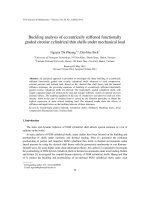
Figure 11 shows the effects of the elastic
foundations on the postbuckling behavior of FG
multilayer GPLRC plate. Elastic foundations are
recognized to have strong impact, as
demonstrated by curve (KW = 0, KG = 0) and

(KW=0.1Gpa/m, KG = 0.01Gpa.m), which show

that the ability of sustaining compression load
will increase if the effects of elastic foundations
enhance from (KW=0, KG = 0) to (KW=0.1Gpa/m,

KG = 0.01Gpa.m).

5. Conclusions

The postbuckling behavior of FG multilayer
GPLRC plate under mechanical and thermal
loads is investigated based on the FSDT. Some
remarkable results are listed following.

- The postbucking strength of pattern X is the
best, next is pattern U and the least pattern O.

- Elastic foundation models have a positive
influence on postbuckling curves, specifically
making postbucking strength decrease.

- Increasing the values of GPL weight
fraction makes postbucking strength capacity better.

- Effect of geometry and dimension of GPL
is also discussed and demonstrated through
illustrative numerical examples.

Acknowledgement

This research is funded by Vietnam National
Foundation for Science and Technology
Development (NAFOSTED) under grant
number 107.02-2018.04. The authors are
grateful for this support.

0 0.5 1 1.5 2

0
0.1
0.2
0.3
0.4
0.5
0.6
0.7

0/h

(GPa)

Perfect (=0.0)
Imperfect (=0.1)

GPL=0.5%, KG=0, KW=0

1: b

GPL/tGPL=10

2: b

GPL/tGPL=10
2

3: b

GPL/tGPL=10
3

4: b

GPL/tGPL=10
4

(1)
(2)

(4)

(3)

0 0.5 1 1.5 2

0
0.1
0.2
0.3
0.4
0.5
0.6
0.7

0/h

(GPa)

Perfect (=0.0)
Imperfect (=0.1)
1: a

GPL/bGPL=1

2: a

GPL/bGPL=10

3: a

GPL/bGPL=20

(1)

O-GPLRC: W

GPL=0.5%, KG=0, KW=0

(3)
(2)

0 0.5 1 1.5 2

0
0.2
0.4
0.6
0.8
1
1.2
1.4

W0/h

(GPa)

Perfect (=0.0)
Imperfect (=0.1)

O-GPLRC, WGPL=0.5%
K

W=0.1GPa/m,

G=0.01GPa.m

KW=0,KG=0
K

</div>
(13)<div class='page_container' data-page=13>

References

[1] K.S. Novoselov, A.K. Geim, S.V. Morozov, D.
Jiang, Y. Zhang, S.V. Dubonos, I.V. Grigorieva,
A. Firsov, Electric filed effect in atomically thin
carbon films, Science 306 (2004) 666–669.
10.1126/science.1102896.
[2] K.S. Novoselov, D. Jiang, F. Schedin, T.J. Booth,

V.V. Khotkevich, S.V. Morozov, A.K. Geim,
Two-dimensional atomic crystals, Proceedings of
the National Academy of Sciences of the United

States of America 102 (2005) 10451–10453.

[3] C.D. Reddy, S. Rajendran, K.M. Liew,

Equilibrium configuration and continuum elastic
properties of finite sized graphene,
Nanotechnology 17 (2006) 864-870. https://doi.
org/10.1088/0957-4484/17/3/042.

[4] C. Lee, X.D. Wei, J.W. Kysar, J. Hone,
Measurement of the elastic properties and
intrinsic strength of monolayer graphene, Science
321 (2008) 385–388.
science.1157996.

[5] F. Scarpa, S. Adhikari, A.S. Phani, Effective
elastic mechanical properties of single layer
graphene sheets, Nanotechnology 20 (2009)
065709.
065709.

[6] Y.X. Xu, W.J. Hong, H. Bai, C. Li, G.Q. Shi,
Strong and ductile poly(vinylalcohol)/graphene
oxide composite films with a layered structure,
Carbon 47 (2009) 3538–3543.
10.1016/j.carbon.2009.08.022.

[7] J.R. Potts, D.R. Dreyer, C.W. Bielawski, R.S.
Ruoff, Graphene-based polymer nanocomposites,
Polymer 52 (2011) 5-25.

.polymer.2010.11.042.

[8] T.K. Das, S. Prusty, Graphene-based polymer
composites and their applications,
Polymer-Plastics Technology and Engineering 52 (2013)
319-331.
751410.

[9] M. Song, J. Yang, S. Kitipornchai, W. Zhud,
Buckling and postbuckling of biaxially
compressed functionally graded multilayer
graphene nanoplatelet-reinforced polymer
composite plates, International Journal of
Mechanical Sciences 131–132 (2017) 345–355.

[10] H.S. Shen, Y. Xiang, F. Lin, D. Hui, Buckling and

postbuckling of functionally graded
graphene-reinforced composite laminated plates in thermal
environments, Composites Part B 119 (2017)
67-78.
03.020.

[11] H. Wu, S. Kitipornchai, J. Yang, Thermal
buckling and postbuckling of functionally graded
graphene nanocomposite plates, Materials and
Design 132 (2017) 430–441.
1016/j.matdes.2017.07.025.

[12] J. Yang, H. Wu, S. Kitipornchai, Buckling and

postbuckling of functionally graded multilayer
graphene platelet-reinforced composite beams,
Composite Structures 161 (2017) 111–118.

[13] H.S. Shen, Y. Xiang, Y. Fan, Postbuckling of

functionally graded graphene-reinforced
composite laminated cylindrical panels under
axial compression in thermal environments,
International Journal of Mechanical Sciences 135
(2018) 398–409.
csci.2017.11.031.

[14] M.D. Rasool, B. Kamran, Stability analysis of
multifunctional smart sandwich plates with
graphene nanocomposite and porous layers,
International Journal of Mechanical Sciences 167
(2019) 105283.
ci.2019.105283.

[15] J.J. Mao, W. Zhang, Buckling and post-buckling
analyses of functionally graded graphene
reinforced piezoelectric plate subjected to electric
potential and axial forces, Composite Structures
216 (2019) 392–405.
compstruct.2019.02.095.

[16] P.H. Cong, N.D. Duc, New approach to
investigate nonlinear dynamic response and
vibration of functionally graded multilayer

graphene nanocomposite plate on viscoelastic
Pasternak medium in thermal environment, Acta
Mechanica 229 (2018) 651-3670.
10.1007/s00707-018-2178-3.

[17] N.D. Duc, N.D. Lam, T.Q. Quan, P.M. Quang,
N.V. Quyen, Nonlinear post-buckling and
vibration of 2D penta-graphene composite plates,
Acta Mechanica (2019),
1007/s00707-019-02546-0.

[18] N.D. Duc, P.T. Lam, N.V. Quyen, V.D.
Quang, Nonlinear Dynamic Response and
Vibration of 2D Penta-graphene Composite
Plates Resting on Elastic Foundation in Thermal
Environments, VNU Journal of Science:
Mathematics-Physics 35(3) (2019) 13-29. https://
doi.org/10.25073/2588-1124/vnumap. 4371.
[19] J.N. Reddy, Mechanics of laminated composite

plates and shells; theory and analysis, Boca
Raton: CRC Press, 2004.

</div>


<a href=' /><a href=' /><a href=' /> Báo cáo khoa học: Absence of the psbH gene product destabilizes photosystem II complex and bicarbonate binding on its acceptor side in Synechocystis PCC 6803 ppt