EMISSION CONTROL (EMCON)
Bạn đang xem bản rút gọn của tài liệu. Xem và tải ngay bản đầy đủ của tài liệu tại đây (130.15 KB, 7 trang )
RF
System
-34 dBm (at RF port)
MIL-STD-461B/C RE-02 or
MIL-STD-461D RE-102
70 dBµV/m for externally mounted systems
= -110 dBm/m
2
1 Meter
1 Nautical mile
Seam or
Connector
Leakage
Maximum
EMCON
Emissions
(For Line Loss = Antenna Gain)
P G
t t
4BR
2
P
D
'
P
t
G
t
4BR
2
4-12.1
Figure 1. EMCON Field Intensity / Power Density Measurements
EMISSION CONTROL (EMCON)
When EMCON is imposed, RF emissions must not exceed -110 dBm/meter at one nautical mile. It is best if
2
systems meet EMCON when in either the Standby or Receive mode versus just the Standby mode (or OFF). If one assumes
antenna gain equals line loss, then emissions measured at the port of a system must not exceed -34 dBm (i.e. the stated
requirement at one nautical mile is converted to a measurement at the antenna of a point source - see Figure 1). If antenna
gain is greater than line loss (i.e. gain 6 dB, line loss 3 dB), then the -34 dBm value would be lowered by the difference and
would be -37 dBm for the example. The opposite would be true if antenna gain is less.
To compute the strength of emissions at the antenna port in Figure 1, we use the power density equation (see Section 4-2)
[1] or rearranging P G = P (4BR ) [2]
t t D
2
Given that P = -110 dBm/m = (10) mW/m , and R = 1 NM = 1852 meters.
D
2 -11 2
P G = P (4BR ) = (10 mW/m )(4B)(1852m) = 4.31(10) mW = -33.65 . -34 dBm at the RF system antenna as given.
t t D
2 -11 2 2 -4
or, the equation can be rewritten in Log form and each term multiplied by 10:
10log P + 10log G = 10log P + 10log (4BR ) [3]
t t D
2
Since the m terms on the right side of equation [3] cancel, then:
2
10log P + 10log G = -110 dBm + 76.35 dB = -33.65 dBm . -34 dBm as given in Figure 1.
t t
If MIL-STD-461B/C RE02 (or MIL-STD-461D RE-102) measurements (see Figure 2) are made on
seam/connector leakage of a system, emissions below 70 dBFV/meter which are measured at one meter will meet the
EMCON requirement. Note that the airframe provides attenuation so portions of systems mounted inside an aircraft that
measure 90 dBFV/meter will still meet EMCON if the airframe provides 20 dB of shielding (note that the requirement at
one nm is converted to what would be measured at one meter from a point source)
The narrowband emission limit shown in Figure 2 for RE02/RE102 primarily reflect special concern for local
oscillator leakage during EMCON as opposed to switching transients which would apply more to the broadband limit.
MIL-STD-461D RE-102 Navy/AF Internal
MIL-STD-461D RE-102 Army Int/Ext and Navy/AF External
MIL-STD-461B/C RE-02 AF and Navy Equipment
MIL-STD-461B/C RE-02 Army Equipment
P
D
'
P
t
G
t
4BR
2
4.37x10
&4
4B
mW/m
2
' .348x10
&4
mW/m
2
' &44.6 dBm/m
2
' P
D
E ' P
D
Z ' 3.48x10
&8
@ 377S ' 36.2x10
&4
V/m
4-12.2
Figure 2. MIL-STD-461 Narrowband Radiated Emissions Limits
Note that in MIL-STD-461D, the narrowband radiated emissions limits were retitled RE-102 from the previous
RE-02 and the upper frequency limit was raised from 10 GHz to 18 GHz. The majority of this section will continue to
reference RE02 since most systems in use today were built to MIL-STD-461B/C.
For the other calculation involving leakage (to obtain 70 dBFV/m) we again start with:
and use the previous fact that: 10log (P G ) = -33.6 dBm = 4.37x10 mW (see Section 2-4).
t t
-4
The measurement is at one meter so R = 1 m
2 2
we have: @ 1 meter
Using the field intensity and power density relations (see Section 4-1)
Changing to microvolts (1V = 10 FV) and converting to logs we have:
6
20 log (E) = 20 log (10 x 36.2x10 ) = 20 log (.362x10 ) = 71.18 dBFV/m . 70 dBFV/m as given in Figure 1.
6 -4 4
AF '
E
V
'
377 P
D
50 P
D
(8
2
G
r
/ 4B)
'
9.73
8 G
r
20 log AF ' 20logE & 20logV ' 20log
9.73
8 G
r
with 8 in meters and Gain numeric ratio (not dB)
4-12.3
[5]
[6]
Some words of Caution
A common error is to only use the one-way free space loss coefficient " directly from Figure 6, Section 4-3 to
1
calculate what the output power would be to achieve the EMCON limits at 1 NM. This is incorrect since the last term on
the right of equation [3] (10 Log(4BR )) is simply the Log of the surface area of a sphere - it is NOT the one-way free space
2
loss factor " . You cannot interchange power (watts or dBW) with power density (watts/m or dBW/m ).
1
2 2
The equation uses power density (P ), NOT received power (P ). It is independent of RF and therefore varies only
D r
with range. If the source is a transmitter and/or antenna, then the power-gain product (or EIRP) is easily measured and it's
readily apparent if 10log (P G ) is less than -34 dBm. If the output of the measurement system is connected to a power
t t
meter in place of the system transmission line and antenna, the -34 dBm value must be adjusted. The measurement on the
power meter (dBm) minus line loss (dB) plus antenna gain (dB) must not be higher than -34 dBm.
However, many sources of radiation are through leakage, or are otherwise inaccessible to direct measurement and
P must be measured with an antenna and a receiver. The measurements must be made at some RF(s), and received signal
D
strength is a function of the antenna used therefore measurements must be scaled with an appropriate correction factor to
obtain correct power density.
RE-02 Measurements
When RE-02 measurements are made, several different antennas are chosen dependent upon the frequency range
under consideration. The voltage measured at the output terminals of an antenna is not the actual field intensity due to actual
antenna gain, aperture characteristics, and loading effects. To account for this difference, the antenna factor is defined as:
AF = E/V [4]
where E = Unknown electric field to be determined in V/m ( or µV/m)
V = Voltage measured at the output terminals of the measuring antenna
For an antenna loaded by a 50 S line (receiver), the theoretical antenna factor is developed as follows:
P A = P = V /R = V /50 or V = o 50P A
D e r r r D e
2 2
ÕÕÕÕÕ
From Section 4-3 we see that A = G 8 /4B, and from Section 4-1, E = 377 P therefore we have:
e r D
2 2
Reducing this to decibel form we have:
This equation is plotted in Figure 3.
30 50 100 MHz 200 300 500 1 GHz 2 3 5 10 GHz 20 30
0
10
20
30
40
50
60
Radio Frequency
0
10
20
30
40
50
60
30 50 100 MHz 200 300 500 1 GHz 2 3 5 10 GHz 20 30
Prohibited
Region
Permissible
Region
4-12.4
Figure 3. Antenna Factor vs Frequency for Indicated Antenna Gain
Since all of the equations in this section were developed using far field antenna theory, use only the indicated region.
In practice the electric field is measured by attaching a field intensity meter or spectrum analyzer with a narrow
bandpass preselector filter to the measuring antenna, recording the actual reading in volts and applying the antenna factor.
20log E = 20log V + 20log AF [7]
Each of the antennas used for EMI measurements normally has a calibration sheet for both gain and antenna factor
over the frequency range that the antenna is expected to be used. Typical values are presented in Table 1.
Table 1. Typical Antenna Factor Values
Frequency Range Antenna(s) used Antenna Factor Gain(dB)
14 kHz - 30 MHz 41" rod 22-58 dB 0 - 2
20 MHz - 200 MHz Dipole or Biconical 0-18 dB 0 - 11
200 MHz - 1 GHz Conical Log Spiral 17-26 dB 0 - 15
1 GHz - 10 GHz Conical Log Spiral or Ridged Horn 21-48 dB 0 - 28
1 GHz - 18 GHz Double Ridged Horn 21-47 dB 0 - 32
18 GHz - 40 GHz Parabolic Dish 20-25 dB 27 - 35
AF '
E
V
'
377 P
D
50P
D
A
e
'
2.75
A
e
20logAF ' 20logE & 20logV ' 20log
2.75
A
e
System(s)
Under Test
Spectrum
Analyzer
Spiral
Antenna
25 ft
RG9 Cable
2 m
4-12.5
[8]
[9]
The antenna factor can also be developed in terms of the receiving antenna's effective area. This can be shown as follows:
Or in log form:
While this relation holds for any antenna, many antennas (spiral, dipole, conical etc.) which do not have a true
"frontal capture area" do not have a linear or logarithmic relation between area and gain and in that respect the parabolic
dish is unique in that the antenna factor does not vary with frequency, only with effective capture area. Consequently a
larger effective area results in a smaller antenna factor.
A calibrated antenna would be the first choice for making measurements, followed by use of a parabolic dish or
"standard gain" horn. A standard gain horn is one which was designed such that it closely follows the rules of thumb
regarding area/gain and has a constant antenna factor. If a calibrated antenna, parabolic dish, or "standard horn" is not
available, a good procedure is to utilize a flat spiral antenna (such as the AN/ALR-67 high band antennas). These antennas
typically have an average gain of 0 dB (typically -4 to +4 dB), consequently the antenna factor would not vary a lot and any
error would be small.
EXAMPLE:
Suppose that we want to make a very general estimation regarding the ability of a system to meet EMCON
requirements. We choose to use a spiral antenna for measurements and take one of our samples at 4 GHz. Since we know
the gain of the spiral is relatively flat at 4 GHz and has a gain value of approximately one (0 dB) in that frequency range.
The antenna is connected to a spectrum analyzer by 25 feet of RG9 cable. We want to take our measurements at 2 meters
from the system so our setup is shown below:
Our RG9 cable has an input impedance of 50S, and a loss of 5 dB (from Figure 5, Section 6-1).