Gis based land use simulation of sustainable forest management and wood utilization in thai nguyen province vietnam
Bạn đang xem bản rút gọn của tài liệu. Xem và tải ngay bản đầy đủ của tài liệu tại đây (13.71 MB, 209 trang )
GIS based Land use Simulation of Sustainable Forest
Management and Wood Utilization
in Thai Nguyen Province, Vietnam
Dissertation
With the aim of achieving a doctoral degree
At the Faculty of Mathematics, Informatics and Natural Sciences
Department of Biology
Of Universität Hamburg
Submitted by
Dang Cuong Nguyen
Hamburg, 2018
0
Day of oral defense: July, 5th 2018
The following evaluators recommended the admission of the dissertation
Supervisor: Prof.Dr. Michael Köhl
Co-supervisor: Prof.Dr. Gherardo Chirici
Chairman of examination committee: Prof. Dr. Jörg Fromm
I
Declaration
I hereby declare, under oath, that I have written the present dissertation on my
own and have not used any resources and aids other than those acknowledged.
…………………………………………………………….
Dang Cuong Nguyen
Hamburg, July 2018
II
English review testimonial
I certify that the English in the thesis:
GIS based Land use Simulation of Sustainable Forest Management and Wood
Utilization in Thai Nguyen Province, Vietnam
written by Dang Cuong Nguyen was reviewed and is correct.
Susan J. Ortloff (US citizen), freelance translator and editor
Susan J. Ortloff, July 10, 2017
III
Acknowledgement
During my doctoral studies at the Center for Wood Sciences, World Forestry and
the Department of Biology at the Universtät Hamburg, I received a great deal of
support from many people. I would like to express my deepest gratitude to my
supervisor Prof. Dr. Michael Köhl for his intellectual advice, encouragement and
valuable guidance. His valuable comments have been the most helpful in improving
this thesis. I am also thankful to Prof. Dr. Gherardo Chirici, Universita Degli Studi
Firenze for being my second supervisor.
I would like to express my sincere gratitude to Dr. Volker Mues for discussions,
suggestions and occasional technical support at various stages of this study from the
course of my fieldwork to the final dissertation. I am indebted to Dr. Prem Neupane
for introducing me to Prof. Dr. Köhl and the World Forestry Center in Hamburg.
Words are not sufficient to express my thanks to them.
I would like to sincerely thank the Ministry of Education and training of VietNam
(MoET) and Universtät Hamburg (Center for Wood Sciences, World Forestry) for
providing me with a scholarship during my studies in Germany and financial
support for fieldwork in Vietnam, respectively. Special thanks go to Konstantin
Olschofsky, Daniel Kübler, Dr.Timo Schönfeld, Dr.Philip Mundhenk, Laura Prill,
Vlad Strimbu and Giulio Di Lallo for their hospitality. They always stood by my
side and encouraged me.
My sincere thanks to Prof. Dr. Do Dinh Sam, Prof. Dr. Ngo Dinh Que, Dr. Nguyen
Thi Thu Hoan, and MA. Bach Tuan Dinh for their support and evaluations. In the
course of my fieldwork, I would like to thank Mr. Phan Trung Nghia and Mr.
Nguyen Anh Duc, key members of my research team, for their support during this
time. My sincere thanks to Mr. Khuong Van Khai, working in center for Marine
Hydro met research, Vietnam Institute of Meteorology, Hydrology and climate
change, for providing climate data. It was impossible to conduct this study without
contributions from Tran Ho who provided soil map and forest land cover map. I am
IV
obliged to the province forest officers, forest owners, and mills in the study area for
providing opportunities to collect useful information.
Special thanks go to Mrs. Doris Wöbb and Mrs. Sybille Wöbb for their
unconditional support in administrative issues and their caring assistance during my
stay in Germany. I am grateful to my wonderful colleagues at the Center for Wood
Sciences, World Forestry.
My loving thanks go to my wife Thi Thu Huong Nguyen and my son Dang Khoa
Nguyen for their patience, understanding, encouragement, and support during my
study abroad.
V
Research summary
The concept of Sustainable Forest Management (SFM) is well established. Its
principles of sustainable forest development and land use planning often require a
compromise between socio-economic development and environmental interests.
Biophysical factors have a significant effect on the productivity of forest
plantations, while socio-economical and economic factors impact profitability and
management systems. To enhance profits from forest plantations, the tree species
grown need to match the specific site conditions. At the same time, the efficiency of
forest plantations depends not only on forest site productivity, but also on market
driven factors such as timber price, timber demand and transportation cost..
This study uses a combination of a land suitability assessments based on FAO
framework for land suitability classification, multi-criteria, linear programming (LP)
and a Geographic Information System (GIS) framework to identify suitable
locations and achieve the highest profit for forest plantation management. A
suitability analysis and an optimization analysis were used. The suitability analysis
with classes highly suitable, moderately suitable, marginally suitable, and unsuitable
was conducted through a combination of land suitability assessments and multicriteria decision analysis (Analytic Hierarchy Process, AHP). Three main criteria
were used in the suitability analysis comprising soil properties, climate and
topography. Maps presenting suitability classes were established in ArcGIS
environment by Weighted Linear Combination (WLC). To reflect growth of the
studied species, volume growth was modeled using three models including
Chapman Richard, Gompert and Koft models. All three models reflected growth
well based on coefficient of determination (r2) and root mean square error (RMSE).
However, the Koft model performed best and was selected in the optimization
analysis to assign productivity on each suitability class.
The results of the suitability analysis were used in the optimization analysis. The
optimization model was built by combining programming (visual basic application
environment) and GIS (ArcGIS environment). The optimization model indicates
VI
that the optimal harvest age of a Acacia mangium plantation in the study area is 6
years, at which time the highest profits can be reached. The model used shows the
tradeoff between timber demand and timber supply. When timber demand increases,
profit obtained from forest plantations has a decreasing trend because of the
assignment of areas having lower profit due to lower productivity and higher costs.
The optimization model also illustrates that even considerably small variations in
timber price and costs have significant effects on the profit obtained and land area
allocated to respective mills.
The optimization model suggests the possibility of combining the needs of
environmental conservation with socio-economic demands of stakeholders by
establishing nature conservation areas. Shadow pricing can be used as a mean to
derive compensation payment to assign and maintain forest areas for protective use.
Additionally, the optimization model provides a tool to study the establishment of
co-operated mills. Three new mills could replace 215 existing mills and 3 new mills
could be added with higher capacities.
The findings of this study provide evidence for the need of a concurrent forest land
utilization and mill development planning in order to maintain and enhance
economic and ecological objectives and to improve local livelihoods. This holds
especially true under extensive afforestation and reforestation activities, as recently
promoted by the Bonn Challenge and the New York Declaration.
VII
Content
Research summary
VI
Content
VIII
List of tables
XII
List of figures
XIV
List of abbreviations
XIX
1
Introduction
1.1
The demand and supply wood from planted forest
1
1.2
The role of forestry in the Vietnam economy
6
1.3
Forest cover and plantations in Vietnam
8
1.4
The problem statement
12
1.5
Research question and objectives
16
1.5.1
Research questions
16
1.5.2
Research objectives
16
1.6
2
1
The structure of thesis
17
Literature review
18
2.1 Application of the FAO framework and multi-criteria decision analysis in
land suitability assessment
18
2.1.1
FAO framework
18
2.1.2
Multiple criteria decision making
21
2.2
3
Application of linear programming in land use suitability analysis
Material and methodology
3.1
26
31
Materials
31
3.1.1
Study area
31
3.1.2
Studied species
34
VIII
3.1.3
3.2
Data sources as basis for suitability mapping
38
3.1.3.1 Soil properties
38
3.1.3.2 Climate
40
3.1.3.3 Topography
41
Methods
3.2.1
42
Modelling suitability
42
3.2.1.1 Determination of ecological factors and classes for each ecological
factor 43
3.2.1.2 Determination score assignment to suitability classes and weight for
ecological factor
44
3.2.1.3 Land suitability integration by weighted linear combination
3.2.2
48
3.2.2.1 Technical equipment for execution of inventory on growth
48
3.2.2.2 Selection of stands for forest measurement
48
3.2.2.3 Design and location of sample plot
52
3.2.2.4 Calculation of stand variables
54
3.2.2.5 Adjustment of sample area at forest edges
55
3.2.2.6 Modelling volume growth for suitability classes
56
3.2.3
Determination of optimal rotation as maximum sustained yield
3.2.4
Assessment of socio-economic aspects of Acacia mangium plantations
58
3.2.5
Scenario simulation with geo-explicit optimization methods
57
61
3.2.5.1 Geo-explicit optimization model
61
3.2.5.2 Calculation of transportation cost in ArcGIS environment
67
3.2.6
4
Modelling productivity
47
Scenario analysis
69
Results
72
IX
4.1
Results of questionnaire
72
4.1.1
Result of questionnaires on forest activities of households
72
4.1.2
Results of questionnaires on sawmills
76
4.1.3
Assignment of suitability classes for Acacia mangium
78
4.2
Growth of Acacia mangium
83
4.2.1
Number of trees per hectare – diameter classes distribution according
to suitability classes
83
4.2.2
Stand variables according to suitability classes
88
4.2.3
Growth function
91
4.3
Scenario results
4.3.1
BAU (Business As Usual)
4.3.2
Rotation ages
100
4.3.3
ECO (economic scenario)
104
95
4.3.3.1 ECO_demand
104
4.3.3.2 ECO_ price
120
4.3.3.3 ECO_ cost
129
4.3.4
Mill_new and Mill_coop
136
4.3.4.1 Mill_new
136
4.3.4.2 Mill_coop
139
4.3.5
5
95
Nature conservation area
144
Discussion
5.1
150
Discussion of suitability and growth model
150
5.1.1
Land suitability assessment
150
5.1.2
Forest growth model and productivity
152
5.2
Profitability maximization from growing forest plantations
X
153
6
5.2.1
Optimal rotation age
153
5.2.2
Profitability maximization from growing plantation
154
Conclusion
158
References
160
Appendix
175
XI
List of tables
Table 1.1 Area of planted forest by region from 1990 to 2010 ................................... 3
Table 1.2 Predicted change in wood volume produced in planted forests between
2005 and 2030 (million m3 year-1) .............................................................................. 4
Table 1.3 The change in forest cover for the period 1995 -2014 ................................ 8
Table 1.4 The planted forest area ................................................................................ 9
Table 2.1 Land suitability classes (FAO 1984) .........................................................19
Table 2.2 Scale for pairwise comparison (The Saaty fundamental 9-point scale) ....22
Table 3.1 Forested area according to forest types .....................................................33
Table 3.2 The information of soil properties.............................................................39
Table 3.3 The weather stations in study area ............................................................40
Table 3.4 The locations of 11 stations in which rainfall regime is collected ............40
Table 3.5 Random Index (Saaty 1980a) ....................................................................46
Table 4.1 Descriptive statistics on the size and spatial situation of the household
questionnaire (Exchange rate: 1 USD = 22000 VND) ..............................................73
Table 4.2 Characteristics of mills derived from the questionnaires ..........................76
Table 4.3 Parameters for determining suitable classes by experts ............................79
Table 4.4 Matrix of pair-wise comparison of all attributes by forestry experts ........79
Table 4.5 Weights of ecological parameters in land suitability assessment .............80
Table 4.6 Land suitability class for Acacia mangium ...............................................81
Table 4.7 Summary results of calculation of stand variables ....................................88
Table 4.8 The fitted models for tested species ..........................................................91
Table 4.9 Value selected for attributes in the optimization model............................96
Table 4.10 The results for the Landscape Approach and the Current Forest
Approach (PA: pallet mills, VE: veneer mills, WC: woodchip mills) ......................97
XII
Table 4.11 Land area allocated for the Landscape Approach and the Current Forest
Approach for harvesting A. mangium plantation at age 6 years..............................101
Table 4.12 Total forested area allocated in different timber demand amount over 6
years in the Current Forest Approach (_FO) ...........................................................106
Table 4.13 Change of profit with various timber demands for specific mill types
under the Landscape Approach, 6 – year rotation ...................................................111
Table 4.14 Change of profit with various timber demands for specific mill types
under the Current Forest Approach, 6 – year rotation.............................................112
Table 4.15 The timber price at mill types varied according sub-regions ................122
Table 4.16 Differences in cost, profit and land area allocated for growing plantations
with variations in timber price on 6-year-rotation ..................................................123
Table 4.17 Costs, profit and area varied by change of cost on 6 years rotation......131
Table 4.18 Distribution of timber demand and timber price at mills ......................136
Table 4.19 Different costs, profits and land area allocated for growing plantations by
adding new mills on 6-year rotation ........................................................................137
Table 4.20 Distribution of timber demand and price at mills .................................140
Table 4.21 Different costs, profits and land area needed by taking into consideration
larger mills on 6-year-rotation.................................................................................141
Table 4.22 The difference of total profit obtained between the basic timber demand
and increase of 20% ................................................................................................146
XIII
List of figures
Figure 1.1 Trend in area of planted forest between 1990 and 2010 (source: FAO
2010a) .......................................................................................................................... 1
Figure 1.2 Planted forest area by climate domain (Source: FAO 2015b) ................... 2
Figure 1.3 The trend in planted forest area from 1990 to 2015 in 20 countries
(Source: Payn et al. 2015) ........................................................................................... 5
Figure 1.4 Wood production export turnover varied in the period 2004 - 2011
(MARD 2014b) ........................................................................................................... 6
Figure 1.5 Wood production import turnover varied in the period 2006 - 2012
(MARD 2014b) ........................................................................................................... 7
Figure 1.6 The distribution of planted forest areas by region in Vietnam ................10
Figure 3.1 Location of study area..............................................................................32
Figure 3.2 Acacia mangium planted in 1 year old (a); 2 years old (b); 3 years old (c);
4 years old ( (d); 5 years old ( (e); 6 years old (f); 8 years old (g); 9 years old (h)
...................................................................................................................................37
Figure 3.3 Maps of soil types and soil depth in study area .......................................38
Figure 3.4 Mean annual precipitation map................................................................41
Figure 3.5 Elevation and slope gradient maps ..........................................................42
Figure 3.6 Research method for building a preliminary suitable site and potential
productivity map for forest plantations (AHP: Analytical Hierarchy Process, WLC:
weighted linear combination) ....................................................................................43
Figure 3.7 Hierarchical structure in the analytical hierarchy process .......................45
Figure 3.8 Discussion with a forestry expert (Do Dinh Sam) for AHP ....................47
Figure 3.9 Sketch of selecting alternative stand from selected stand........................49
Figure 3.10 Map showing forest functions and selected sample points distribution 51
Figure 3.11 Creating scheme for concentric plot ......................................................52
Figure 3.12 RD Criterion 1000 instrument (Source: ) .....53
XIV
Figure 3.13 Regulation of measurement of DBH (Source: Köhl et al. 2006) ...........54
Figure 3.14 Using GPS and diameter caliper in a forest survey ...............................55
Figure 3.15 Calculate the segment area given the radius and segment's central angle
...................................................................................................................................56
Figure 3.16 Transport of timber from forest (a, b, c), interviewing local household
(d), woodchip mill (e), veneer mill (f), Pallet mill (g, h) ..........................................60
Figure 3.17 Framework of an optimization model....................................................62
Figure 3.18 Map showing only the locations of land planned for production forest
including planted forest and un-planted forest areas .................................................63
Figure 3.19 New roads were built to be accessible to timber delivered (a, b) ..........67
Figure 3.20 Difference between straight line distance and transportation distance ..68
Figure 4.1 Planting density of A.mangium in Thai Nguyen province .......................73
Figure 4.2 Establishment cost and silviculture cost derived from questionnaire ......74
Figure 4.3 Stumpage price and harvest cost derived from questionnaire .................75
Figure 4.4 Different timber prices at mills according to mill types ..........................77
Figure 4.5 Different timber demands according to mill types ..................................77
Figure 4.6 Map of suitability locations for growing A. mangium .............................82
Figure 4.7 Distribution of number of trees (S1: 14 plots, S2: 12 plots, S3: 5 plots,
calculated per hectare) in different suitability classes. a) Absolute number of trees
and b) Relative number of trees according to diameter classes ................................84
Figure 4.8 Distribution of number of trees (S1: 29 plots, S2: 31 plots, S3: 25 plots,
calculated per hectare) in different suitability classes. a) Absolute number of trees
and b) Relative number of trees according to diameter classes ................................85
Figure 4.9 Distribution of number of trees (S1: 14 plots, S2: 17 plots, S3: 3 plots,
calculated per hectare) in different suitability classes. a) Absolute number of trees
and b) Relative number of trees according to diameter classes ................................86
Figure 4.10 Distribution of number of trees (S1: 4 plots, S2: 11 plots, S3: 12 plots,
calculated per hectare) in different suitability classes. a) Absolute number of trees
and b) Relative number of trees according to diameter classes ................................87
XV
Figure 4.11 Relationship between quadratic mean diameter and number of tree per
hectare in different suitability classes .......................................................................89
Figure 4.12 Distribution of volume per hectare over age by different suitability
classes ........................................................................................................................90
Figure 4.13 Volume growth curves for tested species in three suitability classes (a:
S; b: S2, c: S3) growth functions for the suitability classes (d) ................................92
Figure 4.14 Biological optimum to gain the maximization of the sustainable yield
(CAI: current annual increment, MAI: Mean annual increment), (S1: highly
suitable, S2: Moderately suitable, S3: Marginally suitable) .....................................93
Figure 4.15 Map showing productivity for A. mangium plantations at age 6 years on
the land area planned for production forest ...............................................................94
Figure 4.16 Difference in cost components for the _LA approach and the _FO
approach ....................................................................................................................98
Figure 4.17 Maps showing land area allocated under the Landscape Approach
(_LA) and the Current Forest Approach (_FO) for Acacia mangium at age 7 years 99
Figure 4.18 Profit per hectare by age for A. mangium plantations..........................100
Figure 4.19 Profit per hectare per year by age for A.mangium plantation ..............101
Figure 4.20 Maps showing land area allocated under the Landscape Approach
(_LA) and the Current Forested Approach (_FO) for Acacia mangium at age 6 years
.................................................................................................................................103
Figure 4.21 Difference in household profit achieved by the Landscape Approach
and the Current Forest Approach according to variations in timber demand .........105
Figure 4.22 The effect of timber demand on profit/m3 and transportation cost/m3108
Figure 4.23 Change in costs in the Landscape Approach (a) and the Current Forest
Approach (b) based on timber demand variations ..................................................109
Figure 4.24 Change in profit per hectare for the Landscape Approach (blue color)
and the Current Forest Approach (red color) when timber demand is changed for
specific mill types....................................................................................................113
Figure 4.25 Maps showing the distribution of land area allocated by decreasing
timber demand 30% on 6 – year rotation ................................................................115
XVI
Figure 4.26 Maps showing the distribution of land area allocated by increasing
timber demand 20% on 6 – year rotation ................................................................116
Figure 4.27 Maps showing the distribution of land area allocated by increasing 30%
timber demand on 6 – year rotation ........................................................................117
Figure 4.28 Maps showing the distribution of land area allocated by increasing
timber demand 40% on 6 – year rotation ................................................................118
Figure 4.29 Maps showing the distribution of land area allocated by increasing
timber demand 50% on 6 – year rotation ................................................................119
Figure 4.30 Map showing various timber prices at mills ........................................120
Figure 4.31 Profit per hectare obtained by timber prices at mills on 6 – year rotation
.................................................................................................................................124
Figure 4.32 Transportation cost varied according to timber price for the Landscape
Approach and the Current Forest Approach ...........................................................124
Figure 4.33 Maps showing the distribution of land area allocated by variations in
timber price according to sub-regions on 6 – year rotation.....................................125
Figure 4.34 Maps showing the distribution of land area allocated by assumption of
equal timber price 52.3$/m3 to mills on 6 – year rotation .......................................126
Figure 4.35 Maps showing the distribution of land area allocated by assumption of
equal timber price 53.6$/m3 to mills on 6 – year rotation .......................................127
Figure 4.36 Maps shows the distribution of land area allocated by assumption of
equal timber price of 55.6$/m3 to mills on 6 – year rotation ..................................128
Figure 4.37 Distribution of harvest cost in different altitude ..................................130
Figure 4.38 Distribution of applied silviculture cost in different altitude ...............130
Figure 4.39 Maps showing the distribution of land area allocated by assumption of
siviculture cost change on 6 – year rotation ............................................................133
Figure 4.40 Maps showing the distribution of land area allocated by assumption of
harvest cost change on 6 – year rotation .................................................................134
Figure 4.41 Maps showing the distribution of land area allocated by concurrent
changes of silviculture and harvest costs on 6 years rotation .................................135
Figure 4.42 Maps showing land area allocated by adding 3 new mills ..................138
XVII
Figure 4.43 Replacement of 215 existing mills by 24 larger mills .........................139
Figure 4.44 Maps showing a difference of in land allocated to mills between the
Mill_coop scenario and ROT_6 scenario for the Landscape Approach .................142
Figure 4.45 Maps showing a difference in land allocated to mills between Mill_coop
scenario and ROT_6 scenario for the Current Forest Approach .............................143
Figure 4.46 Maps showing 5 locations considered as nature conservation areas ...145
Figure 4.47 Map showing a possible solution to form nature conservation areas in
remote area ..............................................................................................................147
Figure 4.48 Maps showing land area allocated to mills considering nature
conservation under usual timber demand ................................................................148
Figure 4.49 Maps showing land area allocated to mills when considering nature
conservation by increasing timber demand by 20%................................................149
XVIII
List of abbreviations
5MHRP
The Five Million Hectare Reforestation Program
AHP
Analytic hierarchy process
AIJ
Aggregation of individual judgments
AIP
Aggregation of individual priorities
CAI
Current Annual Increment
CFS-AFM
Canadian Forest Service – Afforestation Feasibility Model
CI
Consistency index
CR
Consistency ratio
DBH
Diameter at Breast Height
Dg
Quadratic mean diameter
DEM
Digital elevation model
FAO
Food and Agriculture Organization of the United Nations
FO
Current forest approach
FIPI
Forest Inventory and Planning Institute
GDP
Gross Domestic Product
GIS
Geographic Information System
GPS
Global Position System
GSO
General Statistics Office
Ha
Hectare
IDW
Inverse Distance Weighted
LA
Landscape approach
LEV
Land expectation value
LP
Linear programming
MAI
Mean Annual Increment
XIX
MARD
Development of the Ministry of Agriculture and Rural
Development
MCDA
Multiple Criteria Decision Analysis
NYDF
New York Declaration on Forest
NPV
Net Present Value
PA
Pallet
PCT
People’s committee Thai Nguyen
R2
Coefficient of determination
RI
Random index
RMSE
Root mean square error
SUF
Special Use Forest
SRTM
Shuttle Radar Topographic Mission
SWOT
Strength, Weaknesses, Opportunities, Threats
UNESCO
United Nations Educational, Scientific and Cultural
Organization
USD
United States Dollar
VAAS
Vietnam Academy of Agricultural Sciences
VE
Veneer
VN2000
Vietnam coordinate projection
WC
Woodchip
WLC
Weighted Linear Combination
XX
1
Introduction
1.1 The demand and supply wood from planted forest
A forest plantation is defined as “forest stands established through planting or seeding of one
or more indigenous or introduced tree species by afforestation or reforestation programs,
which demands a series of criteria: one or two species at planting, even age class, and regular
spacing” (FAO 2006). The main aim of forest plantations is to provide wood supply as timber,
fiber, fuel wood or bioenergy, non-wood forest products (FAO 2015b). Planted forests
provided about 35% of the global wood supply in 2000 (Brockerhoff et al. 2008), and 46.3%
of industrial roundwood in 2012 (Payn et al. 2015).
Figure 1.1 Trend in area of planted forest between 1990 and 2010 (source: FAO 2010a)
Due to the rapid growth in forest plantations, they have been able to meet the increasing
global demand for timber, fuel and fiber. The total planted forest area increased by around 5
million hectares per year from 2000 to 2010, amounting to 264 million hectares in 2010 and
estimated to reach 300 million hectares in the near future (FAO 2010b). The average annual
amount of planted area increased more slowly between 2010 and 2015, by around 3.1 million
1
hectares, than in the period between 2000 to 2010 (FAO 2015b). Most of the planted forests
were established through afforestation programs (FAO 2010a).
Figure 1.2 Planted forest area by climate domain (Source: FAO 2015b)
Figure 1.2 shows that the planted area continuously increased from 1990 to 2015, increasing
its share in the global forest area from 4.1% to 7% (FAO 2015b). The largest area belongs to
the temperate zone, followed by the Boreal and tropical zone, and the smallest area to the
subtropical zone. Estimation of the future supply and demand for wood and wood products
are an important aid to planning and decision making in the forestry sector at a national,
regional and global level (FAO 1999). The global production of all major wood products
including roundwood, sawnwood, wood-based panels, pulp and paper increased in 2013
compared with 2009. For instance, the paper and paperboard production increased from 371
million tons in 2009 to 398 million tons in 2013 (FAO 2013). The rise in the global human
population, sustained economic growth, regional shifts, regulations and energy policies are
2
the main reasons for the change in the long term global demand for wood products; along
with a decline in harvesting from natural forests. This places a significant pressure on the
global forest to use planted forests to meet the demand for wood products (FAO 2009a, 2012).
As demand for forest products grows, and natural forests are increasingly degraded and
decreased in size, the total area of forest land has remained unchanged (FAO 2010a, 2015b).
Natural forests have declined by 6.6 million hectares per year from 2010 to 2015 and the trend
is predicted to continue in the future. This has increased the demand on planted forests to
supply forest products. Consequently, commercial forest plantations are increasingly
replacing natural forests as a timber source (Heilmayr 2014), accounting for 26% (816 million
m3) of the global timber harvest (Buongiorno and Zhu 2014).
The amount of planted forest area worldwide significantly increased in the period 1990 to
2010, as shown below in Table 1.1.
Table 1.1 Area of planted forest by region from 1990 to 2010
Area of planted forest (1000 ha)
Region
Annual increment (%)
1990
2000
2005
2010
19902000
20002005
20052010
Africa
1158
0
12873
14032
15326
1.1
1.7
1.8
Asia
7087
3
92871
109670
12277
7
2.7
3.4
2.3
Europe
5816
6
65309
68500
69318
1.2
1.0
0.2
NorthCentral
America
2005
6
30186
35786
38659
4.2
3.5
1.6
Oceania
2542
3322
3849
4100
2.7
3.0
1.3
South
America
8115
10058
11123
13821
2.2
2.0
4.4
Source: Borges et al. (2014)
3
The largest area of planted forest was found in the Asia, but the highest annual rate of change
in area belonged to South America in the period 2005 to 2010.
In a report on the state of the world’s forest to the year 2030, one scenario mentioned is an
annual productivity increase in wood supply from planted forests. An estimation of the
amount of wood supplied from planted forests in 2030 compared with 2005 shows that the
global volume produced in planted areas will increase from 1.4 billion m3 in 2005 to 1.7
billion m3 in 2030, as shown in Table 1.2.
Table 1.2 Predicted change in wood volume produced in planted forests between 2005 and
2030 (million m3 year-1)
Fuel/bioenergy
Pulp/fiber
Wood products
Region
2005
2030
2005
2030
2005
2030
Africa
11
10
9
15
55
56
Asia
79
88
141
146
264
321
Europe
17
18
123
129
166
185
3
6
26
55
26
56
7
8
98
117
24
31
19
23
133
173
91
115
Oceania
1
1
11
13
31
36
Total
136
155
540
647
659
800
Southern
Europe
America
South
America
Source: Borges et al. (2014)
4