Textbook of engineering drawing (2nd edition): Part 1

Bạn đang xem bản rút gọn của tài liệu. Xem và tải ngay bản đầy đủ của tài liệu tại đây (5.83 MB, 189 trang )

(1)<div class='page_container' data-page=1></div>
(2)<div class='page_container' data-page=2>

Textbook of

Engineering Drawing

Second Edition

K. Venkata Reddy

Prof. & HOD of Mechanical Engineering Dept.
C.R. Engineering College,

Tirupati - 517 506

SSP BS

Publications

;;;::::;;;;; 4-4-309, Giriraj Lane, Sultan Bazar,

</div>
(3)<div class='page_container' data-page=3>

Copyright © 2008, by Publisher 
AIl rights reserved

No part of this book or parts thereof may be reproduced, stored in a retrieval system or I
transmitted in any language or by any means, electronic, mechanical, photocopying,

I

iL

recording or otherwise without the prior written permission of the publishers. ~

Published by :

BSP BS Publications

===

4-4-309, Giriraj Lane, Sultan Bazar,

Hyderabad - 500 095 - A.P.
Phone: 040-23445688

Printed at

e-mail: 
www.bspublications.net

Adithya Art Printers

Hyderabad

</div>
(4)<div class='page_container' data-page=4>

Contents

CHAPTER-1

Drawing Instruments and Accessories

1.1-1.5

1.1 Introduction, 1.1

1.2 Role of Engineering Drawing, 1.1

1.3 Drawing Instrument and Aids, 1.1

1.3.1 Drawing Board, 1.2

1.3.2 Mini-Draughter, 1.2

1.3.3 Instrument Box, 1.2

1.3.4 Set of Scales, 1.3

1.3.5 French Curves, 1.4

1.3.6 Templates, 1.4

1.3.7 Pencils, 1.4

CHAPTER-

2

Lettering and Dimensioning Practices

2.1-2.25

2.1 Introduction. 2.1

2.2 Drawing Sheet, 2.1

2.2.1 Title Block, 2.2

2.2.2 Drawing Sheet Layout (Is 10711 : 2001), 2.3

2.2.3 Folding of Drawing Sheets, 2.3

</div>
(5)<div class='page_container' data-page=5>

COli/ellis

2.3 LETTERING [IS 9609 (PART 0) : 2001 AND S~ 46: 2003], 2.7

2.3.1 Importance of Lettering, 2.7

2.3.2 Single Stroke Letters, 2.7

2.3.3 Types of Single Stroke Letters, 2.7

2.3.4 Size of Letters, 2.8

2.3.5 Procedure for Lettering, 2.8

2.3.6 Dimensioning of Type B Letters, 2.8

2.3.7 Lettering Practice, 2.9

2.4 Dimensioning, 2.12

2.4.1 Principles of Dimensioning, 2.13

2.4.2 Execution of Dimensions, 2.15

2.4.3 Methods ofIndicating Dimensions, 2.17

2.4.4 IdentificatiollofShapes, 2.18

2.5 Arrangement of Dimensions, 2.19

CHAPTER-

3

Scales

3.1-3.12

3.1 Introduction, 3.1

3.2 Reducing and Enlarging Scales, 3.1

3.3 Representative Fraction, 3.2

3.4 Types of Scales, 3.2

3.4.1 Plain Scales, 3.2

3.4.2 Diagonal Scales, 3.5

3.4.3 Vernier Scales, 3.9

CHAPTER-4

Geometrical Constructions

4.1-4.51

4.1 Introduction, 4.1

4.2 Conic Sections 4.12

4.2.1 Circle, 4.13

4.2.2 Ellipse, 4.13

4.2.3 Parabola, 4.13

4.2.4 Hyperbola, 4.13

</div>
(6)<div class='page_container' data-page=6>

COll1ellts

4.3 Special Curves, 4.27
4.3.1 Cycloid,4.27

4.3.2 Epi-Cycloid and Hypo-Cycloid, 4.28
4.4 Involutes, 4.30

CHAPTER-

5

Orthographic Projections

5.1-5.35

5.1 Introduction, 5.1

5.2 Types of Projections, 5.2

5.2.1 Method ofObtaning, 5.2

5.2.2 Method ofObtaning Top View, 5.:?
5.3 FirstAngle Projectiom, 5.5

5.4 ThirdAngle Projection, 5.5
5.5 Projection of Points, 5.6
5.6 Projection of Lines, 5.13
5.7 Projection of Planes, 5.19

CHAPTER -

6

Projection of Solids

6.1-6.50

6.1 Introduction, 6.1

6.1.2 Polyhedra, 6.1

6.1.3 Regular of Polyhedra, 6.1
6.2 Prisms, 6.2

6.3 Pyramids, 6.3

6.4 Solids of Revolution, 6.3

6.5 Frustums of Truncated Solids, 6.3
6.6 Prims (Problem) Position of a

Solid with Respect to the Reference Planes, 6.4
6.7 Pyramids, 6.17

</div>
(7)<div class='page_container' data-page=7>

(xiv) COlltellts

6.9 Application ofOlthographic Projections, 6.30

6.9.1 Selection of Views, 6.30

6.9.2 Simple Solids, 6.30

6.9.3 Three View Drawings, 6.31

6.9.4 Development ofMissiong Views, 6.31

6.10 Types of Auxiliary Views, 6.45

CHAPTER-7

Development of Surfaces

CHAPTER-8

7.1 Introduction, 7.1

7.2 Methods of Development, 7.1

7.2.1 Develop[ment of Prism, 7.2

7.2.2 Development ofa Cylinder, 7.2

7.2.3 Development ofa square pyramid with side of

base 30 mm and height 60 mm, 7.3

7.2.4 Development of a Cone, 7.5

I ntersection of Surfaces

8.1 Introduction, 8.1

8.2 Intersection of cylinder and cylinder, 8.1

8.3 Intersection of prism and prism, 8.4

CHAPTER-9

Isometric Projection

9.1 Introduction, 9.1

9.2 Principle ofIsometric Projections, 9.1

9.2.1 Lines in Isometric Projection, 9.3

·9.2.2 Isometric Projection, 9.3

9.2.3 Isometric Drawing, 9.4

9.2.4 Non-Isometric Lines, 9.6

7.1-7.21

8.1-8.5

</div>
(8)<div class='page_container' data-page=8>

COlltellts (xv)

9.3 Methods of Constructing Isometric Drawing, 9.6

9.3.1 Box Method, 9.7

9.3.2 Off-set Method, 9.7

9.4 Isometric Projection of Planes, 9.7

9.5 Isometric Projection of Prisms, 9.13

9.6 Isometric Projection of Cylinder, 9.15

9.7 Isometric Projection of Pyramid, 9.15

9.8 Isometric Projection of Cone, 9.16

9.9 Isometric Projectin Truncated Cone, 9.17

CHAPTER-10

Oblique and Persepctive Projections

10.1-10.23

10.1 Introduction, 10.1

10.2 Oblique Projection, 10.1

10.3 Classification of Oblique Projection, 10.2

10.4 Methods of Drawing Oblique Projection 10.2

10.4.1 Choice of Position of the Object, 10.3

10.4.2 Angles, Circles and Curves in Oblique Projection 10.3

10.5 Perspective Projection, 10.5

10.5.1 Nomenclature of Perspective Projection, 10.6

10.5.2 Classification of perspective projections, 10.8

10.5.3 Methods of Perspective Projection, 10.10

CHAPTER-11

Conversion of Isometric Views to

Orthographic Views and Vice Versa

11.1 Introduction, 11.1

11.2 Selection of views, 11.1

11.1-11.8

</div>
(9)<div class='page_container' data-page=9>

(xvi)

CHAPTER-12

Sections of Solids

12.1 Sectioning of Solids, 12.1

12.1.1 Introduction, 12.1

12.1.2 Types of Section Views, 12.1

12.1.3 Cutting Plane, 12.1

CHAPTER-13

Freehand Sketching

13.1 Introduction, 13.1

CHAPTER-14

Computer Aided Design and

Drawing (CADD)

14.1 Introduction, 14.1

14.2 History of CAD, 14.1

14.3 Advantages of CAD, 14.1

14.4 Auto Cad Main Window, 14.2

14.4.1 Starting a New Drawing, 14.2

14.4.2 Opening an Existing Drawing, 14.3

14.4.3 Setting drawing limits, 14.4

14.4.4 Erasing Objects, 14.4

14.4.5 Saving a Drawing File, 14.4

14.4.6 Exiting an AutoCAD Session, 14.4

14.5.2 Polar Coordinates, 14.5

14.5 The Coordinate System, 14.5

14.5.1 Cartesian Coordinates, 14.5

14.6 The Fonnats to Enter Coordinates, 14.6

14.6.1 User-Defined Coordinate System, 14.6

COlltellts

12.1-12.13

13.1-13.6

</div>
(10)<div class='page_container' data-page=10>

COlltellls

14.7 Choosing Commands in AutoCAD, 14.8

14.7.1 Pull-down Menus [pd menu](Fig 14.6), 14.8
14.7.2 Tool Bar Selection, 14.9

14.7J Activating Tool Bars, 14.9
14.8 Right Mouse Clicking, 14.10

14.8.1 Right Mouse Click Menus, 14.11
14.9 Object Snaps, 14.12

14.9.1 Types of Object Snaps, 14.12
14.9.2

14.9J
14.9.4
14.9.5
14.9.6
14.9.7
14.9.8

14.9.9
14.9.10

Running Object Snaps, 14.13

Dividing an Object into Equal Segments, 14.14
Setting off Equal Distances, 14.14

Polyline Command, 14.14
Ray Command, 14.15
Rectangle Command, 14.15
Arc Command, 14. 15
Circle Command, 14.18
Ellipse Command, 14.19
14.10 The Drawing Tools of CADD, 14.20

14.10.1 Using Line Types, 14.20

14.10.2 Drawing Multiple Parallel Lines, 14.21
14.10J Drawing Flexible Curves, 14.21

14.10.4 Drawing Ellipses and Elliptical Arcs, 14.22

</div>
(11)<div class='page_container' data-page=11></div>
(12)<div class='page_container' data-page=12>

CHAPTER

1

1.1 Introduction

Drawing Instruments and

Accessories

Engineering drawing is a two dimensional representation of three dimensional objects. In general, it
provides necessary information about the shape, size, surface quality, material, manufacturing process,
etc., of the object. It is the graphic language from which a trained person can visualise objects.

Drawings prepared in one country may be utilised in any other country irrespective of the
language spoken. Hence, engineering drawing is called the universal language of engineers. Any
language to be communicative, should follow certain rules so that it conveys the same meaning to
every one. Similarly, drawing practice must follow certain rules, if it is to serve as a means of
communication. For this purpose, Bureau of Indian Standards (BIS) adapted the International
Standards on code of practice for drawing. The other foreign standards are: DIN of Germany, BS
of Britain and ANSI of America.

1.2 Role

of Engineering

Drawing

The ability to read drawing is the most important requirement of all technical people in any profession.
As compared to verbal or written description, this method is brief and more clear. Some of the
applications are : building drawing for civil engineers, machine drawing for mechanical engineers,
circuit diagrams for electrical and electronics engineers, computer graphics for one and all.

The subject in general is designed to impart the following skills.
1. Ability to read and prepare engineering drawings.
2. Ability to make free - hand sketching of objects.
3. Power to imagine, analyse and communicate, and
4. Capacity to understand other subjects:

1.3 Drawing Instrument and Aids

</div>
(13)<div class='page_container' data-page=13>

1.2 Textbook of Enginnering D r a w i n g

-1.3.1 Drawing Board

Until recently drawing boards used are made of well seasoned softwood of about 25 mm thick with
a working edge for T-square. Nowadays mini-draughters are used instead of T-squares which
can be fixed on any board. The standard size of board depends on the size of drawing sheet size
required.

r - - -Drawing board

Angle

Drawing sheet
Fig. 1.1 Mini-draughter

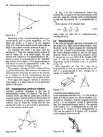
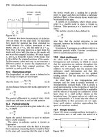
1.3.2 Mini-Draughter

Mini-draughter consists of an angle formed by two arms with scales marked and rigidly hinged to
each other (Fig. I. I ). It combines the functions ofT-square, set-squares, scales and protractor. It is
used for drawing horizontal, vertical and inclined lines, parallel and perpendicular lines and for
measuring lines and angles.

1.3.3 Instrument Box

Instrument box contains 1. Compasses, 2. Dividers and 3. Inking pens. What is important is the
position of the pencil lead with respect to the tip of the compass. It should be atleast I mm above as
shown in Fig. 1.2 because the tip goes into the board for grip by 1 mm.

(a) Sharpening and position of
compass lead

Fig. 1.2

</div>
(14)<div class='page_container' data-page=14>

_ _ _ _ _ _ _ _ _ _ _ _ _ _ _ _ _ _ _ Drawing Instruments and Accessories 1.3

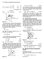
1.3.4 Set of Scales

Scales are used to make drawing of the objects to proportionate size desired. These are made of
wood, steel or plastic (Fig.I.3). BIS recommends eight set-scales in plastic/cardboard with

designations MI, M2 and so on as shown in Table 1.1 Set of scales

Fig. 1.3 Set of scales

Table 1.1 Set of Scales

Ml M2 M3 M4 M5 M6 M7 M8

Scale on one edge 1:1 1:2.5 1:10 1:50 1:200 1:300 1:400 1: 1000
Scale on other edge 1:2 1 :5 1:20 1:100 1:500 1.600 1:800 1:2000

Note: Do not use the scales as a straight edge for drawing straight lines.

These are used for drawing irregular curved lines, other than circles or arcs of circles.

Table 1.2

Scales for use on technical drawings (IS: 46-1988)
Category Recommended scales
Enlargement scales 50: I 20: I 10: 1

5: 1 2: 1

Full size I: 1

</div>
(15)<div class='page_container' data-page=15>

1.4 Textbook of Enginnering D r a w i n g

-1.3.5 French Curves

French curves are available in different shapes (Fig. 1.4). First a series of points are plotted along
the desired path and then the most suitable curve is made along the edge of the curve. A flexible
curve consists of a lead bar inside rubber which bends conveniently to draw a smooth curve
through any set of points.

(a) French curves (b) Flexible curve
Fig. 1.4

1.3.6 Tern plates

These are aids used for drawing small features such as circles, arcs, triangular, square and other
shapes and symbols used in various science and engineering fields (Fig.l.5).

Fig. 1.5 Template

1.3.7 Pencils

</div>
(16)<div class='page_container' data-page=16>

_ _ _ _ _ _ _ _ _ _ _ _ _ _ _ _ _ _ Drawing Instruments and Accessories 1.5

the numeral before the letter H increases. The lead becomes softer, as the value of the numeral
before B increases (Fig.l.6).

Hard

Soft

Fig. 1.6 Pencil Leads

The selection of the grade depends on the line quality desired for the drawing. Pencils of grades
H or 2H may be used for finishing a pencil drawing as these give a sharp black line. Softer grade
pencils are used for sketching work. HB grade is recommended for lettering and dimensioning.

Nowadays mechanical pencils are widely used in place of wooden pencils. When these are
used, much of the sharpening time can be saved. The number 0.5,0.70 of the pen indicates the
thickness of the line obtained with the lead and the size of the lead diameter.

Micro-tip pencils with 0.5 mm thick leads with the following grades are recommended.

Fig. 1.7 Mechanical Pencil

HB Soft grade for Border lines, lettering and free sketching

H Medium grade for Visible outlines, visible edges and boundary lines

2H Hard grade for construction lines, Dimension lines, Leader lines, Extension lines, Centre lines,

</div>
(17)<div class='page_container' data-page=17>

CHAPTER

2 Lettering and Dimensioning Practices

(As per BIS : SP : 46 : 2003)

2.1

Introduction

Engineering drawings are prepared on standard size drawing sheets. The correct shape and size
of the object can be visualised from the understanding of not only its views but also from the
various types of lines used, dimensions, notes, scale etc. For uniformity, the drawings must be
drawn as per certain standard practice. This chapter deals with the drawing practices as
recommended by Bureau of Indian Standards (BIS) SP: 46:2003. These are adapted from what is
followed by International Standards Organisation (ISO).

2.2

Drawing Sheet

The standard drawing sheet sizes are arrived at on the basic Principal of

x: y = 1 : -..12 and xy = 1 where x and yare the sides of the sheet. For example AO, having a surface

area of 1 Sq.m; x

=

841 rom and y

=

1189 mm. The successive sizes are obtained by either by

halving along the length or.doubling the width, the area being in the ratio 1 : 2. Designation of sizes
is given in Fig.2.l and their sizes are given in Table 2.1. For class work use of A2 size drawing
sheet is preferred.

Table 2.1

Designation Dimension, mm 
Trimmed size

AO 841 x 1189
A1 594 x 841
A2 420 x 594

A3 297 x 420
A4 210 x 297

</div>
(18)<div class='page_container' data-page=18>

2.2 Textbook of Enginnering D r a w i n g

-2.2.1 Title Block

The title block should lie within the drawing space at the bottom right hand comer of the sheet.
The title block can have a maximum length of 170 mm providing the following information.

1. Title of the drawing.

2. Drawing number.

3. Scale.

4. Symbol denoting the method of projection.

5. Name of the firm, and

6. Initials of staff who have designed, checked and approved.

The title block used on shop floor and one suggested for students class work are shown in
Fig.2.2.

170

..

NAME DATE MATERIAL TOLERANCE FINISH

DRN

CHD

~PP[
I/')

LEGAL

PROJECTION TITLE

OWNER

SCALE IDENTIFICATION NUMBER

Fig.2.2(a)

v

150

~ NAME OF

TITLE

STUDENT

=

CLASS: DRGNO: SCALE

-

=

ROLLNO: GRADE:

8 e

-'<

=

DATE:

-

VALUED BY

50

</div>
(19)<div class='page_container' data-page=19>

_ _ _ _ _ _ _ _ _ _ _ _ _ _ _ _ _ _ Lettering and Dimensioning Practices 2.3

2.2.2 Drawing Sheet Layout (Is 10711 : 2001)

The layout of a drawing sheet used on the shop floor is shown in Fig.2.3a, The layout suggested to
students is shown in Fig.2.3b.

Minimum Width

PD- FOR /11/ AND AI.

10_ FOR A2. A3 AND M)

_z I 4

~ II

~

•

Drawing Space

•

Edge

r

e 170 Title Bloc

--=---..

Arid'Reference

3 4 5

Fig. 2.2 (a) General features of a drawing sheet

s!

Filing Margin

...

2ID Drawing Space

Edge 170

~

Title Bloc k

v

a

..

5
Fig. 2.3 (b) Layout of sheet for class work

2.2.3 Folding of Drawing Sheets

IS : 11664 - 1999 specifies the method of folding drawing sheets. Two methods of folding of
drawing sheets, one suitable for filing or binding and the other method for keeping in filing cabinets
are specified by BIS. In both the methods offolding, the Title Block is always visible.

</div>
(20)<div class='page_container' data-page=20>

2.4 Textbook ofEnginnering D r a w i n g
-Sheet
Designation
A2
420x 594
Folding Diagram
190
;;;
~
....
'"
N
0
N

...

Lengthwise

Folding

Fig.2.4(a) Folding of drawing sheet for filing or binding

S94
174 (210) 210

I j

13FOlO I c;;

, I ~

r----r

,

420xS94

~I

...

a>

'"

..

""'

'"

N,

,

~Ir;-!!!!:U

BLOCK

Fig. 2.4(b) Folding of drawing sheet for storing in filing cabinet

2.2.4 Lines (IS 10714 (part 20): 2001 and SP 46: 2003)

Just as in English textbook the correct words are used for making correct sentences; in Engineering
Graphics, the details of various objects are drawn by different types of lines. Each line has a
defmite meaning and sense toconvey.

IS 10714 (Pint 20): 2001 (General principles of presentation on technical drawings) and SP 46:2003
specify the following types oflines and their applications:

• Visible Outlines, Visible .Edges : Type 01.2 (Continuous wide lines) The lines drawn
to represent the visible outlines/ visible edges / surface boundary lines of objects should be
outstanding in appearance.

• Dimension Lines: Type 01.1 (Continuous narrow Lines) Dimension Lines are drawn
to mark dimension.

</div>
(21)<div class='page_container' data-page=21>

_ _ _ _ _ _ _ _ _ _ _ _ _ _ _ _ _ _ Lettering and Dimensioning Practices 2.5

• Construction Lines: Type 01.1 (Continuous narrow Lines)

Construction Lines are drawn for constructing drawings and should not be erased after
completion of the drawing.

• Hatching / Section Lines: Type 01.1 (Continuous Narrow Lines)

Hatching Lines are drawn for the sectioned portion of an object. These are drawn inclined
at an angle of 45° to the axis or to the main outline of the section.

• Guide Lines: Type 01.1 (Continuous Narrow Lines)

Guide Lines are drawn for lettering and should not be erased after lettering.
• Break Lines: Type 01.1 (Continuous Narrow Freehand Lines)

Wavy continuous narrow line drawn freehand is used to represent bre~ of an object.
• Break Lines : Type 01.1 (Continuous Narrow Lines With Zigzags)

Straight continuous ~arrow line with zigzags is used to represent break of an object.
• Dashed Narrow Lines: Type 02.1 (Dashed Narrow Lines)

Hidden edges / Hidden outlines of objects are shown by dashed lines of short dashes of
equal lengths of about 3 mm, spaced at equal distances of about 1 mm. the points of intersection
of these lines with the outlines / another hidden line should be clearly shown.

• Center Lines: Type 04.1 (Long-Dashed Dotted Narrow Lines)

Center Lines are draWn at the center of the drawings symmetrical about an axis or both the
axes. These are extended by a short distance beyond the outline of the drawing.

• " Cutting Plane Lines: Type 04.1 and Type 04.2

Cutting Plane Line is drawn to show the location of a cutting plane. It is long-dashed dotted
narrow line, made wide at the ends, bends and change of direction. The direction of viewing
is shown by means of arrows resting on the cutting plane line.

• Border Lines

Border Lines are continuous wide lines of minimum thickness 0.7 mm

</div>
(22)<div class='page_container' data-page=22>

2.6 Textbook of Enginnering D r a w i n g

-..c

Fig. 2.6

Understanding the various types oflines used in drawing (i.e.,) their thickness, style of construction
and appearance as per BIS and following them meticulously may be considered as the foundation
of good drawing skills. Table 2.2 shows various types oflines with the recommended applications.

Table 2.2 Types of Lines and their applications (IS 10714 (Part 20): 2001) and BIS: SP46 : 2003.

No. Line description

and Representation
Ol.l Continuous narrow line

01.1 Continuous narrow freehand
line

C ~

01.1 Continuous narrow line with
zigzags

01.2 Continuous wide line

02.1 Dashed narrow line

- - - - -

-04.1 Long-dashed dotted narrow

- - . - _ ' _ -

line

04.2 Long-dashed dotted wide line

_ . '

-Line widths (IS 10714 : 2001)
Line width means line thickness.

Applications
Dimension lines, Extension lines

Leader lines, Reference lines
Short centre lines

Projection lines
Hatching

Construction lines, Guide lines
Outlines of revolved sections
Imaginary lines of intersection

Preferably manually represented tenrunation of partIal or
interrupted views, cuts and sections, if the limit is not a line of

symmetry or a center line·.

Preferably mechanically represented termination of partial or
interrupted vIews. cuts and sections, if the hmit is not a line of
symmetry or a center linea

Visible edges, visible outlines

Main representations in diagrams, ma~s. flow charts
Hidden edges

Hidden outlines

Center lines / Axes. Lines of symmetry

Cuttmg planes (Line 04.2 at ends and changes of direction)
Cutting planes at the ends and changes of direction outlines of
visible parts situated m front of cutting plane

Choose line widths according to the size of the drawing from the following range: 0.13,0.18,
0.25, 0.35, 0.5, 0.7 and 1 mm.

</div>
(23)<div class='page_container' data-page=23>

_ _ _ _ _ _ _ _ _ _ _ _ _ _ _ _ _ _ Lettering and Dimensioning Practices 2.7

Precedence of Lines

1. When a Visible Line coincide with a Hidden Line or Center Line, draw the Visible Line.
Also, extend the Center Line beyond the outlines of the view.

2. When a Hidden Line coincides with a Center Line, draw the Hidden Line.

3. When a Visible Line coincides with a Cutting Plane, draw the Visible Line.

4. When a Center line coincides with a Cutting Plane, draw the Center Line and show the
Cutting Plane line outside the outlines of the view at the ends of the Center Line by thick
dashes.

2.3 LETTERING [IS 9609 (PART 0) : 2001 AND SP 46 : 2003]

Lettering is defined as writing of titles, sub-titles, dimensions, etc., on a drawing.
2.3.1 Importance of Lettering

To undertake production work of an engineering components as per the drawing, the size and
other details are indicated on the drawing. This is done in the fonn of notes and dimensions.
Main Features of Lettering are legibility, unifonnity and rapidity of execution. Use of drawing 
instruments for lettering consumes more time. Lettering should be done freehand with speed.
Practice accompanied by continuous efforts would improve the lettering skill and style. Poor lettering
mars the appearance of an otherwise good drawing.

BIS and ISO Conventions

IS 9609 (Part 0) : 2001 and SP 46 : 2003 (Lettering for technical drawings) specifY lettering in
technical product documentation. This BIS standard is based on ISO 3098-0: 1997.

2.3.2 Single Stroke Letters

The word single-stroke should not be taken to mean that the lettering should be made in one stroke
without lifting the pencil. It means that the thickness of the letter should be unifonn as if it is
obtained in one stroke of the pencil.

2.3.3 Types of Single Stroke Letters

1. Lettering Type A: (i) Vertical and (ii) Sloped (~t 750 to the horizontal)

2. Lettering Type B : (i) Vertical and (ii) Sloped (at 750

to the horizontal)
Type B Preferred

In Type A, height of the capital letter is divided into 14 equal parts, while in Type B, height of the

capital letter is divided into 10 equal parts. Type B is preferred for easy and fast execution, because
of the division of height into 10 equal parts.

Vertical Letters Preferred

</div>
(24)<div class='page_container' data-page=24>

2.8 Textbook of Enginnering D r a w i n g

-Note: Lettering in drawing should be in CAPITALS (i.e., Upper-case letters).

Lower-case (small) letters are used for abbreviations like mm, cm, etc.

2.3.4 Size of Letters

• Size of Letters is measured by the height h of the CAPITAL letters as well as numerals.

• Standard heights for CAPITAL letters and numerals recommended by BIS are given below:

1.8, 2.5, 3.5, 5, 6, 10, 14 and 20 mm

Note: Size of the letters may be selected based upon the size of drawing.

Guide Lines

In order to obtain correct and uniform height ofletters and numerals, guide lines are drawn, using

2H pencil with light pressure. HB grade conical end pencil is used for lettering.
2.3.5 Procedure for Lettering

1. Thin horizontal guide lines are drawn first at a distance 'h' apart.

2. Lettering Technique: Horizontal lines of the letters are drawn from left to right. Vertical,

inclined and curved lines are drawn from top to bottom.

3. After lettering has been completed, the guidelines are not erased.

2.3.6 Dimensioning of Type B Letters (Figs 2.5 and 2.6)

BIS denotes the characteristics of lettering as :

h (height of capita) letters),

ci (height of lower-case letters),

c2 (tail of lower-case letters),

c3 (stem of lower-case letters),

a (spacing between characters),

bl & b2 (spacing between baselines),
e (spacing between words) and

d (line thickness),

Table 2.3 Lettering Proportions

Recommended Size (height h) of Letters I Numerals 
Main Title 5 mm, 7 mm, 10 mm

Sub-Titles 3.5 mm, 5 mm

</div>
(25)<div class='page_container' data-page=25>

_ _ _ _ _ _ _ _ _ _ _ _ _ _ _ _ _ _ _ Lettering and Dimensioning Practices 2.9

2.3.7 Lettering practice

Practice oflettering capital and lower case letters and numerals of type B are shown in Figs.2.7
and 2.8.

0 Base line Base line

£ .D

Base line
Base line

Fig. 2.7 Lettering

Fig. 2.8 Vertical Lettering

The following are some of the guide lines for lettering (Fig 2.9 & 2.10)

1. Drawing numbers, title block and letters denoting cutting planes, sections are written in
10 mrn size.

2. Drawing title is written in 7 mm size.

3. Hatching, sub-titles, materials, dimensions, notes, etc., are written in 3.5 mm size.
4. Space between lines = ~ h.

</div>
(26)<div class='page_container' data-page=26>

2.10 Textbook of Enginnering D r a w i n g - - - -_ _ _ _ _ _

Fig. 2.9 Inclined Lettering

6. Space between letters should be approximately equal to 115 h. Poor spacing will affect the
visual effect.

7. The spacing between two characters may be reduced by half if th is gives a better visual
effect, as for example LA, TV; over lapped in case of say LT, TA etc, and the space is
increased for letters with adjoining stems.

CAPITAL Letters

• Ratio of height to width for most of the CAPITAL letters is approximately = 10:6
• However, for M and W, the ratio = 10:8 for I the ratio = 10:2

Lower-case Letters

• Height of lower-case letters with stem I tail (b, d, f, g, h, j, k, I, p, q, t, y) = C

z = c3 = h

• Ratio of height to width for lower-case letters with stem or tail = 10:5

</div>
(27)<div class='page_container' data-page=27>

_ _ _ _ _ _ _ _ _ _ _ _ _ _ _ Lettering and Dimensioning Practices 2.11

Numerals

• For numerals 0 to 9, the ratio of height to width = 10 : 5. For I, ratio = 10 : 2
Spacing

• Spacing between characters

=

(2/10)b 
• Spacing between words = e

=

(6/10)b

SMALL

USED

SPACING

SPACES

SHOULD

BE

LETTER

FOR

GOOD

Correct

POOR

LETTER

SPACING

RES'U L T S

FRO

M SPA C E S

BEING

TOO BIG

In correct
Ca)

J. J.

NIGHT

NUMBERS

VITAL

t

Letters with adjoining Item.

require more Ipacing

ALTAR

tt

Lett.r combin.tlonl with over I.pping

len.,.

(b)

</div>
(28)<div class='page_container' data-page=28>

2.12 Textbook of Enginnering D r a w i n g

-Fig. 2.11 Vertical capital & Lowercase letters and numerals of type B

EXAMPLE IN LETTERING PRACTICE

Write freehand the following, using single stroke vertical CAPITAL letters of 5 mm (h) size

.J-

ENGINEERING GRAPHICS IS THE LANGUAGE

f

:!

OF ENGINEERS

Fig. 2.12

2.4 Dimensioning

</div>
(29)<div class='page_container' data-page=29>

_ _ _ _ _ _ _ _ _ _ _ _ _ _ _ _ _ _ Lettering and Dimensioning Practices 2.13

Rounds and
Fillets R3

General Note ~

I\J 54

r

Extension line

DimensIon

...,

ReferenceI-.Dl-im-e-nS-io-n-~'1I---;;'-=--D-i-m-e-n-1s~ion""'lIne

,c- Local Note
C' BORE

DIA 28. DEEP 25

DIA 20 D~E:.'::E:.':.P~37---r-"V'--_ _ L

R15

Centre Line used as
an ExtensIon Lane

Dimensions in Millimetres ~
units of Measurements

-e-.-$

Frojection Symbol

~

Fig.2.13 Elements of Dimensioning

2.4.1 Principles of Dimensioning

Some of the basic principles of dimensioning are given below.

I. All dimensional information necessary to describe a component clearly and completely shall
be written directly on a drawing.

2. Each feature shall be dimensioned once only on a drawing, i.e., dimension marked in one
view need not be repeated in another view.

3. Dimension should be placed on the view where the shape is best seen (Fig.2.14)

4. As far as possible, dimensions should be expressed in one unit only preferably in millimeters,
without showing the unit symbol (mm).

5. As far as possible dimensions should be placed outside the view (Fig.2.15).

</div>
(30)<div class='page_container' data-page=30>

2.14 Textbook of Enginnering D r a w i n g

-13

CORRECT INCORRECT

Fig. 2.14 Placing the Dimensions where the Shape is Best Shown

~r$-

-

50

CORRECT INCORRECT

Fig. 2.15 Placing Dimensions Outside the View

Correct

10 26
Incorrect

Fig. 2.16 Marking the dimensions from the visible outlines

</div>
(31)<div class='page_container' data-page=31>

_ _ _ _ _ _ _ _ _ _ _ _ _ _ _ _ _ _ Lettering and Dimensioning Practices 2.15

22
52
Correct

52
Incorrect

Fig. 2.17 Marking of Extension Lines

Correct Incorrect

Fig. 2.18 Crossing of Centre Lines

2.4.2 Execution of Dimensions

1. Prejection and dimension lines should be drawn as thin continuous lines. projection lines
should extend slightly beyond the respective dimension line. Projection lines should be drawn
perpendicular to the feature being dimensioned. If the space for dimensioning is insufficient,
the arrow heads may be reversed and the adjacent arrow heads may be replaced by a dot
(Fig.2.19). However, they may be drawn obliquely, but parallel to each other in special cases,
such as on tapered feature (Fig.2.20).

~

.1

°1.

1 30 .1
20

4=4=

</div>
(32)<div class='page_container' data-page=32>

2.16 Textbook of Enginnering D r a w i n g

-Fig. 2.20 Dimensioning a Tapered Feature

2. A leader line is a line referring to a feature (object, outline, dimension). Leader lines should
be inclined to the horizontal at an angle greater than 30°. Leader line should tenninate,
(a) with a dot, if they end within the outline ofan object (Fig.2.21a).

(b) with an arrow head, if they end on outside of the object (Fig.2.21b).

(a) (b) (c)

Fig. 2.21 Termination of leader lines

Dimension Termination and Origin Indication

Dimension lines should show distinct tennination in the fonn of arrow heads or oblique strokes or
where applicable an origin indication (Fig.2.22). The arrow head included angle is 15°. The origin
indication is drawn as a small open circle of approximately 3 mm in diameter. The proportion lenght
to depth 3 : 1 of arrow head is shown in Fig.2.23.

-I

---~o

Fig. 2.22 Termination of Dimension Line

~..l. ... _ ,.& _ _ A _ _ ... "' __ ...1

</div>
(33)<div class='page_container' data-page=33>

_ _ _ _ _ _ _ _ _ _ _ _ _ _ _ _ _ _ Lettering and Dimensioning Practices 2.17

When a radius is dimensioned only one arrow head, with its point on the arc end of the dimension
line should be used (Fig.2.24). The arrow head termination may be either on the inside or outside
of the feature outline, depending on the size of the feature.

Fig. 2.24 Dimensioning of Radii

2.4.3 Methods of Indicating Dimensions

The dimensions are indicated on the drawings according to one of the following two methods.

Method - 1 (Aligned method)

Dimensions should be placed parallel to and above their dimension lines and preferably at the
middle, and clear of the line. (Fig.2.25).

Fig. 2.25 Aligned Method

Dimensions may be written so that they can be read from the bottom or from the right side of
the drawing. Dinensions on oblique dimension lines should be oriented as shown in Fig.2.26a and
except where unavoidable, they shall not be placed in the 30° zone. Angular dimensions are oriented
as shown in Fig.2.26b

Method - 2 (uni-directional method)

Dimensions should be indicated so that they can be read from the bottom of the drawing only.
Non-horizontal dimension lines are interrupted, preferably in the middle for insertion of the dimension
(Fig.2.27a).

Angular dimensions may be oriented as in Fig.2.27b

</div>
(34)<div class='page_container' data-page=34>

2.18 Textbook of Enginnering D r a w i n g

-(a) (b)

Fig.2.26 Angular Dimensioning

f20 .30 +50

26 10

(a) (b)

Fig.2.27 Uni-directional Method

2.4.4 Identification of Sbapes

The following indications are used with dimensions to show applicable shape identification and to
improve drawing interpretation. The diameter and square symbols may be omitted where the shape
is clearly indicated. The applicable indication (symbol) shall precede the value for dimension
(Fig. 2.28 to 2.32).

Fig. 2.28

</div>
(35)<div class='page_container' data-page=35>

_ _ _ _ _ _ _ _ _ _ _ _ _ _ _ _ _ Lettering and Dimensioning Practices 2.19

2.5

Arrangement of Dimensions

a
..:#

o

Fig. 2.30

Fig. 2.31

Fig. 2.32

The arrangement of dimensions on a drawing must indicate clearly the purpose of the design of the
object. They are arranged in three ways.

1. Chain dimensioning
2. Parallel dimensioning
3. Combined dimensioning.

1. Chain dimensioning

Chain of single dimensioning should be used only where the possible accumulation of tolerances

does not endanger the fundamental requirement of the component (Fig.2.33)

2. Parallel dimensioning

In parallel dimensioning, a number of dimension lines parallel to one another and spaced out,

are used. This method is used where a number of dimensions have a common datum feature

</div>
(36)<div class='page_container' data-page=36>

2.20 Textbook of Enginnering D r a w i n g

-('I)
~

('I)
(Q

-16{) 30 85

l!i

Fig. 2.33 Chain Dimensioning

,

64-179

272

Fig. 2.34 Parallel Dimensioning

-r - - - I

-- -

-

--

</div>
(37)<div class='page_container' data-page=37>

_ _ _ _ _ _ _ _ _ _ _ _ _ _ _ _ _ _ Lettering and Dimensioning Practices 2.21

Violation of some of the principles of drawing are indicated in Fig.2.36a. The corrected

version of the same as per BIS SP 46-2003 is given is Fig.2.36b. The violations from 1 to 16

indicated in the figure are explained below.

I

~1~

, , 
,

I L~

: . I

I

! . : I~t

,ko

J

FRONTVlEW

TOPVl£W'

(a) (b)

Fig. 2.36
1. Dimension should follow the shape symbol.

2. and 3. As far as possible, features should not be used as extension lines for dimensioning.
4. Extension line should touch the feature.

5. Extension line should project beyond the dimension line.
6. Writing the dimension is not as per aligned method.
7. Hidden lines should meet without a gap.

S. Centre line representation is wrong. Dots should be replaced by small dashes.

9. Horizontal dimension line should not be broken to insert the value of dimension in both aligned
and uni-direction methods.

10. Dimension should be placed above the dimension line.
11. Radius symbol should precede the dimension.

12. Centre line should cross with long dashes not short dashes.

13. Dimension should be written by symbol followed by its values and not abbreviation.
14. Note with dimensions should be written in capitals.

</div>
(38)<div class='page_container' data-page=38>

2.22 Textbook of Enginnering D r a w i n g - - - -_ _

~100

H - 1 2 0

(a) Incorrect

1 + - - -40 - - - - + I

(a) Incorrect

40$

Fig. 2.37

Fig. 2.38

Fig. 2.39
8

120
100

(b) Correct

3 HOLES

DIA 10

~..,
7f~---+~~..,

(b) Correct

</div>
(39)<div class='page_container' data-page=39>

_ _ _ _ _ _ _ _ _ _ _ _ _ _ _ _ _ _ _ Lettering and Dimensioning Practices 2.23

-:.-o

'"

...

(b) Correct

Fig. 2.40

15 20

Fig. 2.41

Fig. 2.42

1 + - - -.... -:20

</div>
(40)<div class='page_container' data-page=40>

2.24 Textbook of Enginnering D r a w i n g - - - -_ _ _ _ _ _ _

1l1li 15

~ _ _ 40

,I

Fig. 2.44

I I

-+I 20 ~ 14- ~

I I

_.J _ _ _ .1_

Fig. 2.45

---

....

~20 20 15

Fig. 2.46

Drill ~ 10, C Bore <p 20

</div>
(41)<div class='page_container' data-page=41>

_ _ _ _ _ _ _ _ _ _ _ _ _ _ _ _ Lettering and Dimensioning Practices, 2.25

4CMd

EXERCISE

r

SCM

i

LI--_ _

----I

T

SCM

Fig. 2.48

+

~ 25 - +

Fig. 2.49

Fig. 2.50

t

5CM

t

Write freehand the following, using single stroke vertical (CAPITAL and lower-case) letters:

1. Alphabets (Upper-case & Lower-case) and Numerals 0 to 9 (h

=

5 and 7 nun)

2. PRACTICE MAKES A PERSON PERFECT (h

=

3.5 and 5)

3. BE A LEADER NOT A FOLLOWER (h = 5)

</div>
(42)<div class='page_container' data-page=42>

CHAPTER

3 Scales

3.1 Introduction

It is not possible always to make drawings of an object to its actual size. If the actual linear

dimensions of an object are shown in its drawing, the scale used is said to be a full size scale.

Wherever possible, it is desirable to make drawings to full size.
3.2

Reducing and Enlarging

Scales

Objects which are very big in size can not be represented in drawing to full size. In such cases the
object is represented in reduced size by making use of reducing scales. Reducing scales are used
to represent objects such as large machine parts, buildings, town plans etc. A reducing scale, say
1: 10 means that 10 units length on the object is represented by 1 unit length on the drawing.

Similarly, for drawing small objects such as watch parts, instrument components etc., use offull
scale may not be useful to represent the object clearly. In those cases enlarging scales are used.

An enlarging scale, say 10: 1 means one unit length on the object is represented by 10 units on the
drawing.

The designation of a scale consists of the word. SCALE, followed by the indication of its ratio
as follows. (Standard scales are shown in Fig. 3.1)

Scale 1: 1 for full size scale

Scale 1: x for reducing scales (x

=

10,20 ... etc.,)
Scale x: 1 for enlarging scales.

Note: For all drawings the scale has to be mentioned without fail.

r

111111111111111111111111111111111111111111111111111

1:1 0 10 20 30 40 50

r

IIIIIIIIIIIIIIIIIIIIIIIIIIIIIIIIIIIIIIITIIIIIIIII

1:5 0 100 200

r

111111111111111111111111111111111111111111111111111

1.2 0 20 40 60 80 100

r

1IIIIIIIIIIIIIIIIIIIIIIIIIIIIIIIIIImllllllllllili

1.100 200 400

</div>
(43)<div class='page_container' data-page=43>

3.2 Textbook of Enginnering D r a w i n g

-3.3 Representative Fraction

The ratio of the dimension of the object shown on the drawing to its actual size is called the
Representative Fraction (RF).

RF = Drawing size of an object (. m same umts . )
Its actual size

F or example, if an actual length of3 metres of an object is represented by a line of 15mm length
on the drawing

RF = 15mm = lSmm =_1_ orl:200
3m (3 x 1000)mm 200

If the desired scale is not available in the set of scales it may be constructed and then used.

Metric Measurements

10 millimetres (mm) = 1 centimetre( cm)
10 centimetres (cm) = 1 decimetre(dm)
10 decimetre (dm) = 1 metre(m)
10 metres (m) = 1 decametre (dam)
10 decametre (dam) = 1 hectometre (bm)
10 hectometres (bm) = 1 kilometre (km)
1 hectare = 10,000 m2

3.4 Types of Scales

The types of scales normally used are:
1. Plain scales.

2. Diagonal Scales.
3. Vernier Scales.

3.4.1 Plain Scales

A plain scale is simply a line which is divided into a suitable number of equal parts, the fIrst of
which is further sub-divided into small parts. It is used to represent either two units or a unit and its
fraction such as km and bm, m and dm, cm and mm etc.

Problem 1 : On a survey map the distance between two places 1 km apart is 5 cm. Construct

the scale to read 4.6 km.

Solution: (Fig 3.2)

Scm 1

RF= =

</div>
(44)<div class='page_container' data-page=44>

---Scru~ 3.3

Ifx is the drawing size required x = 5(1000)(100) x 20000

Therefore, x = 25 cm

Note: If 4.6 km itself were to be taken x

=

23 cm. To get 1 km divisions this length has to be

divided into 4.6 parts which is difficult. Therefore, the nearest round figure 5 km is considered.

When this length is divided into 5 equal parts each part will be 1 km.

1. Draw a line of length 25 cm.

2. Divide this into 5 equal parts. Now each part is 1 km.

3. Divide the first part into 10 equal divisions. Each division is 0.1 km.

4. Mark on the scale the required distance 4.6 km.

46km

I I I I I I I I I I I I I
I

I I I I I

10 5 0 1 2 3 4

HECfOMETRE LENGTH OFTHE SCALE KILOMETRE

SCALE .1.20000

Fig. 3.2 Plain Scale

Problem 2 : Construct a scale of 1:50 to read metres and decimetres and long enough to

measure 6 m. Mark on it a distance of 5.5 m.

Construction (Fig. 3.3)

1. Obtairrthe length of the scale as: RF x 6m

=

_1 x 6 x 100

=

12 cm

2. Draw a rectangle strip oflength 12 cm and width 0.5 cm.

3. Divide the length into 6 equal parts, by geometrical method each part representing 1m.
4. Mark O(zero) after the first division and continue 1,2,3 etc., to the right of the scale.
5. Divide the first division into 10 equal parts (secondary divisions), each representing 1 cm.
6. Mark the above division points from right to left.

7. Write the units at the bottom of the scale in their respective positions.

8. Indicate RF at the bottom of the figure.

</div>
(45)<div class='page_container' data-page=45>

3.4 Textbook of Enginnering D r a w i n g

--'I

5.5m

;(1

if

t

j

I I I I I

10 5 o 2

3 4 5

DECIMETRE RF=l/50 METRES

Fig. 3.3

Problem 3 : The distance between two towns is 250 km and is represented by a line of

length 50mm on a map. Construct a scale to read 600 km and indicate a distance of 530 km

on it.

Solution: (F ig 3.4)

50 1

50mm

1. Determine the RF value as

-250km 250x 1000x 1000

=

5 X 106

2. Obtain the length of the scale as: 1 x 600km

=

120mm .

5xl06

3. Draw a rectangular strip oflength 120 mm and width 5 mm.

4. Divide the length into 6 eq1}AI parts, each part representing 10 km.

5. Repeat the steps 4 to 8 of construction in Fig 3.2. suitably.

6. Mark the distance 530 km as shown.

/

II

~

if

j.

I

I I II I

100 50 0

100

530km

I I

300

Fig. 3.4

</div>
(46)<div class='page_container' data-page=46>

- - - S c a l e s 3.5

Problem 4: Construct a plain scale of convenient length to measure a distance of 1 cm and

mark on it a distance of 0.94 em. 
Solution: (Fig 3.5)

This is a problem of enlarged scale.

1. Take the length of the scale as 10 cm

2. RF

=

1011, scale is 10:1

3. The construction is shown in Fig 3.5

094cm

1111

1 0 1 Z 3 4 5 6 7 89

LENG1H OFTHE SCAlE 100mm
SCAlE: 1:1

Fig. 3.5

3.4.2 Diagonal Scales .

Plain scales are used to read lengths in two units such as metres and decimetres, centimetres and
millimetres etc., or to read to the accuracy correct to first decimal.

Diagonal scales are used to represent either three units of measurements such as metres,

decimetres, centimetres or to read to the accuracy correct to two decimals.

Principle of Diagonal Scale (Fig 3.6)

1. Draw a line AB and errect a perperrdicular at B.

2. Mark 10 equi-distant points (1,2,3, etc) of any suitable length along this perpendicular and
mark C.

3. Complete the rectangle ABCD
4. Draw the diagonal BD.

5. Draw horizontals through the division points to meet BD at l' , 2' , 3' etc.
Considering the similar triangles say BCD and B44'

B4' B4 4 I 4 ,

- = _ . =-xBCx-=-· 44 =O.4CD

</div>
(47)<div class='page_container' data-page=47>

3.6

Textbook of Enginnering Drawing

0 C

9
9'

7' 7

6
6'
5
5'
4
4'
3
3'
2
2'
1

A B

Fig. 3.6 Principle of Diagonal Scale

Thus, the lines 1-1',2 - 2', 3 - 3' etc., measure O.lCD, 0.2CD, 0.3CD etc. respectively. Thus,
CD is divided into 1110 the divisions by the diagonal BD, i.e., each horizontal line is a multiple of 11
10 CD.

This principle is used in the construction of diagonal scales.

Note: B C must be divided into the same number of parts as there are units of the third dimension

in one unit of the secondary division.

Problem 5 : on a plan, a line of 22 em long represents a distance of 440 metres. Draw a 
diagonal scale for the plan to read upto a single metre. Measure and mark a distance of 187 
m on the scale.

Solution: (Fig 3.7)

187m
DEC I5ETRE

\ \

1\ \

\

\ \

t

\ \

\

\ \

\ \ \ \

\ \

\

o \ \

I

40 211 0 40 80 1211 160
LENGTH OF SCALE 100mm MeIJ&

SOUE.1:2000

</div>
(48)<div class='page_container' data-page=48>

- - - S C a l e s 3.7

22 1

1. RF

=

440xl00

=

2000

2. As 187 m are required consider 200 m.

Therefore drawing size

=

R F x actual size

=

2000 x 200 x 100

=

10 em

When a length of 1 0 cm representing 200 m is divided into 5 equal parts, each part represents
40 m as marked in the figure.

3. The first part is sub-divided into 4 divisions so that each division is 10 cm

4. On the diagonal portion 10 divisions are taken to get 1 m.

5. Mark on it 187 m as shown.

Problem 6 : An area of 144 sq cm on a map represents an area of 36 sq /an on the field. Find

the RF of the scale of the map and draw a diagonal scale to show Km, hectometres and

decametres and to measure upto 10 /an. Indicate on the scale a distance 7 /an, 5 hectometres

and 6 decemetres.

Solution: (Fig. 3.8)

1. 144 sq cm represents 36 sq km or 12 cm represent 6 km

12 1

=

6xl000xl00

=

50000
10xl000xl00

Drawing size x

=

R F x actual size

=

20 cm
50000

CA Mem:

1111

10 5 0

HECTOMETRE

7.56Icm

1 3 5 7

LENGTH Of THE SCALE KILOMETRE

Fig. 3.8

</div>
(49)<div class='page_container' data-page=49>

3.8 Textbook of Enginnering D r a w i n g
-2. Draw a length of 20 cm and divide it into 10 equal parts. Each part represents 1 km.
3. Divide the first part into 10 equal subdivisions. Each secondary division represents 1 hecometre
4. On the diagonal scale portion take 10 eqal divisions so that 1110 ofhectometre

=

1 decametre

is obtained.

5. Mark on it 7.56 km. as shown.

Problem 7 : Construct a diagonal scale 1/50, showing metres, decimetres and centimetres,

to measure upto 5 metres. Mark a length 4. 75 m on it.

Solution: (Fig 3.9)

1. Obatin the length of the scale as _1 x 5 x 100

=

10 cm
50

2. Draw a line A B, 10 cm long and divide it into 5 equal parts, each representing 1 m.

3-. -Divide the fIrst part into 10 equal parts, to represent decimetres.

4. Choosing any convenient length, draw 10 equi-distant parallel lines alJove AB and complete
the rectangle ABC D.

5. Erect perpendiculars to the line A B, through 0, 1,2,3 etc., to meet the line C D.

6. Join D to 9, the fIrst sub-division from A on the main scale AB, forming the fIrst diagonal.
7. Draw the remaining diagonals, parallel to the fIrst. Thus, each decimetre is divided into II

10th division by diagonals.
8. Mark the length 4.75m as shown.

.... w 
:i
~
w
o
0
10
8
6
4
2

A1()~

J;!fCIMETEB
Q
4.75m
c

1 2 3 4 5

FtF = 1:50 METRES

</div>
(50)<div class='page_container' data-page=50>

- - - S c a l e s 3.9

3.4.3 Vernier Scales

The vernier scale is a short auxiliary scale constructed along the plain or main scale, which can
read upto two decimal places.

The smallest division on the main scale and vernier scale are 1 msd or 1 vsd repectively.
Generally (n+ 1) or (n-l) divisions on the main scale is divided into n equal parts on the vernier
scale.

(n -1)

(1)

Thus, 1 vsd = -n-msd or 1-; msd

When 1 vsd < 1 it is called forward or direct vernier. The vernier divisions are numbered in the
same direction as those on the main scale.

When 1 vsd> 1 or (1 + lin), It is called backward or retrograde vernier. The vernier divisions
are numbered in the opposite direction compared to those on the main scale.

The least count (LC) is the smallest dimension correct to which a measurement can be made
with a vernier.

For forward vernier, L C = (1 msd - 1 vsd)
For backward viermier, LC = (1 vsd - 1 msd)

Problem 8 : Construct a forward reading vernier scale to read distance correct to decametre

on a map in which the actual distances are reduced in the ratio of 1 : 40,000. The scale

should be long enough to measure upto 6 km. Mark on the scale a length of 3.34 km and

0.59 km.

Solution: (Fig. 3.10)

6xl000x 100

1. RF = 1140000; length of drawing = 40000 = 15 em

2. 15 em is divided into 6 parts and each part is 1 km

3. This is further divided into 10 divitions and each division is equal to 0.1 km = 1 hectometre.
Ims d = 0.1 km = 1 hectometre

L.C expressed in terms of m s d = (111 0) m s d
L C is 1 decametre = 1 m s d - 1 v s d

1 v s d = 1 - 1110 = 9110 m s d = 0.09 km

4. 9 m sd are taken and divided into 10 divisions as shown. Thus 1 vsd = 9110 = 0.09 km
5. Mark on itbytaking6vsd=6x 0.9 = 0.54km, 28msd(27 + 1 on the LHS of 1) =2.8 kmand

Tota12.8 + 0.54 = 3.34 km.

</div>
(51)<div class='page_container' data-page=51>

3.10 Textbook of Enginnering D r a w i n g
-O.54+2.S=3.34lcm

O.SSkm

o

5 10

LENGTH OF THE SCALE 150 mm

SCAlE:1:40000

Fig. 3.10 Forward Reading Vernier Scale

Problem 9 : construct a vernier scale to read metres, decimetres and centimetres and long 
enough to measure upto 4m. The RF of the scale in 1120. Mark on it a distance of 2.28 m.

Solution: (Fig 3.11)

Backward or Retrograde Vernier scale

1. The smallest measurement in the scale is cm.

Therefore LC

=

O.Olm

2. Length of the scale

=

RF x Max. Distance to be measured

1 1

= -

x 4m

= -

x 400

=

20 em

20 20

LeastCO\.llt= O.01m

Rf" 1120

</div>
(52)<div class='page_container' data-page=52>

- - - S c a l e s

3.11

3. Draw a line of20 em length. Complete the rectangle of20 em x 0.5 em and divide it into
4 equal parts each representing 1 metre. Sub divide all into 10 main scale divisions.

1 msd = Im/l0 = Idm.

4. Take 10+ 1 = 11 divisions on the main scale and divide it into 10 equal parts on the vernier
scale by geometrical construction.

Thus Ivsd= llmsd/lO= 1.1dm= llcm

5. Mark 0,55, 110 towards the left from 0 (zero) on the vernier scale as shown.
6. Name the units of the divisions as shown.

7. 2.28m = (8 x vsd) + 14msd)

= (8 x O.llm) + (14 x O.lm)

</div>
(53)<div class='page_container' data-page=53>

3.12 Textbook of Enginnering D r a w i n g

-EXERCISES

1. Construct a plain scale of 1 :50 to measure a distance of 7 meters. Mark a distance of
3.6 metres on it.

2. The length of a scale with a RF of2:3 is 20 cm. Construct this scale and mark a distance of
16.5 cm on it.

3. Construct a scale of 2 cm = 1 decimetre to read upto 1 metre and mark on it a length of
0.67 metre.

4. Construct a plain scale of RF = 1 :50,000 to show kilometres and hectometres and long
enough to measure upto 7 krn. Mark a distance of 5:3 kilometres on the scale.

5. On a map, the distance between two places 5 krn apart is 10 cm. Construct the scale to read
8 krn. What is the RF of the scale?

6. Construct a diagonal scale ofRF = 1150, to read metres, decimetres and centimetres. Mark
a distance of 4.35 krn on it.

7. Construct a diagonal scale of five times full size, to read accurately upto 0.2 mm and mark
a distance of 3 .65 cm on it.

8. Construct a diagonal scale to read upto 0.1 mm and mark on it a 'distance of 1.63 cm and
6.77 cm. Take the scale as 3: 1.

9. Draw a diagonal scale of 1 cm = 2.5krn and mark on the scale a length of26.7 krn.
10. Construct a diagonal scale to read 2krn when its RF=I:20,000. Mark on it a distance of

1:15 km.

11. Draw a venier scale of metres when Imm represents 25cm and mark on it a length of
24.4 cm and 23.1 mm. What is the RF?

12. The LC of a forward reading vernier scale is 1 cm. Its vernier scale division represents
9 cm. There are 40 msd on the scale. It is drawn to 1 :25 scale. Construct the scale and mark
on it a distance ofO.91m.

</div>
(54)<div class='page_container' data-page=54>

CHAPTER

4 Geometrical Constructions

4.1 Introduction

Engineering drawing consists of a number of geometrical constructions. A few methods are
illustrated here without mathematical proofs.

1. To divide a straight line into a given number of equal parts say 5.

construction (Fig.4.1)

"

2' 3' 4' B

I

c

Fig. 4.1 Dividing a line

1. Draw AC at any angle

e

to AB.

2. Construct the required number of equal parts of convenient length on AC like 1,2,3.
3. Join the last point 5 to B

4. Through 4, 3, 2, 1 draw lines parallel to 5B to intersect AB at 4',3',2' and 1'.
2. To divide a line in the ratio 1 : 3 : 4.

</div>
(55)<div class='page_container' data-page=55>

4.2 Textbook of Enginnering D r a w i n g

-As the line is to be divided in the ratio 1:3:4 it has to be divided into 8 equal divisions.
By following the previous example divide AC into 8 equal parts and obtain P and Q to divide
the lineAB in the ratio 1:3:4.

A~~---~---~

3. To bisect a given angle.
construction (Fig.4.3)

Fig. 4.2

Fig. 4.3
1. Draw a line AB and AC making the given angle.

c

..

2. With centre A and any convenient radius R draw an arc intersecting the sides at
D and E.

3. With centres D and E and radius larger than half the chord length DE, draw arcs
intersecting at F

4. JoinAF, <BAF

=

<PAC.

4. To inscribe a square in a given circle.
construction (Fig. 4.4)

1. With centre 0, draw a circle of diameter D.

2. Through the centre 0, drwaw two diameters, say AC and BD at right angle to each
other.

</div>
(56)<div class='page_container' data-page=56>

_ _ _ _ _ _ _ _ _ _ _ _ _ _ _ _ _ _ _ _ _ GeometricaIContructions 4.3

c

8
Fig. 4.4

5. To inscribe a regular polygon of any number of sides in a given circle.
construction (Fig. 4.5)

>f

/

Fig. 4.5

1. Draw the given circle with AD as diameter.
2. Divide the diameter AD into N equal parts say 6.

3. With AD as radius and A and D as centres, draw arcs intersecting each other at G

</div>
(57)<div class='page_container' data-page=57>

4.4 Textbook of Enginnering D r a w i n g
-5. loinA-B which is the length of the side of the required polygon.

6. Set the compass to the length AB and strating from B mark off on the circuference of
the circles, obtaining the points C, D, etc.

The figure obtained by joing the points A,B, C etc., is the required polygon.

6. To inscribe a hexagon in a given circle.

(a) Construction (Fig. 4.6) by using a set-square or mini-draughter

o

2 2

21

A 0

2~,

60' 60'

Fig. 4.6

1. With centre 0 and radius R draw the given crcle.
2. Draw any diameter AD to the circle.

3. Using 30° - 60° set-square and through the point A draw lines AI, A2 at an angle 60°
with AD, intesecting the circle at B and F respectively.

4. Using 30° - 60° and through the point D draw lines Dl, D2 at an angle 60° with DA,
intersecting the circle at C and E respectively.

By joining A,B,C,D,E,F, and A the required hexagon is obtained.
(b) Construction (Fig.4.7) By using campass

1. With centre 0 and radius R draw the given circle.
2. Draw any diameter AD to the circle.

3. With centres A and D and radius equal to the radius of the circle draw arcs intesecting
the circles at B, F, C and E respectively.

</div>
(58)<div class='page_container' data-page=58>

- - - -_ _ _ _ _ _ _ _ _ GeometricaIContructions 4.5

...---f...-o''---.

Fig. 4.7

7. To circumscribe a hexagon on a given circle of radius R
construction (Fig. 4.8)

\
\

/

\t-+---1--B

R/
I

I

+0

Fig. 4.8

c

I. With centre 0 and radius R draw the given circle.

/

o

2. Using 60° position of the mini draughter or 300-600set square, circumscribe the hexagon
as shown.

8. To construct a hexagon, given the length of the side.
(a) contruction (Fig. 4.9) Using set square

1. Draw a line AB equal to the side of the hexagon.

</div>
(59)<div class='page_container' data-page=59>

4.6 Textbook of Enginnering D r a w i n g

-1 2

\

A . ..---'---+---'----t'

A B

Fig. 4.9

3. Through 0, the point of intesection between the lines A2 at D and B2 at E.
4. loinD,E

5. ABC D E F is the required hexagon.
(b) By using compass (Fig.4.10)

x

a

Fig. 4.10
D

B

1. Draw a line AB equal to the of side of the hexagon.

c

2. With centres A and B and radius AB, draw arcs intersecting at 0, the centre of the
hexagon.

3. With centres 0 and B and radius OB (=AB) draw arcs intersecting at C.
4. Obtain points D, E and F in a sinilar manner.

9. To construct a regular polygon (say a pentagon) given the length of the side.
construction (Fig.4.11)

</div>
(60)<div class='page_container' data-page=60>

- - - ' - - - G e o m e t r i c a l Contructions 4.7

Fig. 4.11

3. Join B to second division

2. Irrespective of the number of sides of the polygon B is always joined to the second
division.

4. Draw the perpendicular bisectors of AB and B2 to intersect at O.
5. Draw a circle with 0 as centre and OB as radius.

6. WithAB as radius intersect the circle successively at D and E. Thenjoin CD. DE and EA.
10. To construct a regular polygon (say a hexagon) given the side AB - alternate

method.

construction (Fig.4.12)

E

A

Fig. 4.12

1. Steps 1 to 3 are same as above
2. Join B- 3, B-4, B-5 and produce them.

3. With 2 as centre and radius AB intersect the line B, 3 produced at D. Similarly get the
point E and F.

</div>
(61)<div class='page_container' data-page=61>

4.8 Textbook of Enginnering D r a w i n g
-11. To construct a pentagon, given the length of side.

(a) Construction (Fig.4.13a)

F

1. Draw a line AB equal to the given length of side.
2. Bisect AB at P.

3. Draw a line BQ equal to AB in length and perpendicular to AB.

4. With centre P and radius PQ, draw an arc intersecting AB produced at R. AR is equal to

the diagonal length of the pentagon.

S. With centres A and B and radii AR and AB respectively draw arcs intersecting at C.
6. With centres A and B and radius AR draw arcs intersecting at D.

7. With centres A and B and radii AB and AR respectively draw arcs intersecting at E.
ABCDE is the required pentagon.

2 R

A

Fig.4.13a

(b)By included angle method

1. Draw a line AB equal to the length of the given side.
2. Draw a line B 1 such that <AB 1 = 108° (included angle)

3. Mark Con Bl such that BC = AB

4. Repeat steps 2 and 3 and complete the pentagon ABCDE

Fig.4.13b

/

,I'

1 C

12. To construct a regular figure of given side length and of N sides on a straight line.
construction (Fig 4.14)

1. Draw the given straight line AB.

2. At B erect a perpendicular BC equal in length to AB.

3. Join AC and where it cuts the perpendicular bisector of AB, number the point 4.
4. Complete the square ABeD of which AC is the diagonal.

</div>
(62)<div class='page_container' data-page=62>

- _ _ _ _ _ _ _ _ _ _ _ _ _ _ _ _ _ _ _ _ Geometrical Contructions 4.9

Fig. 4.14

6. Where this arc cuts the vertical centre line number the point 6.

7. This is the centre of a circle inside which a hexagon of side AB can now be drawn.
8. Bisect the distance 4-6 on the vertical centre line.

9. Mark this bisection 5. This is the centre in which a regular pentagon of side AB can now
be drawn.

10. On the vertical centre line step off from point 6 a distance equal in length to the distance
5-6. This is the centre of a circle in which a regular heptagon of side AB can now be

drawn.

11. If further distances 5-6 are now stepped off along the vertical centre line and are numbered
consecutively, each will be the centre of a circle in which a regular polygon can be
inscribed with sice of length AB and with a number of sides denoted by the number
against the centre.

13. To inscribe a square in a triangle.
construction (Fig. 4.15)

1. Draw the given triangle ABC.

2. From C drop a perpendicular to cut the base AB at D.
3. From C draw CE parallel toAB and equal in length to CD.
4. Draw AE and where it cuts the line CB mark F.

5. From F draw FG parallel to AB.
6. From F draw F J parallel to CD.
7. From G draw GH parallel to CD.
8. Join H to 1.

</div>
(63)<div class='page_container' data-page=63>

4.10 Textbook of Enginnering D r a w i n g

-C E

/

'""

, /

/ '

'\ /~

\.. /

!

"-"-, 
\

""

I

"-A

,

H 0 J B

Fig. 4.15

14. To inscribe within a given square ABCD, another square, one angle of the required
square to touch a side of the given square at a given point

construction (Fig 4.16)

Fig. 4.16

1. Draw the given square ABeD.

2. Draw the diagonals and where they intersect mark the point O.

3. Mark the given point E on the line AB.

4. With centre 0 and radius OE, draw a circle.

S. Where the circle cuts the given square mark the points G, H, and F.

6. Join the points GHFE.

Then GHFE is the required square.

15. To draw an arc of given radius touching two straight lines at right 8rngles to each _
other.

construction (Fig 4.17)

Let r be the given radius and AB and AC the given straight lines. With A as centre and
radius equal to r draw arcs cutting AB at P and Q. With P and Q as centres draw arcs to

</div>
(64)<div class='page_container' data-page=64>

- - - - -_ _ _ _ _ _ _ _ _ _ _ _ _ _ _ _ Geometrical Contructions 4.11

Fig. 4.17

c

16. To draw an arc of a given radius, touching two given straight lines making an angle
between them.

construction (Fig 4.18)

Let AB and CD be the two straight lines and r, the radius. Draw a line PQ parallel to AB at
a distance r from AB. Similarly, draw a line RS parallel to CD. Extend them to meet at O.
With 0 as centre and radius equal to r draw the arc to the two given lines.

17. To draw a tangent to a circle
construction (Fig 4.19 a and b)
(a) At any point P on the circle.

(a)

Fig. 4.18

</div>
(65)<div class='page_container' data-page=65>

4.12 Textbook of Enginnering D r a w i n g
-1. With 0 as centre, draw the given circle. P is any point on the circle at which tangent to

be drawn (Fig 4.l6a)

2. Join 0 with P and produce it to pI so that OP

=

ppl

3. With 0 and pI as centres and a length greater than OP as radius, draw arcs intersecting
each other at Q.

4. Draw a line through P and Q. This line is the required tangent that will be perpendicular
to OP at P.

(b) From any point outside the circle.

1. With 0 as centre, draw the given circle. P is the point outside the circle from which
tangent is to be drawn to the circle (F ig 4 .16b).

2. Join 0 with P. With OP as diameter, draw a semi-circle intersecting the given circle at M.
Then, the line drawn through P and M is the required tangent.

3. If the semi-circle is drawn on the other side, it will cut the given circle at MI. Then the
line through P and MI will also be a tangent to the circle from P.

4.2 Conic Sections

Cone is formed when a right angled triangle with an apex and angle

e

is rotated about its altitude
as the axis. The length or height of the cone is equal to the altitude of the triangle and the radius of
the base of the cone is equal to the base of the triangle. The apex angle of the cone is 2

e

(Fig.4.20a).

When a cone is cut by a plane, the curve formed along the section is known as a conic. For this
purpose, the cone may be cut by different section planes (Fig.4.20b) and the conic sections obtained
are shown in Fig.4.20c, d, and e.

r

Apex

r

End
generator

rCutting plane
/ perpendicular

--+_;---4--_1. to the axis

Base
Circle

</div>
(66)<div class='page_container' data-page=66>

_ _ _ _ _ _ _ _ _ _ _ _ _ _ _ _ _ _ _ _ _ _ Geometrical Contructions 4.13

section p
8-B

4.2.1 Circle

c- Ellipse

section plane

D-D

section plane

c-c

e- Hyperbola

Fig. 4.20c,d&e

d- Parabola

When a cone is cut by a section plane A-A making an angle a = 90° with the axis, the section
obtained is a circle. (Fig 4.20a)

4.2.2 Ellipse

When a cone is cut by a section plane B-B at an angle, a more than half of the apex angle i.e.,

e

and less than 90°, the curve of the section is an ellipse. Its size depends on the angle a and the
distance of the section plane from the apex of the cone.

4.2.3 Parabola

If the angle a is equal to

e

i.e., when the section plane C-C is parallel to the slant side of the cone.
the curve at the section is a parobola. This is not a closed figure like circle or ellipse. The size of
the parabola depends upon the distance of the section plane from the slant side of the cone.

4.2.4 Hyperbola

</div>
(67)<div class='page_container' data-page=67>

4.14 Textbook of Enginnering D r a w i n g
-4.2.5 Conic Sections as Loci of a Moving Point

A conic section may be defined as the locus of a point moving in a plane such that the ratio of its

distance from a fixed point (Focus) and fixed straight line (Directrix) is always a constant. The

ratio is called eccentricity. The line passing through the focus and perpendicular to the directrix is

the axis of the curve. The point at which the conic section intersects the axis is called the vertex or

apex of the curve.

The eccentricity value is less than 1 for ellipse, equal to I for parabola and greater than 1 for
hyperbola (F ig.4.21).

~ _ _ _ HYPERBOLA
Q,f-C_--i./

p,

e = P, F,IP,Q,>1

I

\

~

V,. V2. V3 - VERTICES

Q2t--+--.Of.P2 F" F2 - FOCI

Q3t--t--+-;~P3 AXIS

A~~~~~~~~-~~---B

V, V2 \V3~'

\ \ - - - - ELLIPSE
D

~~P3F'/P3Q

3 <1

PARABOLA

Fig. 4.21

To draw a parabola with the distance of the focus from the directrix at 50mm
(Eccentricity method Fig.4.22).

1. Draw the axis AB and the directrix CD at right angles to it:
2. Mark the focus F on the axis at 50mm.

3. Locate the vertex V on AB such that AV = VF

4. Draw a line VE perpendicular to AB such that VE

=

VF\

5. Join A,E and extend. Now, VENA

=

VFNA

=

1, the eccentricity.

6. Locate number of points 1,2,3, etc., to the right of V on the axis, which need not be
equi-distant.

7. Through the points 1,2,3, etc., draw lines perpendicular to the axis and to meet the line AE
extended at 1',2',3' etc.

8. With centre F and radius 1-1, draw arcs intersecting the line through I at P I and P II.

9. Similarly, lolcate the points P2, P21, P3, P/, etc., on either side of the axis. Join the points by

</div>
(68)<div class='page_container' data-page=68>

_ _ _ _ _ _ _ _ _ _ _ _ _ _ _ _ _ _ _ _ _ Geometrical Contructions 4.15

c

VF =1

Fig. 4.22 Construction of a Parabola -Eccentricity Method

To draw a normal and tangent through a point 40mm from the directrix.

To draw a tangent and normal to the parabola. locate the point M which is at 40 mm from the
directQx. Thenjoin M to F and draw a line through F, perpendicular to MF to meet the directrix at
T. The line joining T and M and extended is the tangent and a line NN, through M and perpendicular
to TM is the normal to the curve.

To draw an Ellipse with eccentricity equal to 2/3 for the above problem (Fig. 4.23).

Construction is similar to the one in FigA.22 to draw an ellipse including the tangent and normal.
only the eccentricity is taken as 2/3 instead of one.

Draw a hyperbola with eccentricity equal to 3/2 for.the above problem (Fig. 4.24).

The construction ofhyperobola is similar to the above problems except that the eccentricity ratio

VFNA

=

3/2 in this case.

Note: The ellipse ,is a closed curve and has two foci and two directrices. A hyperbola is an open

</div>
(69)<div class='page_container' data-page=69>

4.16 Textbook of Enginnering D r a w i n g · - - - -_ _ _ _ _ _ _

c

T
A

o

Fig. 4.23

</div>
(70)<div class='page_container' data-page=70>

_ _ _ _ _ _ _ _ _ _ _ _ _ _ _ _ _ _ _ _ _ Geometrical Contructions 4.17 
Other Methods of Construction of Ellipse

Given the dimensions of major and minor axes the ellipse can be drawn by, (i) Foci method,

(ii) Oblong method, (iii) Concentric circle method and (iv) Trammel method.

To draw an ellipse with major and minor axes equal to 120 mm and 80 mm respectively. 
Definition of Ellipse (Fig.4.25)

Ellipse is a curve traced by a point moving such that the sum of its distances from the two fIxed
points, foci, is constant and equal to the major axis.

c

A 8

Fig. 4.25 Properties of an Ellipse

Referring Fig.4.25, FI, and F2 are the two foci, AB is the major axis and CD is the minor axis.
As per the difmition, PF I

+

PF 2

=

CF I

+

CF 2

=

QF I

+

QF 2

=

AB. It may also be noted that CF I

=

CF2

=

112 AB (Major axis)

Construction

1. Foci Method (Fig.4.26)

A B

120

</div>
(71)<div class='page_container' data-page=71>

4.18 Textbook of Enginnering D r a w i n g
-1. Draw the major (AB) and ninor (CD) axes and locate the centre O.

2. Locate the foci F I and F z by taking a radius equal to 60 mm (112 of AB) and cutting AB
at F I P I and F z with C as the centre.

3. Mark a number of points 1,2,3 etc., between F I and 0, which need not be equi-distance.
4. With centres FI and Fz and radii Al and Bl respectively, draw arcs intersecting at the

points PI and P; .

5. Again with centres F I and F 2 and radii Bland A 1 respectively, draw arcs intersecting at

the points

Q

I and

Q; .

6. Repeat the steps 4 and 5 with the remaining points 2,3,4 etc., and obtain additional points
on the curve.

Join the points by a smooth curve, forming the required ellipse.

To mark a Tangent and Normal to the ellipse at any point, say M on it, join the foci F I and F 2

with M and extend F zM to E and bisect the angle <EMF I' The bisector TT represents the required
tangent and a line NN drawn through M and perpendicular to TT is the normal to the ellipse.

2. Oblong Method (Fig.4.27)

3'
2'

l'
l'

2'
3'

120

Fig. 4.27 Oblong Method

1. Draw the major and minor axes AB and CD and locate the centre O.
2. Draw the rectangle KLMN passing through A,D,B,C.

3. Divide AO and AN into same mumber of equal parts, say 4.
4. Join C with the points 1',2',3' .

</div>
(72)<div class='page_container' data-page=72>

- - - G e o m e t r i c a l Contructions 4.19

6. Repeat steps 3 to 5 to obtain the points in the remaining three quadrants.
7. Join the points by a smooth curve forming the required ellipse.

To draw an ellipse passing through any three given points not in a line. 
Construction (Fig. 4.28)

Fig. 4.28

1. Locate the given points A,B and C

2. Join A and B (which is longer than AC and BC) and locate its centre. This becomes the
major axis of the ellipse.

3. Draw CO and extend it to D such that CO

=

OD and CD is the minor axis of the ellipse.
4. Draw the parallelogram KLMN, Passing through A,D,B and C.

5. Follow the"steps given is FigA.27 and obtain the points on the curve.
6. Join the points by a smooth curve, forming the required ellipse.

3. Concentric Circles Method (Fig. 4.29)

1. Draw the major and minor axes AB and CD and locate the centre O.

2. With centre 0 and major axis and minor axes as diameters, draw two concentric circles.

3. Divide both the circles into equal number of parts, say 12 and draw the radial lines.
4. Considering the radial line 0-1' -1, draw a horizontal line from I' to meet the vertical line

from 1 at Pl'

5. Repeat the steps 4 and obtain other points P2, P
3, etc.

6. Join the points by a smooth curve forming the required ellipse.

4. Trammel Method (Fig.4.30)

1. Draw the major and minor axes AB and CD and then locate the centre O.

</div>
(73)<div class='page_container' data-page=73>

4.20 Textbook of Enginnering D r a w i n g

-3

A ~-+---~---~--~ B

9
120

Fig. 4.29 Concetric Circle Method

<:>

3. Position the trammel so that the points R and Q lie respectively on the minor and major
axes. As a rule, the third point P will always lie on the ellipse required.

4. Keeping R on the minor axis and Q on the major axis, move the trammel to Qther position
and locate other points on the curve.

S. Join the points by a smooth curve forming the required ellipse.

120

Tramne\ Method

</div>
(74)<div class='page_container' data-page=74>

---'GeometricaIContructions 4.21 
Other Methods of Constructing Parabola

To draw a parabola with 70 mm as base and 30 mm as the length of the axis.

1. Tangent Method (Fig.4.31)

70

Fig. 4.31 Tangent Method
1. Draw the base AB and locate its mid-point C.

2. Through C, draw CD perpendicular to AB forning the axis
3. Produce CD to E such that DE

=

4. Join E-A and E-B. These are the tangents to the parabola at A and B.

5. Divide AE and BE into the same number of equal parts and number the points as shown.
6. Join 1-1' ,2- 2' ,3- 3' , etc., forming the tangents to the required parabola.

7. A smooth curve passing through A, D and B and tangential to the above lines is the
required parabola.

Note: To draw a tangent to the curve at a point, say M on it, draw a horizontal through M, meeting

the axis at F. mark G on the extension of the axis such that DG

=

FD. Join G, M and extend,
forming the tangent to the curve at M.

2. Rectangle Method (Fig. 4.32)

</div>
(75)<div class='page_container' data-page=75>

4.22 Textbook of Enginnering D r a w i n g

-1. Draw the base AB and axis CD such that CD is perpendicular bisector to AB.

2. Construct a rectangle ABEF, passing through C.

3. Divide AC and AF into the same number of equal parts and number the points 'as shown.

4. Join 1,2 and 3 to D.

5. Through 1',2' and 3', draw lines parallel to the axis, intersecting the lines ID, 2D and 3D
at PI' P 2 and P3 respectively.

6. Obtain the points P;, P~ and P~, which are symmetrically placed to PI' P2 and P3 with

respect to the axis CD.

7. Join the points by a smooth curve forming the required parabola.
Note: Draw a tangent at M following the method ind'icated in Fig.4.31.

Method of constructing a hyperbola, given the foci and the distance between the vertices.
(Fig 4.33)

A hyperbola is a curve generated by a point moving such that the difference of its distances from
two fixed points called foci is always constant and equal to the distance between the vertices of
the two branches of hyperbola. This distance is also known as the major a.xis of the hyperbola.

e

Fig. 4.33 Properties of Hyperbola

Referipg Fig.4.33, the difference between PlI-Plz

=

Pl2-Pll

=

VIVZ (major axis)

The axesAB and CD are known as transverse and conjugate axes of the hyperbola. The curve
has two branches which are symmetric about the conjugate axis.

Problem : Construct a hyperbola with its foci 70 mm apart and the major axis (distance

between the vertices)as 40 mm. Draw a tangent to the curve at a point 20 mm from the focus. 
Construction (Fig. 4.34)

1. Draw the transverse and conjugate axes AB and CD of the hyperbola and locate F I and F 2'

the foci and V I and V Z' the vertices.

</div>
(76)<div class='page_container' data-page=76>

- - - ' - - - G e o m e t r i c a l Contructions 4.23

A B

2 3

40
70

Mg. 4.34 Construction of a Hyperbola

3. With centre F I and radius V 11, draw arcs on either side of the transverse a.xis.
4. With centre F2 and radius V), draw arcs intersecting the above arcs at PI' and P;,
5. With centre F2 and radius VII, draw arcs on either side of the transverse axis.
6. With centre FI and radius V21, draw arcs intersecting the above arcs at QI' Q\.
7. Repeat the steps 3 to 6 and obtain other points P 2' p12' etc. and Q2' Q12' etc.

8. Join the pointsPI,P2, P3, p;,P;,P~ andQI,Q2,Q3' Q;,Q~,Q~ forming the two branches of
hyperbola.

Note: To draw a tangent to the hyperbola, locate the point M which is at 20mm from the focus say

F 2' Then, join M to the foci F I and F 2' Draw a line IT, bisecting the <F I MF 2 forming the required
tangent at M.

To draw the asymptotes to the given hyperbola

Lines passing through the centre and tangential to the curve at infinity are known as asymptotes.

Construction (4.35)

1. Through the vertices V I and V 2 draw perpendiculars to the transverse axis.

2. With centre

°

and radius OF I

=

(OF 2)' draw a circle meeting the above lines at P, Q and R,S.
3. Join the points P,O,R and S,O,Q and extend, forming the asymptotes to the hyperbola.

Note: The circle drawn with

°

as centre and VI V2 as diameters is known as auxiliary circle.

</div>
(77)<div class='page_container' data-page=77>

4.24 Textbook of Enginnering O r a w i n g

-I

A-+--~~+_~-~+_-~--B

Fig. 4.35 Drawing asymptotes to a hyperbola

Rectangular Hyperbola

When the asymptotes to the hyperbola intersect each other at right angles, the curve is known as
a rectangular hyperbola.

Application of Conic Curves

An ellipsoid is generated by rotating an ellipse about its major axis. An ellipsoidal surface is used as

a head-lamp reflector. The light source (bulb) is placed at the fIrst focus F I (Fig.4.36). This works
effectively, if the second focus F2 is at a sufficient distance from the fIrst focus. Thus, the light
rays reflecting from the surface are almost parallel to each other.

</div>
(78)<div class='page_container' data-page=78>

---_GeometricaIContructions 4.25 
Parabolic Curve

The parabolic curve fmds its application for reflecting surfaces oflight, Arch forms, cable forms in
suspension bridges, wall brickets of uniform strength, etc.

The paraboloid reflector may be used as a solar heater. When it is properly adjusted, the sun
rays emanating from infinite distance, concentrate at the focus and thus produce more heat. The
wall bracket of parabolic shape exhibits equal bending strength at all sections (Fig.4.37)

Fig. 4.37 Wall bracket ofunifonn strength

Hyperbola

A rectangular hyperboler is a graphical reprentation of Boyes law, PV=Constant. This curve also
finds its application in the design of water channels.

Problem : Draw an ellipse with mojor axis 120 mm and minor axis 80 mm. Determine the 
eccentricity and the distance between the directrices.

Construction (Fig. 4.38)

120

161

</div>
(79)<div class='page_container' data-page=79>

4.26 Textbook of Enginnering D r a w i n g . , . . , . . .
-Eccentricity e

=

VI FI / VI A

=

VI F2 / VIB

therefore VI F2-VIFI / VIB-VIA

=

FI F2/ V1V2

From the triangle FI CO

=

40 mm (half of minor axis)

FIe

=

60 mm (half of major axis)

Thus FlO

=~602

-402 = 44.7mm

Hence

Fl2

=

2F IO

=

89.4 mm

on substitution e

=

89.4

=

0.745Also,eccentricity e

=

VI V

JAB,

Hence, the distance between

120

-the directrices AB

=

VIV

/e

=

161mm.

Problem : A fountain jet is dicharged from the ground level at an inclination of 45°. The jet

travels a horizontal distance of 10m from the point of discharge and falls on the ground. 
'Trace the path of the jet.

Construction (Fig. 4.39)

o

....

M+-~~---~---4B

c

Fig. 4.39

1. Draw the base AB of 10m long and locate its mid-point C.
2. Through C draw a line perpendicular to AB forming the axis.

3. Through A and B, draw lines at 45°, to the base intersecting the axis at D.

4. Divide AD and BD irtto the same number of equal parts and number the points as shown.

5. Join 1-1' , 2- 2' ,3- 3' etc., forming the tangents to the required path of jet.

6. A smooth curve passing through A and B and tangential to the above lines is the required

</div>
(80)<div class='page_container' data-page=80>

_ _ _ _ _ _ _ _ _ _ _ _ _ _ _ _ _ _ _ _ _ Geometrical Contructions 4.27

Problem : A stone is thrown from a building of 7 m high and at its highest flight it just

crosses a plam tree 14 m high. Trace the path of the stone,

if

the distance between the

building and the tree measured along the ground is 3.5 m. 
Construction (Fig.4.40)

F. 0 E

E 2'

r--3'
B

G~-~--~----L~~- H

Fig. 4.40

1. Draw lines AB and OT, representing the building and plam tree respectively, 3.5 m apart
and above the ground level.

2. Locate C and D on the horizontal line through B such that CD=BC=3.5 and complete the
rectangle BDEF.

3. Inscribe the parabola in the rectangle BDEF, by rectangular method.

4. Draw the path of the stone till it reaches the ground (H) extending the principle of rectangle

method.

4.3 Special Curves

Cycloidal Curves

</div>
(81)<div class='page_container' data-page=81>

4.28 Textbook of Enginnering D r a w i n g
-4.3.1 Cycloid

A cycloid is a curve generated by a fixed point on the circumference of a circle, when it rolls
without slipping along a straight line.

To draw a cycloid, given the radius R of the generating circle.
Construction (Fig. 4.41)

Directing line

2nR

Fig. 4.41 Construction ofa Cycloid

1. With centre

°

and radius R, draw the given generating circle.

2. Assuming point P to be the initial position of the generating point, draw a line PA, tangential
and equal to the circumferance of the circle.

3. Divide the line PA and the circle into the same number of equal parts and nuber the points.

4.

Draw th~ line OB, parallel and equal to PA. OB is the locus of the centre of the generating

circle.

5. Errect perpendiculars at 1 I,2I,3I, etc., meeting OB at

°

1, 0z' 03' etc.

6. Through the points 1,2,3 etc., draw lines parallel to PA.

7. With centre 0, and radius R, draw an arc intersecting the line through 1 at PI' PI is the

position of the generating point, when the centre of the generating circle moves to

°

1,

S. Similarly locate the points Pz, P3 etc.

9. A sIIlooth curve passing through the points P,P I' P z,P 3 etc., is the required cycloid.

</div>
(82)<div class='page_container' data-page=82>

_ _ _ _ _ _ _ _ _ _ _ _ _ _ _ _ _ _ _ _ _ Geometrical Contructions 4.29 
4.3.2 Epi-Cycloid and Hypo-Cycloid

An epi-cycloid is a curve traced by a point on the circumference of a generating circle, when it

rolls without slipping on another circle (directing circle) outside it. If the generating circle rolls
inside the directing circle, the curve traced by the point in called hypo-cycloid

To draw an epi-cyloid, given the radius 'r' of the generating circle and the radious 'R' of the
directing circle.

Construction (Fig.4.42)

1. With centre 0' and radius R, draw a part of the directing circle.

2. Draw the generating circle, by locating the centre 0 of it, on any radial line 01 P extended

such that OP

=

3. Assuming P to be the generating point, locate the point, A on the directing circle such that
the arc length PA is equal to the circumference of the generating circle. The angle subtended

by the arc PA at 0' is given by

e

= rlR.

4. With centre 0' and radius 0' 0, draw an arc intersecting the line 0' A produced at B. The

arc OB is the locus of the centre of the generating circle.

s.

Divide the arc PA and the generating circle into the same number of equal parts and number

the points.

6. Join 0'-1', 0'-2', etc., and extend to meet the arc OB at 01'02 etc.

7. Through the points 1,2,3 etc., draw circular arcs with 0' as centre.

8. With centre 01 and radius r, draw an arc intersecting the arc through 1 at PI.

9. Similarly, locate the points P2, P3 etc.

Generating circle

Directing circle

</div>
(83)<div class='page_container' data-page=83>

4.30 Textbook of Enginnering D r a w i n g

-10. A smooth curve through the points P1,P 2'P 3 etc., is the required epi-cycloid.

Notel: The above procedure is to be followed to construct a hypo-cycloid with the generating·

circle rolling inside the directing circle (Fig. 4.43).

Note 2 : T-T is the tangent and NM is the normal to the curve at the point M.

4.4 Involutes

An involute is a curve traced by a point on a perfectly flexible string, while unwinding from around

a circle or polygon the string being kept taut (tight). It is also a curve traced by a point on a straight
line while the line is rolling around a circle or polygon without slipping.

To draw an involute of a given square.
Construction (Fig 4.44)

1. Draw the given square ABCD of side a.

2. Taking A as the starting point, with centre B and radius BA=a, draw an arc to intersect the
line CB produced at Pl.

3. With Centre C and radius CP 1 =2 a, draw on arc to intersect the line DC produced at P 2.

4. Similarly, locate the points P3 and P4•

o·

</div>
(84)<div class='page_container' data-page=84>

- - - -_ _ _ _ _ _ GeometricaIContructions 4.31

The curve through A, PI' P2, P

3 and P4 is the required involute.

A P 4 is equal to the perimeter of the square.

Note: To draw a normal and tangent to the curve at any point, say M on it, as M lies on the arc

l4

with its centre at A, the line AMN is the normal and the line TT drawn through M and

perpendicular to MA is the tangent to the curve.

Involutes of a triangle, Pentagon and Hexagon are shown Figs 4.45 to 47

To draw an involute of a given circle of radus R.

T~

/

a \

\

i

L ____

-¥~---~~---~P4

1---_·_---

4 X a

Fig. 4.44

Construction (Fig. 4.48)

1. With 0 as centre and radius R, draw the given circle.

2. Taking P as the starting point, draw the tangent PA equal in length to the circumference of
the circle.

3. Divide the line PA and the circle into the same number of equal pats and number the points.

4. Draw tangents to the circle at the points 1,2,3 etc., and locate the points PI' P2, P3 etc., such

that !PI

=

PI 1, 2P2

=

P21 etc.

A smooth curve through the points P, PI' P 2 etc., is the required involute.

Note:

</div>
(85)<div class='page_container' data-page=85>

4.32 Textbook of Enginnering D r a w i n g

-a line IT dr-awn through M -and perpendicul-ar to BM is the t-angent to the curve.

Fig. 4.45 Fig. 4.46

\

</div>
(86)<div class='page_container' data-page=86>

---GeometricaIContructions 4.33

2. The gear tooth profile is nonnally of the involute curve of circle as shown in Fig 4.49.

EXAMPLES

Fig. 4.48

Problem: Construct a conic when the distance of its focus from its directrix is equal to 50 mm
and its eccentricity is 2/3. N arne the curve, mark its major axis and minor axis. Draw a tangent at
any point, P on the curve.

Solution : (Fig. 4.50)

1. As the eccentricity is less than 1, the curve is an ellipse.

2. Draw one directrix, DD and the axis, AA' perpendicular to DD and mark the focus, F such

that FA

=

50 mm.

3. As the eccentricity is 2/3, divide FA into 2 + 3

=

5 equal parts. Bydefmition VFNA=2/3 and
hence locate the vertex, V. Draw VE perpendicular to the axis such that VE

=

VF. Join AE
and extend it as shown in Fig. 4.50. This is the eccentricity scale, which gives the distances
directly in the required ratio. In triangle AVE, VENA=VFNA=2/3

4. Mark any point 1 on the axis and draw a perpendicular through it to intersectAE produced
at I'. With centre F and radius equal to I-I' draw arcs to intersect the perpendicular through

I
INVOLUTE I

I -

</div>
(87)<div class='page_container' data-page=87>

4.34 Textbook of Englnnering D r a w i n g

-1 at PI both above and below the axis of the conic.
5. Similarly, mark points 2, 3, 4, etc., as described above.

6. Draw a smooth curve passing through the points V, PI' P 2' etc., which is the required ellipse.

7. Mark the centre, C of the ellipse and draw a perpendicular GH to the axis. Also mark the
other focus P such that CF

=

CP.

Fig. 4.50 Construction ofan Ellipse (given focus and directrix) Dl

8. Tangent at any point P on the ellipse can be drawn, by joining P P and by drawing PT
perpendicular to PP. Join TP and extend. Draw NP perpendicular to TP. Now, TPT and
NPN are the required tangent and normal at P respectively.

Problem: The foci of an ellipse are 90 mm apart and the major axis is 120 mm long. Draw the'
ellipse by using four centre method.

Solution: (Fig. 4.51)

1. Draw the major axis AB

=

120 mm. Draw a perpendicular bisector COD. Mark the foci F
and P such that FO = PO = 45 mm.

2. With centre F and radius

=

60 mm draw arcs to cut the line COD at C and D as shown
in Fig. 4.51. Now, CD is the minor axis.

3. Join AC .With

°

as centre and radius

=

OC draw an arc to intersect the line AB at E.
4. With C as centre and AE as radius draw an arc to intersect the line AC at G

</div>
(88)<div class='page_container' data-page=88>

- - - -_ _ _ _ _ _ _ Geometrical Contructions 4.35

6. With centre 03 and radius = 03B draw an arc 4B3 and with centre 02 and radius = 02C
draw an arc 1 C4.

7. Similarly draw arcs for the remaining portion and complete the ellipse.

Fig. 4.51 Construction ofan Ellipse (four-centre method)

Problem : Construct an ellipse when its major axis is 120mm and minor axis is 80mm.

Solution: (Fig.4.52)

1. Take a strip of paper (Tramel) and mark PQ = half the minor a.xis and PR

=

half the major
as shown.

2. Draw AB = 120 mm to liepresent the major axis and bisect it at 0. Through

°

draw a
vertical CD = 80 mm to represent the minor axis.

3. Keep the trammel such that Q is lying on the major axis and R on the minor xis. Now the
position of the point P is one of the points on the ellipse.

4. Then change the position of the trammel such that Q and R always lie on AB and CD
respectively. Now the new position of the pint P is another point to construct the ellipse.
5. Repeat the above and rotate the trammel for 360°, always keeping Q along AB and R along

CD.

6. For different positions ofQ and R, locate the positions of point P and draw a smooth ellipse.

Problem: Construct an ellipse when its major axis is 90 mm and minor axis is 55 mm.

Solution : (Fig.4.53)

1. Draw the major axis AB = 90 mm and bisect it at 0. Through

°

draw a vertical line
CD=55mm.

2. To represent diameters draw two concentric circles.

</div>
(89)<div class='page_container' data-page=89>

4.36 Textbook of Enginnering D r a w i n g

-c

--~~---~

Fig. 4.52 Trammel Method

intersect the major and minor axes circles at 1,2, ... 12 and 1',21, ••• .12' respectively.

4. From 1 draw a vertical line (parallel to CD) and frOID I' draw a horizontal line (parallel to

AB). Both intersect at Pl.

S. Repeat the abve and obtain the points P1' •••• P

I2 corresponding to 2 and 21, ... 12, and 121

respectively.

6. Draw a smooth ellipse through PI'P2'···PI2' Pl.

Problem: A ground is in the shape of a rectangle 120 m X 60 ID. Inscribe an elliptical lawn in it to
a suitable scale.

Solution : (Fig.4.54)

12
A

</div>
(90)<div class='page_container' data-page=90>

---GeometricaIContructions 4.37

1. Draw the major axis AB = 120 m and minor axis CD = 60 m. Both ILxes bisect each other
at O.

2. Through A and B draw lines parallel to CD.

3. Through C and D lines parallel to AB and construct the rectangle PQRS. Now PS=AB and
SR=CD.

4. Divide AQ and AP into any number of equal parts (4 say) and name the points as 1,2,3 and
11 21 31 respectively starting from A on AQ and AP.

5. DivideAO into same number of equal parts, and name the points as 11,21,3 1 starting from
AonAO.

6. Join 1,2,3 with C. Join Dll and extend it to intersect at PI'

7. Similarly extend D21 and D3 1 to intersect C2 and C3 at P2 and P3 respectively. Join 11,21,31

with D.

8. Join C1 1 and extend it to intersect DII, at P;.

Q R

s

120m

Fig. 4.54 Rectangle (or) Oblong Method

9. Similarly extend C21 and C31 to intersect D21 and D31 at P21 and pI3 respectively.

10. Draw a smooth curve through C, P

3, P2, PI,A, P;, P;, p~, D and obtain one half (left-half) of
the ellipse.

11. Repeat the above and draw the right-half of the ellipse, which is symmetrical to the left-half.

Problem: Construct an ellipse when a pair of conjugate diameters AB and CD are equal to

120 mm and 50 mm respecitively. The angle between the conjugate diameters is 60°.

Solution: (Fig. 4.55)

To construct the ellipse using conjugate diameters :

1. Draw a conjugate diameter AB = 120 mm and bisect it at O.

</div>
(91)<div class='page_container' data-page=91>

4.38 Textbook of Enginnering D r a w i n g
-3. Through A and B draw lines parallel to CD. Through C and D draw lines parallel to AB and

construct a parallelogram PQRS as shown in Fig. 4.55.

4. Repeat the procedure given in steps 4 to lOin above problem and complete the construction
of the ellipse inside the parallelogram PQRS.

Problem : Construct a conic when the distance between its focus and its directrix is equal to
60 mm and its eccentricity is one. Name the curve. Draw a tangent at any point on the curve.
Solution : (Fig.4.56)

1. As the eccentricity of the conic is one, the curve is a parabola.

2. Draw the directrixDD and the axis AB perpendicular to DD. Mark the focus F such that

Fig. 4.55 Parallelogram Method

=

60 mm. By definition, VFNA

=

1 and hence mark the point V, the vertex at the

midpoint of AF as shown in Fig.4.56.

3. Mark any number of points (say 6) on VB and draw verticals through these points.
4. With F as centre and Al as radius draw an arc to cut the vertical through point 1 at Pl'

Similarly obtain points Pz' P3, P
4, etc.

5. Draw a smooth curve passing through these points to obtain the required parabola.
6. Tangent at any point P on the parabola can be drawn as follows. From point P draw the

ordinate PE. With V as centre and VE as radius draw a semicircle to cut the axis produced

at G Join GP and extend it to T. Draw NP perpendicular to TP. Now, TPT and NPN are the

required tangent and normal at P.

Problem : A ball thrown from the ground level reaches a maximum height of 5 m and travels a

horizontal distance of 12 m from the point of projection. Trace the path of the ball.

Solution : (Fig.4.57)

1. The ball travels a horizontal distance of 12 m. By taking a scale of 1: 100, draw PS

=

12 em

to represent the double ordinate. Bisect PS at O.

</div>
(92)<div class='page_container' data-page=92>

- - - _ G e o m e t r i c a l Contructions 4.39

o

Parabola

Fig. 4.56 Construction of a Parabola
such that OV

=

Scm. Now OV is the abscissa.

3. Construct the rectangle PQRS such that PS is the double ordinate and PQ

=

VO(abscissa).

4. Divide PQ and RS into any number of (say 8) equal parts as 1, 2, ... 8 and 11 21 .... 81
respectively, starting from P on PQ and S on SR. Join 1,2, ... 8 and 11,21 .... 81 with V.
5. Divide PO and OS into 8 equal parts as 1121 ... 81 and 1'12\ ... 8'1 respectively, starting

from P on PO and from S on SO.

6. From 11 erect vertical to meet the line VI at PI'

7. Similarly from 21, ... 81 erect verticals to meet the lines V2, .... V8 at P2 .... Pg respectively.

8. Also erect verticals from III 2\ ... 8\ to meet the lines VI' .... V21 ... V81 at PII .... P21
'" .. P81 respectively.

9. Join P, PI' P2, ••••••• PI7.VI ... Pll and S to represent the path ofthe ball which is a parabola.

Problem: Draw a parabolic arc with a span of 1000 nun and a rise of 800 mm. U.se rectangular
method. Draw a tangent and norm~l at any point P on the curve.

Solution: (Fig.4.58)

1. Draw an enclosing rectangle ABCD with base AB

=

1000 nun and height BC

=

800 mm
using a suitable scale.

2. Mark the axis VH of the parabola, where V is the vertex and mid point ofline CD. Dividf
DV and AD into the same number of equal parts (say 4).

</div>
(93)<div class='page_container' data-page=93>

4.40 Textbook of Enginnering D r a w i n g

-7'C====:2~~~~=---.

T

I

Q V

=,

~L

Fig. 4.57 Rectangle Method

AD. These two lines intersect at point PI as shown in Fig. 4.58.

4. Similarly obtain other points P 2'P 3' etc.

5. Draw a smooth curve passing through these points to obtain the required parabola.

Problem: Construct a parabola within a parallelogram of sides 120mm X 60 mm. One of the

included angle between the sides is 75°.
Solution : (Fig.4.59)

1. Construct the parallelogram PQRS (PS

=

120 mm PQ

=

60 mm and angle QPS

=

75°).

Bisect PS at 0 and draw VO parallel to PQ.

~~-~-~-~H---~~

1000

</div>
(94)<div class='page_container' data-page=94>

_ _ _ _ _ _ _ _ _ _ _ _ _ _ _ _ _ _ _ _ _ Geornetrical Contructions 4.41

2. Divide PO and SR into any number of (4) equal parts as 1, 2, 3 and 11 , 21 , 31 respectively
starting from P on PQ and from S on SR. Join VI, V2 & V3. Also join VIr, V21, V31
3. Divide PO and OS into 4 equal parts as 11,21

,3

1 and 1 \ ,2\ ,311 respectively starting from

P on PO and from S on SO.

4. From 1 I draw a line parallel to PQ to meet the line VI at PI' Similarly obtain the points P:
and P .. ,

5. Also from 1\ ,211,3\ draw lines parallel to RS to meet the lines VII, V21, and V31 at P/,

P2I, and P31 respectively and draw a smooth parabola

Problem: A fountain jet discharges water from ground level at an inclination of 55° to the ground.
The jet travels a horizontal distance of 10m from the point of discharge and falls on the ground.
Trace the path of the jet.

Solution : (Fig.4.60)

Fig. 4.59

1. Taking the scale as 1: 100 draw PQ

=

10 em . Jet discharges water at 55° to the ground. So,
at P and Q draw 55° lines to intersect at R. PQR is an isosceless triangle.

2. Bisect PQ at O. At 0, erect vertical to pass through R. Bisect OR at V, the vrtex.

3. Divide PR into any number of (say 8) equal parts as 1, 2, ... 7 starting from P on PR. Divide
RQ into same number of (8) equal parts as 11 , 21 .... 71 starting from R on RQ.

4. Join 1,11 and also 7,71. Both will meet the vertical OR at a point. Join 2, 21, and also 6, 61,.
Both will meet the vertical OR at another point. Join 3,31 and also 5,51. Both will meet the
vertical OR at a third point. Join 4,41 and it will meet the vertical OR at V.

5. Draw a smooth parabola through P, V, Q such that the curve is tangential to the lines 1 II,
221, .... 771.

Problem: Construct a conic when the distance of any point P between the focus and the directrix
is constant and is equal to 50mm and its eccentricity is 3/2. Name the curve. Draw a tangent and
a normal at any point on the curve.

Solution: (Fig.4.61)

1. As the eccentricity is greater than 1; the curve is a hyperbola. Draw one directirx DD and
mark the focus F such that FA

=

50 mm.

</div>
(95)<div class='page_container' data-page=95>

4.42 Textbook of Enginnering D r a w i n g
-R

p?-l-__________ -D~ ________ ~_I

Fig. 4.60

3. Draw VE perpendicular to the axis such that VE

=

VF. Join AE and extend it as shown in
Fig.4.61.

4. This is the eccentricity scale, which gives the distances in the required ratio. In triangle
AVE, EFNA

=

VFNA

=

3/2

5. Mark any point 1 on the axis and proceed further as explained in earlier to get the points PI'
P: 'P3 ,etc. Draw a smooth curve passing through the points V, PI ,P: ,P3, etc. which is the

required hyperbola.

6. Tangent and normal at any point P on the hyperbola can be drawn as shown.

Problem: Two points F I and F 2 are located on a plane sheet 100 mm apart. A point P on the curve

moves such that the difference of its distances from FI and F2 always remains 50 mm. Find the
locus of the point and name the curve. Mark asymptotes and directrices.

Hyperbola

</div>
(96)<div class='page_container' data-page=96>

- - - ' - - - G e o m e t r i c a l Contructions 4.43

locus of the point and name the curve. Mark asymptotes and directrices.

Solution: (Fig. 4.62)

1. A curve traced out by a point moving in the same plane in such a way that the difference of
the distances from two fixed points is constant, is called a hyperbola.

2. Draw a horizontal line and mark the fixed points F2 and FI in such a way that Fll

=

100 mm.
Draw a perpendicular bisector CIOC2 to Fll as shown in Fig. 4.62.

3. Mark the points V 2 and V I on the horizontal I ine such that

V

2 V I

=

SO m111 and V

p

=

V I O.

4. With centre 0 and radius equal to F

p

draw a circle. Draw tangents at V 2 and V I to

intersect the above circle at J, M, K and L as shown. Draw a line joining JOL and produce
it and this line is one asymptote.

S. The other asymptote is the line passingt through KOM.

6. Mark any number of points 1,2,3, etc., on the axis of the hyperbola. With F, as centre and
radius equal to 2V2 draw an arc to cut the arc drawn with FI as centre and radius equal to
2V I' The point of intersection is marked as P 2' Similarly obtain other points of intersection

PI P3 P4, etc. It may be noted that P

2 F2 - P2 FI

=

P3 F2 - P3 FI

=

SO 111m. Draw a s11100th

curve passing through the points V, PI P2 P3 ' etc., which is the required hyperbola. Also

Hyperbola

Asymptote

D, P,

R 2v,

- R 2v,

Axis

Fig. 4.62 Construction ofa Hyperbola
(given fixed points and the dirference ofthe distances)
draw another hyperbola on the other side of the axis as shown.

Problem: Draw a hyperbola when its double ordinate is 90 111m, abscissa is 3Smm and half the

transverse axis is 4S mm.

Solution: (Fig.4.63)

</div>
(97)<div class='page_container' data-page=97>

4.44 Textbook of Enginnering D r a w i n g
-Through Q erect vertical such that ppi ::;:: double ordinate::;:: 90mm ::;:: 2PQ.

2. Construct the rectangle ppi RIR. Divide PR and PIRI into any number of equal parts (say 4)
as 1,2,3, and Jl21 31 starting from P on PR and pi on pi RI respectively. Join Bl, B2, B3,
BJI, B21 and B31.

3. Divide the ordinates PQ and QPI into the same number of equal !larts as II 21 31 and III 211

311 starting from P on PQ and pi on PIQ respectively.

4. Join OIl to meet Bl at PI' Join 021 and 03) to meet B2 and B3 at P2and P3 respectively,

Similarly join 01\ 02\ and 03\ to meet B JI B21 B31 at P\ pI2 pI3 respectively.

5. Join P, PI ' P2 ' P3 ' B, pI3 ' pI2 ' P\ and pi by a smooth hyperbola.

Problem: Construct a rectangular hyperbola when a point P on it is at a distance 000 mm and
40 mm resepctively from the two asymptotes.

Solution: (Fig.4.64)

3 2

o ~~==--~f---l Q

Fig. 4.63

,

1. For a rectangular hyperbola, angle between the asymptotes is 90°. So, draw ORI and O~

such that the angle RIOR2 is 90°.

2. Mark A and B along O~ and ORI respectively such that OA ::;:: 40 mm and OB ::;:: 30 mm.

From A draw AX parallel to ORI and from B draw BY parallel to O~ . Both intersect at P.

3. Along BP mark 1, 2, and 3 at approximately equal intervals. Join 01, 02, and 03, and
extend them to meet AX at 11,21 and 31 respectively.

4. From II draw a line parallel to O~ and from 1 draw a line parallel to ORI. From 2 and 3

draw lines parallel to ORI. They intersect at P2 and P3 respectively.

</div>
(98)<div class='page_container' data-page=98>

_ _ _ _ _ _ _ _ _ _ _ _ _ _ _ _ _ _ _ _ _ GeometricaIContructions 4.45

6. From'41 and 51 draw lines parallel to O~ and from 4 and 5 draw lines parallel to ORI to

intersect at P4 and Ps respectively

7. Join PI' P2 ' P3 ,P, P4, Ps by smooth rectangular hyperbola.

x

30 B

Fig. 4.64 Rectangular Hyperbola

Problem: Draw an epicycloid having a generating circle of diameter 50 mm and a directing curve

of radius 100 mm. Also draw a normal and a tangent at any point M on the curve.

Solution : (Fig.4.65)

1. Let, AB be the circumference of the generating circle of radius, r = 25 mm. Let,

e

be the

angle subtended at the centre of the directing (base) circle of radius = 100 mm by the arc
AB. Then,

(Angle AOB)/360o

=

(Arc, AB/(Circumference of directing circle)

I.e.

e

1360 = (2 1t r) 1 (2 1t R)

=

(21t x 25) 1 21t x 100)

e

= (25 x 360°)/1 00

=90°

2. Draw the arc AB with centre 0 and radius = 100 mm in such a way that the angle AOB = 90°.

Join OA and extend it to C such that AC is equal to the radius of the rolling circle.

3. With centre C2 and radius = 25 mm draw the rolling circle. Draw an arc CaCb with centre 0

and radius = OCo Here, CaCb represents the locus of the centre of the rolling circle.
4. Divide the rolling circle into any number of equal parts (say 12). Also divide the arc CaCb

into the same number of equal parts and mark the points as CI C

2 C3 etc., as shown in

</div>
(99)<div class='page_container' data-page=99>

4.46 Textbook of Enginnering D r a w i n g

-5, The required curve (epicycloid) is the path of the point P on the circumference of the circle

which rolls over C. Cb, Let Po be the initial position of the point P and it coincides with the

point A. When the rolling circle rolls once on arc AB, the point P will coincide with B and it

is marked by Po'

6, The intermediate positiions of the point P such as PI ' P2 ' P3 ' P4 ' etc., can be located as

follows. Draw arcs through points 1,2,3, etc. To get one of the intermediate positions of the

point P (say P 4)' with centre C 4 draw an arc of radius equal to 25 mm to cut the arc through

the point 4 at P4'

e=~X360
100

Fig. 4.65 Epicycloid

7. Similarly obtain other intermediate points PI P2 P3, etc.

centre, C

8. Draw a smooth curve passing through all these points to get the required epicycloid.
9. To daw a tangent at any point M on the curve, with centre M draw an arc of radius equal to

25mm to cut the arc Ca Cb at S. From point S, Join NM which is the required normal to the

curve.

10. Draw a line TMT perpendicular to NM. Now, TMT is the required tangent at M.

Problem: Draw an epicycloid of rolling circle of diameter 40 mm which rolls outside another
circle (base circle) of 150 mm diameter for one revolution. Draw a tangent and normal at any point
an the curve.

Solution: (Fig.4.66)

1. In one revolution of the generating circle, the generatin point P will move to a point Q, so that

the arc PQ is equal to the circumference of the generating circle.

e

is the angle subtended

</div>
(100)<div class='page_container' data-page=100>

- - - -_ _ _ _ _ _ _ _ _ GeometricaIContructions 4.47

Fig. 4.66 Epicycloid

1\

e

= ~X360 0

=

20 x3600

=

960
75

21t r r

-To calculatee: POQ = Arc PQ

3600 circumference of directing circle 21t R R

• 1\ 0 r 0 20 0

.. POQ=ex360 =-x360 =-x360=96

R 75

2. Taking any pont 0 as centre and radius (R) 75 mm, draw an arc PQ which subtends an

angle

e

= 96° at O.

3. Let P be the generating point. On OP produced, mark PC

=

20 mm

=

radius of the rolling

circle. Taking centre C and radius r (20 mm) draw the rolling circle.

4. Divide the rolling circle into 12 equal prats and name them as 1,2,3, etc., in the counter
clock wise direciton, since the rolling circle is assumed to roll clockwise.

5. With 0 as centre, draw concentric arcs passing through 1,2,3, .... etc.

6. With 0 as centre and OC as radius draw an arc to represent the locus of centre.
7. Divide the arc PQ into same number of equal parts (12) and name them as 1'2' .. etc.

8. Join 01',02' .... etc., and produce them to cut the locus of centre at C" C2 ... etc.

9. Taking C, as centre and radius equal to r, draw an arc cutting the arc through 1 at Pl'

</div>
(101)<div class='page_container' data-page=101>

4.48 Textbook of Enginnering D r a w i n g

-Problem: Draw a hypocycloid having a generating circle of r1iameter 50 mm and directing

circle of radius 10 mm. Also draw a normal and a tangent at any point M on tile curve.

Solution : (Fig.4.67)

The construction of a hypocycloid is almost the same as that for epicycloid. Here, the centre of the
generating circle, C a is inside the directing circle. The tangent and the normal drawn at the point M

on the hypocycloid is shown in Fig.4.67

Fig. 4.67 Hypocycloid

Problem : Draw a hypocycloid of a circle of 40 mm diameter which rolls inside another

circle of 200 mm diameter for one revolution. Draw a tangent and normal at any point on it.

Solution : (Fig.4.68)

1. Taking any point 0 as centre and radius (R) 100 mm draw an arc PQ which subtends an
angle

e

=

72° at O.

2. Let P be the generating point. On OP mark PC = r = 20 mm, the radius of the rolling circle.
3. With C as centre and radius r (20 mm) draw the rolling circle. Divide the rolling circle into 12
equal parts as 1,2,3 etc., in clock wise direction, since the rolling circle is assumed to roll
counter clock wise.

4. With 0 as centre, draw concentric arcs passing through 1, 2, 3 etc.

5. With 0 as centre and OC as radius draw an arc to represent the locus of centre.
6. Divide the arc PQ into same number of equal parts (12) as 1121 31 etc.

7. Join OIl 021

etc., which intersect the locus of centre at CIC2C3 etc.

8. Taking centre CI and radius r, draw an arc cutting the arc Uirough 1 at PI . Similarly obtain
the other points and draw a smooth curve through them.

To draw a tangent and normal at a given point M:

1. With M as ce,ntre and radius r

=

CP cut the locus of centre at the point N.
2. Join ON and extend it to intersect the base circle at S.

3. JoinMS, the normal.

</div>
(102)<div class='page_container' data-page=102>

_ _ _ _ _ _ _ _ _ _ _ _ _ _ _ _ _ _ _ _ _ _ Geometrical Contructions 4.49

Ellipse

LRolling/
Generating
circle

(e 40)

Base circle

u = 72 II

Fig. 4.68

EXERCISES

1. Construct a conic when the distance of its focus from the directrix is equal to 50 mm and its
eccentricity is 3/4. Measure its major and minor axes. Draw a tangent at any point on the
curve. What is the distance between the foci?

2. The major and minor axes of an ellipse are SO mm and 50 mm respectively. Construct the
curve.

3. Draw an ellipse whose major and minor diameters are 150 mm and 100 mm respectively.

Use oblique method. What is the distance between the foci?

4. The foci of an ellipse are 90 mm apart and minor axis is 60 mm. Determine the length of the

major axes and draw the ellipse by (a) Concentric circle method, (b) oblong method,

5. A plot of ground is in the shape ofa rectangle of size 100 x 60m. Inscribe an elliptical lawn

in it.

6. Construct an ellipse, when a pair of conjugate diameters are equal to 90 mm and 60 mm
respectively. The angle between the conjugate diameters is 60.

7. Two points AB are 100 mm apart. A point C is SO mm from A and 60mm from B. Draw an

ellipse passing throughA,B and C.

</div>
(103)<div class='page_container' data-page=103>

4.50 Textbook of Enginnering O r a w i n g
-9. Draw an ellipse of having a major axis of 110 mm and minor axis of 70 mm using the

concentric circles method. Draw a tangent at any point on the ellipse.

10. Inscribe an ellipse in a parallelogram of sides 120 mm and 80 mm. The acute angle between
the sides in 60°.

Parabola

1. Draw a parabola whose focus is at a distance of 50 mm from the directrix. Draw a tangent
and normal at any point on it.

2. A highway bridge of parabolic shape is to be constructed with a span of 10m and a rise of
5 m. Make out a profile of the bridge by offset method.

3. A ball thrown up in the air reaches a maximum height of 50 m. The horizontal distance
traveled by the ball is 80 m. Trace the path of the ball and name it.

4. Construct a parabola if the distance between its focus and directrix is 60 mm. Also draw a
tangent to the curve.

5. Construct a parabola whose base is 90 mm and axis is 80 mm using the following methods:
(a) Rectangular method (b) Tangent method, (c) Off-set method

6. Draw a parabola if the longest ordinate of it is 50 mm and abscissa is 120 mm. Locate its
focus and directrix.

7. A cricket ball thrown reaches a maximum height of 9 m and falls on the ground at a distance
of25 m from the point ofprojection. Draw the path of the ball. What is the angle of projection?
8. Water comes out of an orifice fitted on the vertical side of a tank and it falls on the ground.
The horizontal distance of the point where the water touches the ground, is 75 em when
measured from the side of the tank. If the vertical distance between the orifice and the point
is 30 em, draw the path of the jet of water.

Hyperbola

1. A vertex of a hyperbola is 50 mm from its focus. Draw two parts of the hyperbola; if the

eccentricity is 3/2.

2. Two fixed point A and Bare 120 mm apart. Trace the locus of a point moving in such a way
that the difference of its distances from the fixed points is 80 mm. Name the curve after
plotting it.

3. Construct a hyperbola if the distance between the foci is 100 mm and the transverse axis is

70mm.

4. The asymptotes of a hyperbola are making 700 with each other. A point P on the curve is at
a distance of 40 mm from the horizontal asymptote and 50 mm from the inclined asymptote.
Plot the curve. Draw a tangent and normal to the curve at any point M.

5. For a perfect gas the relation between the pressure, P and Volume, V is given by Boyle's

Law PV

=

constant. Draw a curve satisfying the above law, if0.5m3 of air under atmospheric

</div>
(104)<div class='page_container' data-page=104>

_ _ _ _ _ _ _ _ _ _ _ _ _ _ _ _ _ _ _ _ _ GeometricaIContructions 4.51

Special Curves

1. Construct a cycloid having a rolling circle of 60 mm diameter. Also draw a tangent and
normal at any point P on the curve.

2. A circle of 40 mm diameter rolls along a straight line without slipping. Draw the curve traced
by a point on the circumference, for (a) one complete revolution and (b) one and a half
revolutions of the circle. Name the curve. Draw a normal and tangent to the curve at a point
25 mm from the straight line.

3. A circular wheel of diameter 100 mm rolls over a straight surface without slipping. Draw the
curve traced by a point P for one revolution of the wheel. Assume that the critical position of
the point P is at the top of the vertical centre line of the wheel. Name the curve.

4. Draw an epicycloid having a generating circle of diameter 75mm and a directing curve of
radius 200 mm. Also draw a normal and a tangent at a point P on the curve.

5. Draw a hypocycloid for a rolling circle of diameter 75 mm and a base circle of 250 mm

diameter. Draw a tangent and a normal at any point on the curve.

6. Draw an involutes of a hexagon 000 mm side.

7. The evolute of a curve is a circle of diameter 30mm. Trace the curve.

8. Draw the curve traced out by the end of a straight line 308 mm long as it rolls over the
circumference of a circle 98 mm diameter.

9. Draw the involute of an isosceles triangle of sides 20 mm, and the other side 15 mm for one
turn.

</div>
(105)<div class='page_container' data-page=105>

CHAPTERS

Orthographic Projections

5.1

Introduction

In the preceding chapters 1 to 4 plane geometry, where the constructions of the geometrical

figures having only two dimensions are discussed, solid geometry is delt with in the following
chapters.

Engineering drawing, particularly solid geometry is the graphic language used in the industry to
record the ideas and informations necessary in the form of blue prints to make machines, buildings,
strutures etc., by engineers and technicians who design, develop, manufacture and market the
products.

5.1.1 Projection

As per the optical physics, an object is seen when the light rays called visual rays coming from the
object strike the observer's eye. The size of the image formed in the retina depends on the distance
of the observer from the object.

If an imaginary transparent plane is introduced such that the object is in between the observer

and the plane, the image obtained on the screen is as shown in Fig.5.1. This is called perspective
view of the object. Here, straight lines (rays) are drawn from various points on the contour of the
object to meet the transparent plane, thus the object is said to be projected on that plane.

Converging rays

Observer

</div>
(106)<div class='page_container' data-page=106>

5.2 Textbook of Enginnering D r a w i n g
-The figure or view fonned by joining, in correct sequence, the points at which these lines meet the
plane is called the projection of the object. The lines or rays drawn from the object to the plane are
called projectors. The transparent plane on which the projections are drawn is known as plane of
projection.

5.2 Types of Projections

1. Pictorial projections
(i) Perspective projection

(ii) Isometric projection

(iii) Oblique projection

2. Orthographic Projections

1. Pictorial Projections

The Projections in which the description of the object is completely understood in one view
is known as pictorial projection. They have the advantage of conveying an immediate
impression of the general shape and details ofthe object, but not its true dimensions or sizes.
2. Orthographic Projection

'ORTHO' means right angle and orthographic means right angled drawing. When the
projectors are perpendicular to the plane on which the projection is obtained, it is known as
orthographic projection.

5.2.1 Method of Obtaining Front View

Imagine an observer looking at the object from an infinite distance (Fig.5.2). The rays are parallel
to each other and perpendicular to both the front surface of the object and the plane. When the
observer is at a finite distance from the object, the rays converge to the eye as in the case of
perspective projection. When the observer looks from the front surface F or the block, its true
shape and size is seen. When the rays or porjectors are extended further they meet the vertical
plane(Y.P) located behind the object. By joining the projectors meeting the plane in correct sequence
the Front view (Fig. 5.2) is obtained.

Front view shows only two dimensions of the object, Viz. length L and height H. It does not
show the breadth B. Thus one view or projection is insufficient for the complete description of the
object.

As Front view alone is insufficient for the complete description of the object, another plane
called Horizontal plane (H.P) is assumed such that it is hinged and perpendicular to Y.P and the
object is in front of the Y.P and above the H.P as shown in Fig.5.3a.

5.2.2 Method of Obtaining Top View

Looking from the top, the projection of the top surface is the Top view (Ty ). Both top surface and

</div>
(107)<div class='page_container' data-page=107>

- - - -_ _ _ _ _ _ _ _ _ _ _ _ _ _ _ _ _ _ _ Orthographic Projections 5.3

V.P

'----?io'nt view

Object

Parallel rays

Fig. 5.2 Method of Obtaining Orthographic Front View

Direction of view
forTopview

Front view

x - - - l f - - - + -y

Direction of view for HP

Frontview

Fig. 5.3 Method of Obtaining Orthographic Top View.

Note (1) Each projection shows that surface ofthe object which is nearer to the observer. and far

away from the plane.

</div>
(108)<div class='page_container' data-page=108>

5.4 Textbook of Enginnering Orawin g

-x

Y Line: The line of intersection ofVP and H.P is called the reference line and is denoted as xy.

Obtaining the Projectin on the Drawing Sheet

It is convention to rotate the H.P through 900 in the clockwise direction about xy line so that it lies

in the extension ofVP as shown in Fig. 5.3a. The two projections Front view and Top view may be
drawn on the two dimensional drawing sheet as shown in Fig.5.3b.

Thus, all details regarding the shape and size, Viz. Length (L), Height(H) and Breadth(B) of any
object may be represented by means of orthographic projections i.e., Front view and Top view.

Terms Used

VP and H.P are called as Principal planes of projection or reference planes. They are always
transparent and at right angles to each other. The projection on VP is designated as Front view
and the projection on H.P as Top view.

Four Quadrants

When the planes of projections are extended beyond their line of intersection, they form Four
Quadrants. These quadrants are numbered as I, II, ill and IV in clockwise direction when rotated
about reference line xy as shown in Fig.5A and 5.6(a).

Horizontal plane

Fig. 5.4 Four Quadrants

</div>
(109)<div class='page_container' data-page=109>

Orthographic Projections

5.5

VP AV

"1vt:>

Front view Left side view
~'B

Top view

Fig. 5.5 Orthographic Projection of Front, Top and Side views

The object may be situated in anyone of four quadrants, its position relative to the planes being

described as in front ofY.P and above H.P in the first quadrant and so on.

Figure 5.5 shows the two principle planes H.P and v.p and another Auxiliary vertical plane
(AVP). AVP is perpendicular to both VP and H.P.

Front view is drawn by projecting the object on the v.P. Top view is drawn by projecting the
object on the H.P. The projection on the AVP as seen from the left of the object and drawn on the
right of the front view, is called left side view.

5.3 First Angle Projection

When the object is situated in First Quadrant, that is, in front ofV.P and above H.P, the projections
obtained on these planes is called First angle projection.

(i) The object lies in between the observer and the plane of projection.

(li) The front view is drawn above the xy line and the top view below xy. (above xy line is v.p
and below xy line is H.P).

(iii) In the front view, H.P coincides with xy line and in top view v.p coincides with xy line.

(iv) Front view shows the length(L) and height(H) of the object and Top view shows the length(L)
and breadth(B) or width(W) or thicknes(T) of it.

5.4 Third Angle Projection

</div>
(110)<div class='page_container' data-page=110>

5.6 Textbook of Enginnering D r a w i n g
-BIS Specification (SP46 : 2003)

BIS has recommended the use of First angle projection in line with the specifications of ISO

adapted by all countries in the world.

VIEWING

,st ANGLE
b

t

VIEWING

<¢::J

(a) (b)

Fig. 5.6 Principles of orthographic projection.

Designation and Relative Position of Views

An object in space may be imagined as surrounded by six mutually perpendicular planes. So, it is

possible to obtain six different views by viewing the object along the six directions, normal to the six
planes. Fig.5.6 shows an object with the six possible directions to obtain the six different views
which are designated as follows.

1. View in the direction a = front view
2. View in the direction b = top view
3. View in the direction c = left side view

4. View in the direction d = right side view

5. View in the direction e = bottom view
6. View in the direction f= rear view

The relative position of the views in First angle projection are shown in Fig.5.7.

Note: A study of the Figure 5.7 reveals that in both the methods of projection, the views are
identical in shape and size but their location with respect to the front view only is different.
5.5 Projecton of Points

A solid consists of a' number .... " planes, a plane consists of a number of lines and a line in turn

</div>
(111)<div class='page_container' data-page=111>

_ _ _ _ _ _ _ _ _ _ _ _ _ _ _ _ _ _ _ _ _ Orthographic Projections 5.7

1E}{ft\

\Jj!

I

TV(b)

I

a - FirstAngle projection b - ThirdAngle projection
Fig. 5.7 Relative Positions of Views

ABeD moving in space (Fig.5.8a), a plane may be generated by a straight line AD moving in
space(Fig.5 .8b) and a straight line in tum, may be generated by a point A moving in space (Fig. 5 .Sc)

Fig. 5.8

Points in Space

A point may lie in space in anyone of the four quadrants. The positions of a point are:

</div>
(112)<div class='page_container' data-page=112>

5.8 Textbook of Enginnering D r a w i n g
-Knowing the distances of a point from H.P and V.P, projections on H.P and Y.P are found by
extending the projections perpendicular to both the planes. Projection on H.P is called Top view
and projection on Y.P is called Front view

Notation followed

1. Actual points in space are denoted by capital letters A, B, C.

2. Their front views are denoted by their corresponding lower case letters with dashes ai, bl, d,

etc., and their top views by the lower case letters a, b, c etc.
3. Projectors are always drawn as continious thin lines.

Note:

1. Students are advised to make their own paper/card board/perplex model ofH.P and V.P as
shown in Fig.5.4. The model will facilitate developing a good concept of the relative position
of the points lying in any of the four quadrants.

2. Since the projections of points, lines and planes are the basic chapters for the subsequent
topics on solids viz, projection of solids, development, pictorial drawings and conversion of
pictorial to orthographic and vice versa, the students should follow these basic chapters
carefully to draw the projections.

Problem: Point A is 40 mm above HP and 60 mm in front of

v.P.

Draw its front and top view.

Solution: (Fig.5.9)

1. The point A lies in the I Quadrant

VP a'

~ a' 0 -.r

x
0
-.r
~()'

~o

X Y

HP 0

0
<0

a HP

(b) (c)

</div>
(113)<div class='page_container' data-page=113>

_ _ _ _ _ _ _ _ _ _ _ _ _ _ _ _ _ _ _ _ _ Orthographic Projections 5.9

2. Looking from the front, the point lies 40 mm above H.P. A-al is the projector perpendicular to 
V.P. Hence al is the front view .of the point A and it is 40 mm above the xy line.

3. To obtain the top view of A, look from the top. Point A is 60mm in front ofV.P. Aa is the
projector prependicular to H.P Hence, a is the top view of the point A and it is 60 mm in front
ofxy.

4. To convert the projections al and a obtained in the pictorial view into orthographic projections

the following steps are needed.

(a) Rotate the H.P about the xy line through 90° in the clock wise direction as shown.

(b) After rotation, the fIrst quadrant is opened out and the H.P occupies the position verically
below the V.P line. Also, the point a on H.P will trace a quadrant of a circle with 0 as
centre and o-a as radius. Now a occupies the position just below o. The line joining al
and a, called the projector, is perpendicular to xy (Fig.5.9b).

5. To draw the orthographic projections.

Note:

(a) Front view : Draw the xy line an? draw ~ectior at any point on it. Mark al40mm _"

above xy on the projector.- .

(b) Top view: on the same projector, mark a 60 mm below xy. (Fig.5 .9c)

1. xy line represents H.P in the front view and v.p in the top view. Therefore while drawing the
front view on the drawing sheet, the squares or rectangles for individual planes are not
necessary.

2. Only the orthographic projections shown in FigA.9( c) is drawn as the solution and not the
other two fIgures.

Probl~m : Draw the projections of a point A lying on HP and 25mm in front of v.P.

Solution: (Fig.5.10)

1. Point A is lying on H.P and so its front view allies on xy line in Fig.5.1 Oa. Therefore, mark a
line xy in the orthographic projeciton and mark on it al (Fig.5.1 Ob).

2. Point A is 25mm in front ofV.P and its top view a lies on H.P itself and in front of xy.
3. Rotate the H.P through 90° in clock wise direction, the top view of the point a now comes

vertically below al
.

4. In the orthograpl;tic projection a is 25 mm below xy on the projector drawn from al.

~ Problem: Draw the projections of a point A lying on v.p and 70 mm above HP.

Solution: (Fig.5.lI)

</div>
(114)<div class='page_container' data-page=114>

5.10 Textbook of Enginnering D r a w i n g

-VP a'
y

HPi\lU

I a

X }.-'/ A,a

H
I

I a

I y..~

....-I / '
/ '

[,.../'

Fig. 5.10

a a'

a' c

....

0 y

....

X Y

HP a

X a

Fig. 5.11

2. Looking at the pictorial view from the top, point a is on V.P and its view lies on xy itself. The
top view a does not lie on the H.P. So in this case the H.P need not be rotated. Therefore
mark a on xy on the projector drawn from al

Problem : A Point B is 30 mm above HP and 40 mm behind v.p Draw its projection.

Solution: (Fig.5.I2) The point B lies in the IT Quadrant

1. It is 30 mm above H.P and bI is the front view ofB and is 30 mm above xy. 
2. Point B is 40 mm behind v.P. and b is the top view ofB which is 40 mm behind xy.
3. To obtain the orthographic projections from the pictorial view rotate H.P by 90° about xy as

shown in Fig.5.12a. Now the H.P coincides with v.p and both the front view and top view
are now seen above xy. b on the H.P will trace a quadrant of a circle with 0 as centre and ob

</div>
(115)<div class='page_container' data-page=115>

_ _ _ _ _ _ _ _ _ _ _ _ _ _ _ _ _ _ _ _ _ Orthographic Projections 5.11

-:-_...,b

o
'"

.-- b'

X-_..l.-....1...-!:o---Y

(b)

Fig. 5.12 Point in II Quadrant

4. To draw the orthographic projections; draw xy line on which a projectior is drawn at any

point. Mark on it bl 30 nun above xy on this projector.

5. Mark b 40 nun above xy on the same projector.

Problem : A point C is 40 mm below HP and 30 mm behind

v.P.

Draw its prujc('tim1<:.

Sulution : (Fig.S.13) The point C is in the ill Quadrant

1. C is 40 nun below H.P Hence cl is 40 nun below xy.

2. Draw xy and draw projector at any point on it. Mark cl 40 nun below xy on the projector.

(')

H.P Y

X-;-:-::::-I-=-+--

v.p

Fig. 5.13 Point in III Quadrant

3. Cis 30 nun behind v.P. So cl is 30 nun behind xy. Hence in the orthographic projections

mark c 30 nun above xy on the above projector.

Problem: A point D is 30 mm below HP and 40 mm in front of

v.P.

Draw its projeciton.

Solution: (F ig.S .14) The point D is in the IV Quadrant.

1. Dis 30 nun below H.P. Hence, dl, is 30 nun below xy. Draw xy line and draw a projector

perpendicular to it. Mark dl 30 nun below xy on the projector.

</div>
(116)<div class='page_container' data-page=116>

5.12 Textbook of Enginnering D r a w i n g

-o

x --.--.--.,---- y

' - - d'

. L . - . - l d

Fig. 5.14 Point in IV Quadrant

Problem-·: Draw the orthographic projections of the following points.

(a.) Point Pis 30 mm. above H.P and 40 mm. in front ofVP

(b.) Point Q is 25 mm. above H.P and 35 mm. behind VP

(c.) Point R is 32 mm. below H.P and 45 mm behind VP

(d.) Point Sis 35 mm. below H.P and 42 mm in front ofVP

(e.) Point T is in H.P and 30 mm. is behind VP

(f.) Point U is in v.p abd 40 mm. below HP

(g.) Point V is in v.p and 35 mm. above H.P

(h.) Point W is in H.P and 48 mm. in front of VP

Solution: The locaton of the given points is the appropriate quadrants are shown in Fig.5.lSa and 
their orthographic prejections are shown in Fig.5 .ISb.

v.p

r - r

v a p

30 0

..,

48 HP

.-p' ;-- q r-v'

r-~~ r-t

0 lJ) 0 If)

(Y) ('t) [() (Y) (V)
(\j

It'

V w'

u y

..,

R s r' 42 s 
u'

(\J to

0 (Y) 0J (Y) 0

.q- 'T

"'"

.q-'--~ s'

'--p '--s '-u'

u '-'-w

(a) (b)

</div>
(117)<div class='page_container' data-page=117>

_ _ _ _ _ _ _ _ _ _ _ _ _ _ _ _ _ _ _ _ _ Orthographic Projections 5.13 .

5.6 Projection of Lines

The shortest distance between two points is called a straight line. The projectors of a straight line
are drawn therefore by joining the projections of its end points. The possible projections of straight.
lines with respect to V.P and H.P in the flrst quadrant are as follows:

I. Perpendicular to one plane and parallel to the other.
2. Parallel to both the planes.

3. Parallel to one plane and inclined to the other.

4. Inclined to both the planes.

1. Line perpendicular to H.P and parallel to V.P

The pictorial view of a stright line AB in the First Quadrant is shown in Fig.5 .16a.

1. Looking from the front; the front view of AB, which is parallel to

v.p

and marked, albl, is
obtained. True length of AB

=

al bl•

2. Looking from the top; the top view of AB, which is perpendicular to H.P is obtained a and b

coincide.

3. The Position of the lineAB and its projections on H.P. and V.P are shown in Fig.5.l6b.
4. The H.P is rotated through 900 in clock wise direction as shown in Fig.5.16b.

5. The projection of the line on V.P which is the front view and the projection on H.P, the top
view are shown in Fig.5.l6c.

Note: Only Fig.5.16c is drawn on the drawing sheet as a solution.

r - Front View

l[)
(\J

x

b'
'

--1;.

....

0
(\J
'

-x

a(b)

Top View

j

(a) (b) (c)

</div>
(118)<div class='page_container' data-page=118>

5.14 Textbook of Enginnering D r a w i n g

-1. Line perpendicular to

v.p

and parallel to H.P.

Problem: A line AB 50 mm long is perpendicular to v.p and parallel to HP. Its end A is

20 mm in front of v.p and the line is 40 mm above HP. Draw the projectons of the line. 
Solution (Fig. 5.17) : The line is parallel to H.P. Therefore the true length of the line is seen in the 
top view. So, top view is drawn fIrst.

- .

--l~ VP

b'(a') b'(a')

:--'"

"'"

X VP

0 0 I' xH.Po 0

(1J (1J

r- a a

0 0

lIJ lIJ

'--b

H.P b

(a) (b) (c)

Fig. 5.17 Line perpendicular V.P and parallel to H.P.

1. Draw xy line and draw a projector at any point on it.

2. Point A is 20 mm in front ofY.P. Mark a which is the top view of A at a distance of 20 mm
below xy on the projector.

3. Mark the point b on the same projector at a distance of 50 mm below a. ab is the top view
which is true length of AB.

4. To obtain the front view; mark bl at a distance 40mm above xy line on the same projector.

5. The line AB is perpendicular to Y.P. So, the front view of the line will be a point. Point A is

hidden by B. Hence the front view is marked as bl (al). bl coincides with al.

6. The fmal projections are shown in Fig.5.17c.
2. Line parallel to both the planes

Problem : A line CD 30 mm long is parallel to both the planes. The line is 40 mm above HP

</div>
(119)<div class='page_container' data-page=119>

- -_ _ _ _ _ _ _ _ _ _ _ _ _ _ _ _ _ _ Orthographic Projections 5.15

c'

d'

""

x

V.P

.p

y

x

bi

10 ru

30

Fig. 5.18 Line Parallel to both the Planes

1. Draw the xy line and draw a projector at any point on it.

2. To obtain the front view mark c' at a distance of 40mm abvoe xy (H.P.). The line CD is
parallel to both the planes. Front view is true lenght and is parallel to xy. Draw c' d' parallel

to xy such that c' d'

=

30 mm, which is the true length.

3. To obtain the top view; the line is also parallel to V.P and 20 mm in front ofV.P. Therefore on
the projector from c', mark c at distance 20 mm below xy line.

4. Top view is also true length and parallel to xy. Hence, cd parallel to xy such that cd=CD=30mm

is the true length.(Fig.5.18).

3. Line parallel to

v.p

and inclined to RP.

Problem: A line AB 40 mm long is parallel to v.p and inclined at an angle of 300 to HP. The

end A is 15 mm above HP and 20 mm in front of v.P. Draw the projections of the line.

Solution: (Fig.5.19)

1. A is 15 mm above H.P mark a', 15 mm above xy.

x

V P'-'

X .

. P

(\J

a

Fig. 5.19 Line parallel to V.P and inclined to H.P.

b'

y

</div>
(120)<div class='page_container' data-page=120>

5.16 Textbook of Enginnering D r a w i n g

-2. A is 20 mm in front ofY.P. Hence mark a 20 mm below xy.

3. To obtain the front view a l bl; as AB is parallel to V.P and inclined at an angle a to H.P, albl
will be equal to its true length and inclined at an angle of300to H.P. Therefore draw a line
from a1 at an angle 30° to xy and mark bl such taht

a

l bl = 40 mm = true length.

4. To obtain the top view ab; since the line is inclined to H.P its projection on H.P (its top veiw)
is reduced in length. From bl draw a projector to intersect the horizontal line drawn from a at
b. ab is the top view of AB.

Note:

1. Inclination of line with the H.P is always denoted as a.

2. When a line is parallel to Y.P and inclined at an angle ofa to H.P, this inclination is seen in the
front view and a indicates always the true inclination with H.P. Hence, front view is drawn
fIrst to get the true length of the line.

Problem : Draw the projections of straight line AB 60 mm long parallel to HP and inclined

at an angle of 400 to v.P. The end A is 30 mm above HP. and 20 mm in front of v.P.

Solution: (Fig.S.20)

1. A is 30 mm above H.P, mark aI, 30 mm above xy.

x

V.P

H.P

Fig. 5.20 Line Parallel to H.P and Inclined to V.P.

2. A is 20 mm in front ofV.P, mark a 20 mm below xy.

3. To obtain the top view; asAB is praallel to H.P and inclined at an angle ~ to Y.P, ab will be
equal to the true length of AB, and inclined at angle ~ to xy. Therefore, draw a line from a
at 40° to xy and mark b such that ab=60 mm true length.

</div>
(121)<div class='page_container' data-page=121>

- - -_ _ _ _ _ _ _ _ _ _ _ _ _ _ _ _ _ _ Orthographic Projections 6.17

Note: i

1. Inclination of a line with V.P is always denoted by 4>.

2. when a line is paralel to H.P and inclined at an angle of 4> to v.P, this inclination 4> is seen
in the top view and hence top view is drawn fIrst to get the true length of the line.

4. Line inclined to both the planes

When a line is inclined to both H.P and V.P, it is called an oblique line. The solution to this kind of
problem is obtained in three stages, as described below.

Problem : To draw the projections of a line inclined at

e

to H.P and 4> to v.P, given the
position of one of its ends.

Construction (Fig.S.21). The position of the lineAB is shown in Fi&- 5.21a.
Stage I Assume the line is inclined to H.P by

eO

and parallel to V.P. (Fig.5.21b)

1. Draw the projections alb\ and ab1 of the line ABI(=AB), after locating projections and a
from the given position of the end A.

Keeping the inclination

e

constant rotate the line AB I to AB, till it is inclined at 4> 0 to v.P.

This rotation does not change the length of the top view abl and the distance of the point
BI =(B) from H.P. Hence, (i) the length of abl is the fmallength of the top view and (ii) the
line f-f, parallel to xy and passing through bll is the locus of the front view of the end of point

B.

Stage llAssume the line is inclined to VP by 4> and parallel to H.P(Fig.5.21c)

2. Draw the projections ab2 and ab of the line AB2(=AB), after locating the projections al and

a, from the given position of the end A.

Extending the discussion on the preceding stage to the present one, the following may be
concluded. (i) The length ab is the fmallength of the front view and (ii) the line t-t, parallel to
xy and pasing through b2 is the locus of the top view of the end point B.

Stage ill Combine Stage I and Stage IT (Fig.5.21d),

3. Obtain the fmal projections by combining the results from stage 1 and IT as indicated below:
(i) Draw the projections al b\ and ab2 making an angle e and 4> respectively with xy, after

location of the projections al and a, from the given position of the end point A.

(iI) Obtain the projections alb21 and ab

l, parallel to xy, by rotation.

(iii) Draw the lines f-f and t-t the loci parallel to xy and passing through bll and b2 respectively.

(iv) With centre al and radius al b
2

1, draw an arc meeting f-f at bl.

- (v) With centre a and radius abl, draw an;arc meeting t-t at b.

(vi) Join al,b', and a,b forming the required final projections. It is observed from the figure 4.21 c

</div>
(122)<div class='page_container' data-page=122>

,to

5.18 Textbook of Enginnering D r a w i n g

-(a)

b' b1' b'

f f b' f f

/

,j

b2'

b2' \

X Y X YX

a b1 a a

b b b2

(b) (c) (d)

Fig. 5.21 Line Inclined to both the Planes

1. The points bl and b lie on a single projection

2. The projections albl and ab make angles a. and

/3

with

xy,

which are greater than

e

and

cII.

</div>
(123)<div class='page_container' data-page=123>

- _ _ _ _ _ _ _ _ _ _ _ _ _ _ _ _ _ _ _ _ Orthographic Projections 5.19 
To determine the true length of a line, given its projections - Rotating line method

In this, each view is made parallel to the reference line and the other view is projected from it. This

is exactly reversal of the procedure adopted in the preceding construction.
Construction: (Fig.5.22)

x--+----+--r--~---- y

--~~~---t

Fig. 5.22 Obtaining true length

1. Draw the given projections allJl and abo

2. Draw f-f and t-t, the loci passing through bl and b and parallel to xy.
3. Rotate al bl to al b21, parallel to xy.

4. Draw a projector through b21 to meet the line t-t at

bz.

5. Rotate abl parallel to xy.

6. Draw a projector through bl, to meet the line f-f at b

ll.

7. Join al, b/ and a, bz•

8. Measure and mark the angles

e

and ~

The length alb/ (=abz) is the true length of the given line and the angles

e

and ~, the true

inclinations of the line with H.P and V.P. respectively.

5.7 ·Projection of Planes

A plane figure has two dimensions viz. the length and breadth. It may be of any shape such as
triangular, square, pentagonal, hexagonal, circular etc. The possible orientations of the planes with

</div>
(124)<div class='page_container' data-page=124>

5.20 Textbook of Enginnering D r a w i n g
-1. Plane parallel to one of the principal planes and perpendincular to the other,

2. Plane perpendicular to both the principal planes,

3. Plane inclined to one of the principal planes and perpendclicular to the other,
4. Plane inclined to both the principal planes.

1. Plane parallel to one of the principal planes and perpendicular to the other

When a plane is parallel to V.P the front view shows the true shape of the plane. The top view
appears as a line parallel to xy. Figure 5.23a shows the projections ofa square planeABCD, when
it is parallel to V.P and perpendicular to H.P. The distances of one of the edges above H.P and from

the V.P are denoted by d1 and d

2 respecively.

Figure 5.23b shows the projections of the plane. Figure 5.23c shows the projections of the plane,
when its edges are equally inclined to H.P.

Figure 5.24 shows the projections of a circular plane, parallel to H.P and perpendicular to V.P.

x

(a)

,,-x

..:;

,

"C
X
N

-

d,a c.b

(b)

Fig. 5.23

a' b'

Fig. 5.24

b'a'

)( - - f - - . l . . f - - - + -Y

d c.a b

(c)

</div>
(125)<div class='page_container' data-page=125>

- - - -_ _ _ _ _ _ _ _ _ _ _ _ _ _ _ Orthographic Projections 5.21 
2. Plane perpendicular to both H.P and v.P.

When a plane is perpendicular to both H.P. and V.P, the projections of the plane appear as straight
lines. Figure 5.25 shows the projections of a rectangular plane ABCD, when one of its longer edges
is parallel to H.P. Here, the lengths of the front and top views are equal to the true lengths of the
edges.

Fig. 5.25

c',d'

b' , ,a

x y

d,a

c,b

3. Plane inclined to one of the principal planes and perpendicular to the other

When a plane is inclined to one plane and perpendicular to the other, the projections are obtained in
two stages.

Problem:

(i) Projections of a pentagonal plane ABCDE, inclined at ~ to H.P and perpendicular to v.p and

resting on one of its edges on H.P.
Constructon : (Fig.5.26)

</div>
(126)<div class='page_container' data-page=126>

5.22 Textbook ofEnginnering O r a w i n g

-Stage 1 Asume the plane is parallel to H.P (lying on H.P) and perpendicular to V.P.

1. Draw the projections of the pentagon~CDE, assuming the edgeAE perpendicular to V.P.
ale! bll'd/ c/ on xy is the front view and abl cAe is the top view.

Stage II Rotate the plane (front view) till it makes the given angle with H.P.

2. Rotate the front view till it makes the given angle e with xy which is the fmal front view.
3. obtain the fmal top view abcde by projection.

Problem: Following the method similar to the above, the projections are obtained in Fig.5.27

for hexagonal plane. inclined at ~ to v.p and perpendicular to H.p, with the edge parallel to

H.p.

Fig.S.27

Plane inclined to both H.P and v.p

If a plane is inclined to both H.P and V.P, it is said to be an oblique plane. Projections of oblique
planes are obtained in three stages .

. Problem : A rectangular plane ABeD inclined to H.P by an angle

e,

its shorter edge being

parallel to H.P and inclined to v.p by an angle <1>. Draw its projections.

Construction (Fig.S.2S)

Stage 1: Assume the plane is parallel to H.P and a shorter edge of it is perpendicular to V.P.

1. Draw the projections of the plane.

Stage II : Rotate the plane till it makes the given angle with H.P.

</div>
(127)<div class='page_container' data-page=127>

_ _ _ _ _ _ _ _ _ _ _ _ _ _ _ _ _ _ _ _ Orthographic Projections 6.23

a.,d. b2,c,

a,.d,

X y

c
a2

Fig. 5.28 Plane inclined to both the planes

Stage ill : Rotate the plane till its shorter edge makes the given angle ~ with V.P.
3. Redraw the top view abed such that the shorter edge ad, is inclined to xy by ~ .
4. Obtain the fmal front view a1blcid1, by projection.

Examples

Problem: A line AB of 50 mm long is parallel to both HP and v.P. The line is 40 mm audVe

HP and 30 mm in front of v.P. Draw the projections of the line.

Solution: (Fig.5.29)

Fig.5.29a shows the position of the lineAB in the first quadrant. The points

at,

bl on V.P and a, bon
H.P are the front and top views of the ends A and B of the line AB. The lines a lbl and ab are the
front and top views of the lineAB respectively.

Fig. 5.29 b shows the relative positions of the views along with the planes, after rotating

RP,

till
it is in-line with V.P. Fig. 5.29c shows the relative positions of the view only.

Problem : A line AB of 25 mm long is perpendicular to HP and parallel to v.P. The end

points A and B of the line are 35 mm and 10 mm above HP respectively. The line is 20 mm in

front of v.P. Draw the projections of the line.

Solution : (Fig.5.3~)

</div>
(128)<div class='page_container' data-page=128>

5.24 Textbook of Enginnering D r a w i n g

-a' yP a' b'

.... 't" 0

x

.

y X y

(") 0

'"

a 50 b a 50 b

H.P

'-(b) (c)

Fig. 5.29

r

'"

-X Y

0
N

Fv a(b)

(a) (b)

Fig. 5.30

Problem: A line AB of 25 mm long is perpendicular to V:P and parallel to H.P. The end

points A and B of the line are 10 mm and 35 mm in front of V:P respectively. The line is 20 mm

.' above H.P. Draw its projections.

Solution : (Fig.531)

</div>
(129)<div class='page_container' data-page=129>

- _ _ _ _ _ _ _ _ _ _ _ _ _ _ _ _ _ _ _ _ Orthographic Projections 5.25 .

Problem: A line AB 50 mm long is parallel to v.P. and inclined at an angle of300 to H.~The end

-A is 15 mm above H.P. and 20 mm in front ofV.P. Draw the projections of the line.

Solution: (Fig.5.32)

~f-I---+-Y

(a)

Fig. 5.32

""

1. A is 15 mm above H.P. Hence mark aIlS nun above xy.

(b)

2. A is 20 mm in front ofV.P. Hence mark a 20 mm below xy.
To obtain the front view albl, look from the front (Fv):

3. As AB is parallel to V.P. and inclined at an angle of300 to H.P., albl will be equal to its true

</div>
(130)<div class='page_container' data-page=130>

5.26 Textbook of Enginnering D r a w i n g

-Note: When a line is parallel to V.P. and inclined at an angle of

e

to H.P., this inclination

e

will be

seen in the front view.

e

denotes always the true inclination with H.P.

3. Therefore from al draw a line at an angle of300 to xy and mark bl such that albl 50mm

=

true

length.

To obtain the top view ab look from the top Tv:

Since the line is inclined to H.P., its projection on H.P. i.e., the top view will be in reduced length.

4. From bl draw a projector to intersect the horizontal line drawn from a at b, ab is the top view
ofAB.

Problem: A line EF 60 mm long is parallel to VP and inclined 30° to HP. The end E is 10 mm above
HP and 20 mm in front ofVP. Draw the projections of the line.

Solution: (Fig.5.33).

X-4-+---~---y
o

Fig. 5.33

Problem: The length of the fromtview of a line CD which is parallel to HP and inclined 30° to VP,
is 50 nun. TheendC of the line is 15 mm in front ofVP and 25 mmabove HP. Draw the projections
of the line and fmd its ture length.

Solution: (Fig.5.34).

x - l - - l - - - + - - y

</div>
(131)<div class='page_container' data-page=131>

_ _ _ _ _ _ _ _ _ _ _ _ _ _ _ _ _ _ _ _ _ _ _ Orthographic Projections 5.27 
Problem: A line CD 40 mm long is in V.P. and inclined to H.P. The top view measures 30 mm. The
end C is 10 mm above H.P. Draw the projections of the line. Determine its inclination with H.P.

Solution: (Fig. 5.35).

x----~----~~--~---y

Cf+---:;.;:...----t d

Fig. 5.35

Problem: A line AB 45 mm long is in H.P. and inclined to v.P. The end A is 15 mm in front ofV.P.
The length of the front view is 35 mm. Draw the projections of the line. Determine its inclination
with V.P.

Solution: (Fig. 5.36).

a,I+---~--+I b'

x--~---r---y

Fig. 5.36

Problem: A line AB, 50mm long, has its end A in both the H.P. and the V.P. It is inclined at 300 to

the H.P. and at 450 to the v.P. Draw its projections.·

</div>
(132)<div class='page_container' data-page=132>

5.28 Textbookof Enginnering D r a w i n g

-b'

~~---~~q

---~---~-s

(a) (b) (c)

Fig. 5.37

Problem: A top view of a 75 mm long line AB measures 65 mm, while the length of its front view ~
is 50 mm. Its I.-lie end A is in the H.P. and 12 mm in front of the v.P. Draw the projections of AB
and determine its inclinatiion with H.P. and the V.P.

Solution: (Fig.5.3 8)

Fig. 5.38

1. Mark the front view al and the top view a of the given end A.

2. AssumingAB to be parallel to the v.p draw a line ab equal to 65 mm and parallel to xy. With

al as centre and radius equal to 75 mm, draw an arc cutting the projector through b at bl

. The

line ffthrough bl and parallel to xy, is the locus ofB in the view and e is the inclination of AB

</div>
(133)<div class='page_container' data-page=133>

_ _ _ _ _ _ _ _ _ _ _ _ _ _ _ _ _ _ _ _ _ OrthographicProjections 5.29

3. Similarly, draw a line albll in xy equal to 50 mm and with a as centre and radius equal toAB
draw an arc cuting the projector through bllat b l • The locus ofB is t t in the top view and cjl

is the inclination of AB with the V.P.

4. With al as centre and radius equal to albll, draw an arc cutting ff at biZ' With a as centre and
radius equal to ab, draw an arc cutting tt at bz' al bZI

and abz are the required projections.
Problem: A line AB, 90 mm long, is inclined at 300 to the H.P. Its end A is 12 mm above the H.P.

and 20 mm in front of the v.P. Its front view measures 65 mm. Draw the top view of AB and
determine its inclination with the v.P.

Solution: (Fig.5.39)

x-~----r----t--Y

a~,..---t---jb

Fig. 5.39

1. Mark a and al the projections of the end A. Through a\ draw a line albl 90 mm long and
making an angle of300 with xy.

2. With al as centre and radius equal to 65 mm, draw an arc cutting the path ofbl at b\. alb\ is
the front view of AB.

3. Project bl to bl so that ab is parallel to xy. ab is the length of AB in the top view.

4. With a as centre and radius equal to abl draw an arc cutting the projector through b\ at bl.
Join a with bl. abl is the required top view.

Problem : A line AB of 70 mm long, has its end A at 10 mm above H.P and 15 mm in front of 
v.P. Itsfront view and top view measure 50 mm and 60 mm respectively. Draw the projections 
of the line and dermine its inclinations with H.P. and v.P.

</div>
(134)<div class='page_container' data-page=134>

5.30 Textbook of Enginnering D r a w i n g

-Fig. 5.40

1. Draw the reference line xy and locate the projections a, al of the end A.

2. Draw alb

1=50 mm, parallel to xy, representing the length of the front view.

3. With centre a and radius 70 mrn (true length), draw an arc intersecting the projector through

1 at b1•

4. Join a, b1•

5. Draw abl (=60 mrn), parallel to xy, representing the length of the top view.

6. With centre al and radius 70 mrn (true length), draw an arc intersecting the projector through

bl at bll.

7. Through bll, draw the line f-f, representing the locus of front view ofB.

8. Through b1, draw the line t-t, representing the locus of top view ofB.

9. Wi~ centre a and radius a b11, draw an arc intersecting f-f at bl.

10. Join aI, bl, representing the front view of the line.

11. With centre a and radius abl, draw an arc intersecting t-t at b.

12. Join a,b repesenting the top view of the line.

5.8 TRACES

Traces of a line

</div>
(135)<div class='page_container' data-page=135>

_ _ _ _ _ _ _ _ _ _ _ _ _ _ _ _ _ _ _ _ _ Orthographic Projections 5.31 
The point of intersection of the line or line produced with H.P. is called Horizontal Trace (H.n and
that with V.P. is called Vertical Trace (V.T).

To find H.T. and V.T. of a line for its various positions with respect to H.P. and v.P.
1. Line parallel to H.P. and perpendicular to v.P.

Problem : A line AB 25 mm long is parallel to HP. and perpendicular to v.P. The end is

10 mm in front of v.P. and the line is 20mm above HP. Draw the projections of the line and 
find its traces.

Solution: (Fig.S.41)

Ii ':l

f!

a'(b')

" II

"'
,1

'"

a'(b')
X
b
;
a

'.

Fig. 5.41
4i

',,--1. Draw the fr~:)flt view al (hI) and top view abo

AB

is perpendicular to V.P.

Therefore mark V.T. in the front view to coincide with al(bl).

3. AB is parallel to H.P. Therefore it has no H. T.

~ 2. Line parallel to v.P. and perpendicular to H.P.

VT-
r--.~
~
It)
N
NOHT
Y

Problem: A line CD 25 mm long is parallel to v.P. and perpendicular to HP. End C is 35 mm

above HP. and 20 mm in front of v.P. End D is 10 mm above HP. Draw the projections of the 
line CD and find its traces.

Solution: (Fig. 5.42)

1. Draw the front view albl and top view abo

</div>
(136)<div class='page_container' data-page=136>

5.32 Textbook of Enginnering D r a w i n g

-c'
10
N

-

l(

0
N

Fig. 5.42

3. Line parallel to v.p and inclined to H.P.

Problem: A line AB 40 mm long is parallel to v.P. and inclined at 300 to H.P. The end A is 15 mm
above H.P. and 20 mm in front ofV.P. Draw the projections of the line and fmd its traces.
Solution: (Fig. 5.43)

&,0

a'~

.30"

h/

-HT

0
N

a b

NOVT

Fig. 5.43

1. Draw the front view a 1 b 1 and top view abo

</div>
(137)<div class='page_container' data-page=137>

_ _ _ _ _ _ _ _ _ _ _ _ _ _ _ _ _ _ _ _ _ Orthographic Projections 5.33 
4. Line parallel to H.P. and inclined to v.P.

Problem: Draw the projections of a straight line CD 40 mm long, parallel to H.P. and inclined at
35° to V.P. The end Cis 20 mm above H.P. and 15 mm in front ofY.P. Find its traces .

. Solution: (Fig. 5.44)

c' d'

N
--~-+---+-~y

Fig. 5.44

1. Draw the front view cldl and top view cd.

'"

...

2. Produce dc to meet XY at v. From v draw a projector to intersect dlcl produced at V.T.

3. CD is parallel to H.P.

4. Therefore it has no H.T.

5. Line parallel to both H.P. and v.P.

Problem: A line AB 40 mm long is parallel to both the planes. The line is 20 mm above H.P.

and 15 mm in front of v.P. Draw the projections and find its traces .

.. Solution: (Fig. 5.45)

at b'

x y

'"

...

a b

No Traces

Fig. 5.45

1. Draw the front view albl and top view abo

</div>
(138)<div class='page_container' data-page=138>

5.34 Textbook of Enginnering D r a w i n g
-Problem: A pentagonal plane ABCDE 005 mm side has its plane inclined 50° to H.P. Its diameter
joining the vertex B to the mid point F of the base DE is inclined at 25° to the xy-line. Draw its

projections keeping the comer B nearer to VP.

Solution: (Fig.5.46)

x----+-+--+--+-+--+~+-~----~~H__1--+_-r_,_--y

e d

Fig. 5.46

Problem: A regular pentagon ABCDE, of side 25 mm side has its side BC on ground. Its plane is
perpendicular to H.P and inclined at 45° to the V.P. Draw the projections of the pentagon and sho\\
its traces when its comer nearest to v.p is 15 mm from it.

Solution: (Fig.5.47)

</div>
(139)<div class='page_container' data-page=139>

_ _ _ _ _ _ _ _ _ _ _ _ _ _ _ _ _ _ Orthographic Projections 5.35

Exercises

1. Draw the proje-ctions of a point A which is

40 mm above lIP and 25 mm in front ofVP.

2. A point A is at 55 mm above lIP and 40 mm behind VP. Draw its projection.

3. A pointAis lying

30 mm behind VP and 60 mm below lIP. Draw its projections.

4. Draw the projectionS of a pointA which lies at 40 mm below the HP and 70 mm in front of

VP.

5. Draw the projections of a straight line 70 mm long when it is parallel to both HP and VP. It

is 15 mm in front ofVP and 40 mm above lIP.

6. A straight

lin~

oflength 70 mm is parallel to VP and perpendicular to lIP. Ifs one end

20 mm below the lIP and 50 mm behind VP. Draw its orthographic projections.

7. Aline oflength 70 mm is parallel and 20 mm in front ofVP. It

also inclined at 45° to HP

and one end is on it. Draw its projections.

8. A line 75 mm long

inclined

50° to VP and one of the ends

on it. It

parallel to HP

and 40 mm below it. The line is behind VP. Draw its projections.

9. A straight lineAB 70mm long

has

one ofits ends 25 mm behind VP and 20 mm below HP.

The line is inclined at 30° to lIP and 50° to VP. Draw its projections.

10. A pentagonal plane of side 40 mm

perpendicuIarto HP and makes an angle of 45° with

VP. Draw its projections.

11. A regular hexagon of side 20 mm

has

one of its sides inclined at 30° to VP. Its surface

makes an angie of 60° with the ground. Draw its projections.

12. Aline MN 50 mm long is parallel to VP and inclined at 30° to lIP. The end M is 20 mm

above HP and 10 mm in front ofVP. Draw the projections ofprojections of the line.

13. A line PQ 40 mm long is parallel to VP and inclined at an angle of300 to lIP. The end P

</div>
(140)<div class='page_container' data-page=140>

CHAPTER

6 Projection of Solids

6.1 Introduction

A solid has three dimensions, the length, breadth and thickness or height. A solid may be represented
by orthographic views, the nuber of which depends on the type of solid and its orientation with
respect to the planes of projection. solids are classified into two major groups. (i) Polyhedra, and
(ii) Solids of revolution

6.1:1 Polyhedra

A polyhedra is defmed as a solid bounded by plane surfaces called faces. They are :
(i) Regular polyhedra (ii) Prisms and (i~i) Pyramids.

6.1.2 Regular Polyhedra

A polyhedron is said to be regular if its surfaces are regular polygons. The following are some of
the regular plolyhedra.

~-(a) Tetrahedron

(b) Hexahedron( cube)

(d) Dodecahedron

</div>
(141)<div class='page_container' data-page=141>

6.2 Textbook of Enginnering D r a w i n g
-(a) Tetrahedron: It consists of four equal faces, each one being a equilateral triangle.
(b) . 'Hexa hedron(cube): It consists of six equal faces, each a square.

(c) Octahedron: It thas eight equal faces, each an equilateral triangle.
(d) Dodecahedron: It has twelve regular and equal pentagonal faces.
(e) Icosahedron: It has twenty equal, equilateral triangular faces.

6.2 Prisms

A prism is a polyhedron having two equal ends called the bases pralle I to each other. The two

bases are joined by faces, which are rectangular in shape. The imaginary line passing through the
centres of the bases is called the axis of the prism.

A prism is named after the shape of its base. For example, a prism with square base is called a

square prism, the one with a pentagonal base is called a pentagonal prism, and so on (Fig.6.2) The

nomenclature of the prism is given in Fig.6.3.

Cube Right prism Right rectangulr

prism

Fig. 6.2

Axis,PO _ _ ___

Side faceABFE or

ADHE

Edge off ace, EH

t.

: 1

~

I

I •

///~1

,/ p

Right pentagonal
prism

Hexagonal

prism

~---End face or top, ABCD

c

,--- Corner, G

---hllid face or Base, EFGH

</div>
(142)<div class='page_container' data-page=142>

_ _ _ _ _ _ _ _ _ _ _ _ _ _ _ _ _ _ _ _ _ _ _ _ Projection o/Solids 6.3

6.3 Pyramids

A pyramid is a polyhedron having one base, with a number of isosceles triangular faces, meeting at
a point called the apex. The imaginary line passing through the centre of the base and the apex is
called the axis of the pyramid.

The pyromid is named after the shape of the base. Thus, a square pyramid has a square base

and pentagonal pyramid has pentagonal base and so on (Fig.6.4( a)). The nomenclature of a pyramind
is shown in Fig.6.4(b).

Triangular Square Pentagonal

Fig. 6.4(a) Pyramids

o

Hexagonal

Axis,PO--... '----Apex

Slant surface, AOD or AOB - - - - . . .

Slant height, OS
Comer edge, OA

Comer,C

Base,ABCD - - - ' Edge or side of base, DC

Fig. 6.4(b) Nomenclature of a Square Pyramid
6.4 Solids of Revolution

If a plane surface is revolved about one of its edges, the solid generated is called a solid of
revolution. The examples are (i) Cylinder, (ii) Cone, (iii) Sphere.

6.5 Frustums

and Truncated Solids

</div>
(143)<div class='page_container' data-page=143>

6.4 Textbook of Enginnering O r a w i n g

-Generator

Edge of base
End face or base

Base

8

(a) Cylinder (b) Cone (c) Sphere

Fig. 6.5 Solids of Revolution

Section plane
inclined to base
Fig. 6.6 Frustum of a Solid and Truncated Solids

6.6 Prisms (problem) Position of a Solid with Respect to the Reference Planes

The position of solid in space may be specified by the location of either the axis, base, edge,
diagonal or face with the principal planes of projection. The following are the positions of a solid
considered.

1. Axis perpendicular to one of the principal planes.
2. Axis parallel to both the principal planes.

3. Axis inclined to one of the principal planes and parallel to the other.

4. Axis inclined to both the principal planes.

The position of solid with reference to the principal planes may also be grouped as follows:

</div>
(144)<div class='page_container' data-page=144>

_ _ _ _ _ _ _ _ _ _ _ _ _ _ _ _ _ _ _ _ _ _ _ Projection of Solids 6.5
2. Solid resting on anyone of its faces, edges of faces, edges of base, generators, slant

edges, etc.

3. Solid suspended freely from one of its comers, etc.

1. Axis perpendicular to one of the principal planes

When the axis ofa solid is perpendicular to one of the planes, it is parallel to the other. Also,
the projection of the solid on that plane will show the true shape of the base.

When the axis of a solid is perpendicular to H.P, the top view must be drawn fIrst and then
the front view is projected from it. Similarly when the axis of the solid is perpendicular to
V.P, the front view must be drawn fIrst and then the top view is projected from it.

Problem : Draw the projections of a cube of 35mm side, resting on one of its faces 
(bases) on HP., such that one of its vertical faces is parallel to and 10mm in front of 
v.P.

Construction (Fig.6. 7b)

a', d' b', c'

-r--r---f----. a·.-_-r-d'_....;.b;.,.· _ _ ,c'

..,

a
x

0 l' 4' 2' 3' Y

-

d 4 3

..,

+

a b

Fig. 6.7

Figure 6.7a shows the cube positioned in the fIrst quadrant.

1. Draw the top view such that one of its edges is 10mm below xy.

2. Obtain the front view by projecrtion, keeping one of its bases on xy.

Note: (i) For the cube consideredABCD is the top base and 1234 the bottom base, (ii) Figure 6.7c

shows the projections of a cube, resting on one of its bases on H.P. such that an edge of its base
is inclined at 30° to V.P.

Problem: A square prism with side of base 3 5mm and axis 50mm long, lies with one of its

longest edges on H.P such that its axis is perpendicular to v.P. Draw the projections of the
prism when one of its rectangular faces containing the above longer edge is inclined at 30°
to H.P,

</div>
(145)<div class='page_container' data-page=145>

6.6 Textbook of Enginnering D r a w i n g

-b'
X _+-.::...J~-+-_-+-_ Y

c:>

IJ')

4 1 3 2

Fig. 6.8

1. Draw the front view which is a square of3 5mm such that one of its corners is on xy and

a side passing through it is making 30° with xy.

2. Obtain top view by proje~tion, keeping the length as 50mm.

Note: The distance of the base nearer to V.P is not given in the problem. Hence, the top view may

be drawn keeping the base nearer to xy at any convenient distance.

Problem: A triangular prism with side of base 35mm and axis 50mm long is resting on

its base on HP.Draw the projections of the prism when one of its rectangular faces is 
perpendicular to v.p and the nearest edge parallel to v.p is 10mm from it.

Construction (Fig.6.9)

a' c' b'

S1'

3'

2'

(Y) b

a

</div>
(146)<div class='page_container' data-page=146>

_ _ _ _ _ _ _ _ _ _ _ _ _ _ _ _ _ _ _ _ _ _ _ Projection of Solids 6.7

1. Draw the top view keeping one edge perpendicular to xy and one corner at 10mm

fromxy.

2. Obtain the front view by projection, keeping the height equal to 50mm.

Problem: A pentagonal prism with side of base 30mm and axis 60mm long is resting

on its base on HP such that one of its rectangular faces is parallel to VP and 15mm 
away from it. Draw the projections of the prism.

Constructon (Fig.6.10)

a' a' b' d' c'

-t--+-F--+--+-t--

l' 2' 4' 3'

... d

Fig. 6.10

1. Draw the top view keeping one edge of the base parallel to xy and 15mm away from it.
2. Obtain the front view by projection keeping the height equal to 60mm.

Problem: A hexagonal prism with side of base 30mm and axis 60mm long lies with

one of its longer edges on HP such that its axis is perpendicular to V.P.Draw the 
projections of the prism when the base nearer to v.P is at a distance of 20mm from it. 
Construction (Fig.6.11)

1. Draw the front view keeping one comer on xy and one side making an angle on 0° with
xy.

2. Obtain the top view by projection, keeping its length equal to 60mm and one of its bases
20mm from xy.

2. Axis parallel to both the principal planes

</div>
(147)<div class='page_container' data-page=147>

1.8

Textbook of Enginnering Drawing
0
(")
X
0
(\J
o
o.J)

f a

6,1

e b

Fig. 6.11

c:

y
d c

4,3

P.roIJlem : A hexagonal prism with side of base 25mm and axis 60mm longis lying on 
one of its rectangular faces on HP. Draw the projections of the prism when its axis is 
parallel to both HP and v.P.

Construction (Fig. 6.12)

e' 5',4'

(~

,

1". _I- 3 ron r' 6',3'

1" 2'/

c a' b' 1',2'

bl.//

c

If 4,2

V h .

__

-, / e

5,1

f 6

Fig. 6.12

1. Draw the right side view of the hexagon, keeping an edge on xy.

2. Draw the second reference line ~Yl perpendicular to xy and to the rigtht of the' above
view at any convenient location.

</div>
(148)<div class='page_container' data-page=148>

_ _ _ _ _ _ _ _ _ _ _ _ _ _ _ _ _ _ _ _ _ _ _ Projection of Solids 6.9

Problem : Draw the three views of a triangular prism of side 25mm and length 50mm 
when its axis is parallel to HP.

Construction (Fig. 6.13)

50 x

--~---~--~--~~~~Y

Y1
Fig. 6.13

1. Draw the left side view, an equilateral triangle of side 25mrn, keeping one edge on xy.
2. Draw the reference line x,y, perpendicular to xy and to the left of the above view at any

convenient location.

3. Obtain the front view by projection, keeping its length equal to 50mrn.
4. Obtain the top view by projecting the above two views.

Note: Rules to be observed while drawing the projections of solids.

(i) If a solid has an edge of its base on H.P or parallel to H.P, that edge should be kept
perpendicular to V.P. If the edge of the base is on V.P or parallel to V.P, that edge should
be kept perpendicular to H.P.

(n) If a solid has a comer of its base on H.P, the side of the base containing that comer

should be kept equally inclined to v.P. If a solid has a comer of its base on V.P, the sides

of the base containing that comer should be kept equally inclined to H.P.

3. Axis inclined to one of the principal planes and parallel to the other.

When the axis of a solid is inclined to any plane, the projections are obtained in two stages.

In the first stage, the axis of the solid is assumed to be perpendicular to the plane to which

it is actually inclined and the projections are drawn. In second stage, the position of one of

the projections is altered to statisfy the given condition and the other view is projected from
it. This method of obtaining the projections is known as the change of position method.

Problem : A pentagonal prism with side of base 30mm and axis 60mm long is resting

with an edge of its base on HP, such that the rectangular face containing that edge is 
inclined at 600 to HP. Draw the projections of the prism when its axis is parallel to

v.P.

</div>
(149)<div class='page_container' data-page=149>

6.10 Textbook of Enginnering D r a w i n g

-Fig. 6.12
Stage 1

Assume that the axis is perpendicular to H.P.

1. Draw the projections of the prism keeping an edge of its base perpendicular to v.P.

Stage 2

1. Rotate the front view so that the face containing the above edge makes the given
angle with the H.P.

2. Redraw the front view such that the face containing the above edge makes 600 with

xy. This is the fmal front view.

3. Obtain the fmal top view by projection.

Note: For completing the fmal projections of the solids inclined to one or both the principal 
planes, the following rules and sequence may be observed.

(i) Draw the edges of the visible base. The base is further away from xy in one view will

be fully visible in the other view.

(n) Draw the lines corresponding to the longer edges of the solid, keeping in mind that the

lines passing through the visible base are invisible.

(iiI) Draw the edges of the other base.

Problem :" Draw the projections of a pentagonal prism of base 25mm side and 50mm

long. The prism is resting on one of its rectangular faces in V:P with its dis inclined at

45° to HP.

</div>
(150)<div class='page_container' data-page=150>

_ _ _ _ _ _ _ _ _ _ _ _ _ _ _ _ _ _ _ _ _ _ _ _ Projection of Solids 6.11

Stage 1

a1' 81' b1' d1' c1'

l[)

Fig. 6.15

Assume that the axis is perpendicular to H.P.

1. Draw the projections of the prism keeping one of its bases on H.P and a rectangular
face in V.P.

Stage 2

1. Rotate the front view so that the axis makes the given angle with H.P.

2. Redraw the front view such that the axis makes 45° wth xy. This is the final front

lView.

3. <Dbtain the fmal top view by projection.

Problem: A pentagonal prism with side of base 25mm and axis 50mm long lies on one

of its faces on H.P., such that its axis is inclined at 45° to v.P. Draw the projections.

Construction (Fig.6.16)

</div>
(151)<div class='page_container' data-page=151>

1.12 Textbook of Enginnering D r a w i n g
-1. Assuming that the axis is perpendicular to v.P, draw the projections keeping one side of

the pentagon coinciding with xy.

2. Redraw the top view so that the axis is inclined at 45° to xy. This is the fmal top view.

3. Obtain the final front view by projection.

Problem: A hexagonal prism with side of base 25mm and 50mm long is resting on a 
comer of its base on HP. Draw the projections of the prism when its axis is making 
30° with HP and parallel to v.P.

Construction (Fig. 6.17)

a, b ~ ,;

J( ~4-+ ... I-r,+-hr-~+:_+-+~; -+-+--I-+--Y

Fig. 6.17

1. Assuming that the axis is perpendicular to H.P, draw the projections of the prism, keeping

two sides of the base containing the comer in the top view equally inclined to xy.

2. Redraw front view so that the axis makes 30° with xy and the comer 41 lies on xy. This

is the fmal front view.

3. Obtain the fmal top view by projection.

Problem : A Hexagonal prism with side of base 25mm and axis 60mm long is resting 
on one of its rectangular faces on HP. Draw the projections of the prism when its axis 
is inclined at 45° to v.P.

Construction (Fig.6.18)

1. Draw the projections of the prism assuming that the axis is perpendicular to V.P, with
one of its rectangular faces on H.P.

2. Redraw the top view such that the axis makes 45° to xy. This is final top view.

</div>
(152)<div class='page_container' data-page=152>

_ _ _ _ _ _ _ _ _ _ _ _ _ _ _ _ _ _ _ _ _ _ _ Projection o/Solids 6.13 
25

f1 a1,e1 b1,d1 a1

Fig. 6.18

4. Axis inclined to both the priciplal planes

A solid is said to be inclined to both the planes when (i)the axis is inclined to both the planes,
(ii)the axis is inclined to one plane and an edge of the base is inclined to the other. In this
case the projections are obtained in three stages.

Stage I

Assume that the axis is perpendicular to one of the planes and draw the projections.

Stage

n

Rotate one of the projections till the axis is inclined at the given angle and project the other
view from it.

State

m

Rotate one of the projections obtained in Stage II, satisfiying the remaining condition and
project the other view from it.

Problem: A square prism with side of base 30mm and axis 50mm long has its axis

inclined at 600 to HP., on one of the edges of the base which is inclined at 45"0 to v.P. 
Construction (Fig.6.19)

1. Draw the projections of the prism assuming it to be resting on one of its bases on H.P

with an edge of it perpendicular to V.P.

2. Redraw the front view such that the axis makes 60° with xy and project the top view
from it.

3. Redraw the top view such that the edge on which the prism is resting on H.P is inclined
at 45° to xy. This is the final top view.

</div>
(153)<div class='page_container' data-page=153>

6.14 Textbook of Enginnering D r a w i n g

-l'
4'

,

2 '2 3'2

32 C
2

-t-

22 b

C 30 2

1 Ie)

Fig. 6.19

Problem : Draw the projections of a cube of 50mm side when it has one face in v.p 
and an adjacent face inclined at 30° to HP. The longer edge of the later face is on 
HP.

Construction (Fig.6.20)

a b d
Fig. 6.20

II)

1. Draw the front view such that one of its comers is on xy and

</div>
(154)<div class='page_container' data-page=154>

_ _ _ _ _ _ _ _ _ _ _ _ _ _ _ _ _ _ _ _ _ _ _ _ Projection o/Solids 6.15

Problem: A pentagonal prism of side of base 25mm and axis 40mm long is resting on

HP on a corner. of its base. Draw the projections of the prism, when the base is 
inclined at 60° to HP., and the a:ris appears to be inclined at 30° to v.P.

Construction (Fig.6.21)

02,ei • 2,d2 (2 I ,

S

12

52
e2
U\ 52
N

Fig. 6.21

1. Draw the projections of the prism assuming that it is resting on its base on H.P., with two
adjacent edges of the base equally inclined to V.P.

2. Redraw the front view such that the corner 31 lies on xy and the front view of the base

1-2-3-4-5 makes an angle 60° with xy.
3. Obtain the second top view by projection.

4. Redraw the above top view such that its axis makes an angle 30° with xy.
5. Obtain the fmal view by projection.

Problem: A hexagonal prism of base 25mm and .J5mm long is positioned with one of

its base edges on HP such that the axis is incl.',led at 300 to HP. and 45° to v.P. Draw 
its projections.

Construction (Fig. 6.22)

1. Draw the projections of the prism assuming t at it is resting on its base on H.P. and with
an edge of the base perpendicular to v.P.

2. Redraw the front view such that the front vic!w of the base edge 3-4 lies on xy and the

axis makes an J'lngle 30° with xy.

3. Obtain the second top view by projection.

4. Determine the apparent angle ~, the inclination the axis makes with xy in the fmal top

view.

5. Redraw the top view such that its axis makes angle ~ with xy.

</div>
(155)<div class='page_container' data-page=155>

6.16 Textbook of Enginnering D r a w i n g

-X -~I--__ -+-~

Fig. 6.22

Problem: A cube of edge 35mm is resting on H.P on one of its corners with a solid diagonal

perpendicular to v.P. Draw the porjections of the cube.
Construction (Fig.6.23)

a
Fig. 6.23

1. Draw the proj ections of the cube assuming that it is lying on H.P on one of its bases and
vertical faces and vertical faces are equally inclined to V.P.

2. Locate any solid diagonal say al

2 3
1

</div>
(156)<div class='page_container' data-page=156>

_ _ _ _ _ _ _ _ _ _ _ _ _ _ _ _ _ _ _ _ _ _ _ _ Projection of Solids 6.17

3. Redraw the front view so that the solid diagonal a\ 31

1 is parallel to xy.

4. Obtain the top view by projection.

5. Redraw the above view so that the solid diagonal ~ is perpendicular to xy. This is the

final top view.

6. Obtain the final front view by projection.

6.7 Pyramids

Problem: A square pyramind with side of base 30mm and axis 50mm long is resting with its 
base on HP. Draw the projections of the pyramid when one of its base edges is parallel to 
v.P. The axis of the pyramid is 30mm in front of v.P.

Construction (Fig.6.24)

Fig. 6.24

1. Draw the top view, a square, keeping its centre at 30mm from xy and with an edge parallel

toxy.

2. Obtain the front view by projection keping the height equal to SOmm and the base lying on
xy.

Problem : A tetrahedron of side 40mm is resting with one of its faces on HP. Draw the

projections when edge of the face lying on Hi' is (iJperpendicular to v.P and (ii)parallel to

and lOmm in front of HP. 
(i) Construction (5.25(a»

1. Draw the top view keeping one side perpendicular to xy. The lines oa, ob, oc represent
the slant edges of the tetrahedron. The line ob is the top view of the stant edge OB. As
it is parallel to xy, the length of its front view represents the true length of the edge.

</div>
(157)<div class='page_container' data-page=157>

6.18 Textbook of Enginnering D r a w i n g
-3. Draw a projector through o.

4. With centre bl. and radius equal to the length of side draw an arc intersecting the above

projector at 01

•

S. Join 01, ai, (cl) and ol,bl forming the front view.

(il) Construction (Fig.6.25b)

1. Draw the top view of the tetrahedron, keeping one side of the base parallel to and 10mm

belowxy.

2. Obtain the front view of the base alblcl on to xy by projection.
3. Draw a projector through o.

4. Rotate ob about 0 to obi prallel to xy.

S. Through b'. draw a projector to meet xy at b'..

6. With centre b'.and radius equal to the length of side, draw an arc meeting the projector
through 0 at 0 1•

7. Join ol-al, ol-bl, Ol-c', forming the front view.

o·

x--.::-r:::--t----~_

x -Tt7---'-I-:7--~~-- y

~ ~,

a a

(a)

(b)

Fig 6.25

Problem: Draw the projections of a pentagonal pyramid of side of base 30mm and axis

50mm long when its axis is perpendicular to V:P and an edge of its base is perpendicular to

H.P

Construction (Fig. 6.26)

1. Draw the front view of the pyramind which is a pentagon, keeping one of its sides
perpendicular to xy.

</div>
(158)<div class='page_container' data-page=158>

_ _ _ _ _ _ _ _ _ _ _ _ _ _ _ _ _ _ _ _ _ _ _ _ Projection of Solids 6.19

Fig. 6.26

Problem: A pentagonal pyramid of base 30mm side and axis 50mm long has its apex in v.p 
and the axis perpendicular to v.P. a corner of the base is resting on the ground and the side

of the base contained by the corner is inclined at 300 to the ground. Draw its projections.

Construction (Fig.6.27)

X---a--t-~--~~--

__

..,

Fig. 6.27

1. Draw the front view of the pyramid which is a pentagon of side 30mm, keeping one of its
comers on xy and an edge from that comer inclined at 30° with xy.

</div>
(159)<div class='page_container' data-page=159>

6.20 Textbook of Enginnering D r a w i n g
-Problem: A hexagonal pyramid with side of base 30mm and axis 60mm long is resting with 
its base on HP., such that one of the base edges is inclined to v.p at 45° and the axis is 
50mm in front of v.P.

Construction (Fig.6.28)

Fig. 6.28

1. Draw the top view, keeping one side of the base inclined at 45° to xy and the centre of the

hexagon at 50mm below xy.

2. Obtain the front view by projection, keeping the axis length equal to 60mm.

Problem : A pentagonal pyramid with side of base 30mm and axis 60mm lL'ng rests with an 
edge of its base on HP such that its axis is parallel to both HP and v.P. Draw the projection 
of the solid.

Construction (Fig.6.29)

o·

+---=l~---~o

</div>
(160)<div class='page_container' data-page=160>

_ _ _ _ _ _ _ _ _ _ _ _ _ _ _ _ _ _ _ _ _ Projection o/Solids 6.21

1. Draw the projections of the pyramid with its base on H.P and an edge of the base (Be)

perpendicular to V.P.

2. Redraw the front view such that b( c) lies on xy and the axis is parallel to xy which is the
final front view.

3. Obtain the final top view by projection.

Problem: A pentagonal pyramid with side of base 25 and axis 50mm long is resting on one

of its faces on HP such that its axis is parallel to v.P. Draw the projections.

Construction (Fig.6.30)

Fig. 6.30

1. Assuming the axis is perpendicular to H.P draw the projections keeping one edge of the
base perpendicular to v.P.

2. Redraw the front view so that the line ol-c(d) representing the slant face, coincides with xy.

This is the fmal front view.

3. Obtain the final top view by projection.

Problem: A pentagonal pyramid with side of base 35mm and axis 70mm long is lying on 
one of its base edges on HP so that the highest point of the base is 25mm above HR, and

an edge of the base is perpendicular to v.P.

Construction (Fig.6.31)

1. Draw the projections of the pyramid, assuming that it is resting on its base on H.P and one
edge of the base is perpendicular to V.P.

2. Redraw the front view so that the comer cl of the base is 25 mm above xy forming final front

view.

</div>
(161)<div class='page_container' data-page=161>

6.22 Textbook of Enginnering D r a w i n g

-o
,...

1ft

..,

o·

+--f""':---+--+---I'--y

Fig. 6.31

Problem : Draw the projections of a pentagonal pyramid with a side of base 30mm and axis 
70mm long when (i)one of its triangular faces is perpendicular to HP and (ii)one of its 
slant edges is vertical.

Construction (Fig.6.32)

Fig. 6.32

1. Draw the projections of the pyramid assuming that it is resting on its base on H.P with an
edge of the base perpendicular to V.P.

Case (i)

2. Redraw the front view such that the front view of the face

oeD

is perpendicular to xy (the

</div>
(162)<div class='page_container' data-page=162>

_ _ _ _ _ _ _ _ _ _ _ _ _ _ _ _ _ _ _ _ _ _ _ Projection o/Solids 6.23 
3. Obtain the top view by projection.

Case (ii)

4. Redraw the front view such that front view of the edge OA is perpendicular to xy (the line

olal)

5. Obtain the top view by projection.

6.8 Cone and cylinder

Problem : Draw the projection of a cone of base 40mm diameter, axis 60mm long when it is

resting with its base on H.p.

Construction (Fig. 6.33)

X--~-t----+-

__

-l

__

Fig. 6.33

1. Draw the reference line xy and locate 0 at a convemient distance below it.

2. With centre 0 and radius 20mm draw a circle forming the top view.

3. Obtain the front view by projection, keeping the height equal to 60mm and the base coinciding
withxy.

Problem: Draw the projections of a cone with diameter of the base as 40mm and axis 70mm 
long with its apex on H.P and 35mm from v.p. The axis is perpendicular to H.P.

CC)Qstruction (Fig.6.34)

1. Draw the reference line xy and locate 0 at 35mm below it.

2. With 0 as centre draw a circle of diameter 40mm which is the top view of the cone.

</div>
(163)<div class='page_container' data-page=163>

6.24 Textbook of Enginnering D r a w i n g

-x ---'f---:---if- 'I

640

Fig. 6.34

Problem: A cone with base 30mm diameter and axis 45mm long lies on a point of its base on 
v.p such that the axis makes an angle 45° with v.P. Draw the projections of the cone. 
Construction (Fig.6.35)

ii j'

~ ait---,lIfE.--+-++-+---II-+-+Ir-:---~

...

Fig. 6.35

1. Draw the projections of the cone assuming that the cone is resting with its base on v.P.
2. Divide the circle into a number of equal parts and draw the corresponding generators in the

top view.

3. Redraw the top view so that the axis makes 45° with xy. This is the fmal top view.

</div>
(164)<div class='page_container' data-page=164>

_ _ _ _ _ _ _ _ _ _ _ _ _ _ _ _ _ _ _ _ _ _ _ Projection of Solids 6.25

Problem: Draw the projecitons of a cylinder of base 30mm diameter and axis 45mm long 
when it is resting with its base on HP and axis 20mm in front of v.P.

Construction (Fig.6.36)

..,

.,

Fig. 6.36

1. Draw the reference line xy and locate 0 at 20mm below it.

2. With centre 0 and radius 15mm draw a circle forming the top view.

3. O?l:am the front view by projection, keeping the height equal to 45mm and the base coinciding
wlthxy.

Problem:

A

cylinder with base 40mm diameter and 50mm long rests on a point of its base 
on HP such that the axis makes an angle of 30° with HP. Draw the projections of the 
cylinder.

Construction (Fig.6.37)

</div>
(165)<div class='page_container' data-page=165>

6.26 Textbook of Enginnering D r a w i n g
-1. Draw the projeciton of the cylinder assuming that the cylinder is resting with its base on

H.P.

2. Divide the circle into a number of equal parts and obtain the corresponding generators in the
front view.

3. Redraw the front view such that its ax.is makes 300 with xy. This is the final front view.

4. Obtain the fmal top view by projection.

Problem: Draw the projections of a cylincder of 75mm diameter and lOOmm long lying on 
the ground with its axis inclined at 300 to v.P. and parallel to the ground.

Construction (Fig.6.38)

I I I

,,'

Fig. 6.38

1. Draw the projeciton of the cylinder assuming that the cylinder is resting on H.P. with its axis
perpendicular to V.P

2. Redraw the top view such that its axis makes 300 with xy, This is the final top view.

3. Obtain the final front view by projection.

Problem : A cylinder of base 30mm diameter and axis 45mm long is resting on a point of its 
base on H.P so that the axis is inclined at 300 with H.P. Draw the projections of the cylinc{er 
when the top view of the axis is inclined at 45° with xy.

Construction (Fig.6.39)

1. Draw the projection of the cylinder assuming it to be resting on its base on H.P.

2. Redraw the front view so that the axis is inclined at 300 with xy.

3. Obtain the top view by projection.

4. Redraw the above view so that the top view of the axis is inclined at 45° with xy. This is the

fmal top view.

</div>
(166)<div class='page_container' data-page=166>

_ _ _ _ _ _ _ _ _ _ _ _ _ _ _ _ _ _ _ _ _ _ _ Projection o/Solids 6.27

Fig. 6.39

Problem: Draw the projections of a hexagonal prism of base 25mm side and axis 60mm long,
when it is resting on one of its corners of the base on H.P. The axis of the solid is inclined at 45° to
H.P.

Solution : (Fig.6.40)

o
co

x~~o+-~~~+-~~--~r_~~~~-~+_y
PI

P--+-+--~~---Jd

b q r b

</div>
(167)<div class='page_container' data-page=167>

6.28 Textbook of Enginnering D r a w i n g ...
-Problem : A hexagonal prism of side of base 25mm and axis 60mm long lies with one of its
rectangular faces on the H.P., such that the axis is inclined at 45° to the V.P. Draw its projections.

Solution: (Fig.6.41)

Fig. 6.41

Problem: Draw the projections of an hexagonal prism, side of base 20mm and altitude 50mm,
when a side of base is on H.P and the axis is inclined at 60° to the H.P. The axis is paralICH to V.P.

Solution : (Fig.6.42)

</div>
(168)<div class='page_container' data-page=168>

Projection of Solids 6.29 
Problem: Draw the projections of a cylinder of 40mm diameter and axis 60mm long, when it is 
lying on H.P, with its axis inclined at 45° to H.P and parallel to v.P.

Solution : (Fig. 6.43)

co p'

X ~,-r+-~~,~~,---~-r~~-+--+-++- y

PI ql SI fl

q b

Fig. 6.43

Problem: A pentagonal pyramid, side of base 25mm and axis 50mm long, lies with one of its slant 
edges on H.P. such that its axis is parallel to V.P. Draw its projections.

Soilltioll : (Fig.6.44)

</div>
(169)<div class='page_container' data-page=169>

6.30 Textbook of Enginnering D r a w i n g
-Problem: A right circular cone 50mm base diameter and 80mm height rests on the ground on one
of the points of the base circle. Its axis is inclined to H.P at 500 and to V.P at 300 • Draw the

projections ofthe cone.

Solution: (Fig.6.45)

Fig. 6.45

6.9 Application of Orthographic Projections

6.9.1 Selection of views

The number of views required to describe an object depends upon the extent of complexity involved

in it. The higher the symmetry the lesser the number of views required to be drawn.

6.9.2 Simple solids

The orthographic views of some ofthe simple solids are shown in Fig.6.46. In some cases a solid
can be fully described by one view, in some cases by two views.

!

I

j

I

j

(a)

</div>
(170)<div class='page_container' data-page=170>

- -_ _ _ _ _ _ _ _ _ _ _ _ _ _ _ _ _ _ _ _ _ _ Projection o/Solids 6.31

!

I

.

I

.

I

(d)

Fig. 6.46

6.9.3 Three View Drawings

In general, three views are required to describe most of the objects. rn sllch cases the views
normally selected are: the front view, top view and left or right side view. Fig.6.4 7 shows an
example in which three views are essential to describe the object completely.

VIEW FROM FRONT

!

V, VIEW

j'(~'~) -+-:-((h") I"(K". J") FROM

1'(9') k'

1'lI-_-'-_-tC_' +

-VIEW FROM ABOVE

THE LEFT

a"(b". c")

LEFT
SIDE

Fig. 6.47 Three View Drawing

6.9.4 Development of Missing Views

D FRONT

When two views of an object are given the third view may be developed by the use of mitre line as
described in the following example.

</div>
(171)<div class='page_container' data-page=171>

6.32 Textbook of Enginnering D r a w i n g

-Construction (Fig. 6.48)

Mitre Line ---.,

/

I

I I

V

...

1/ t I I

. /

Fig. 6.48

1. Draw the given front and top views.

2. Draw projection lines to the left of the top view.

3. Draw a vertical reference line at any convement distancd D from the front view.
4. Draw a mitre line at 45° to the vertical

5. Through the points of intersection between the mitre line and the above projection
lines draw vertical projection lines.

6. Join the points of intersection in the ordr and obtain the required view.

(b) Figure 5.49 illustrates the method of obtianingthe top views from the given front and left

side views.

Examples

For examples given note the following:
Figure a - Isometric projection

Figure b - Orthographic projections

</div>
(172)<div class='page_container' data-page=172>

_ _ _ _ _ _ _ _ _ _ _ _ _ _ _ _ _ _ _ _ _ _ _ Projectioll o/Solids 6.33

Mitre Lin

/

i-- . -.-~

I

S

i I

'----J

1

Fig. 6.49

[I

)i~

~Si"va.

Front View

Incorrect (millplaced views)

~g

Side View Fror.t V.ew

II

)J

Top View
Incorrect (m,S3Iigned views)

la' tb)

Side view Front view

I!

)~1

Top view

</div>
(173)<div class='page_container' data-page=173>

6.34 Textbook of Enginnering D r a w i n g

-Example 1

In the following figures form 6.51 to 6.72 the isometric projection of some solids and machine
components are shown for which the three orthgraphic views are given in first angle projection.

(A)

c:J

(8)

Fig. 6.51

/ (A)

</div>
(174)<div class='page_container' data-page=174>

h · Vjectivl1 of Solids 6.35

/

(A) (8)

Fig. 6.53

(a)

(b)

</div>
(175)<div class='page_container' data-page=175>

1.36 Textbook of Enginnering D r a w i n g

-,

/

(a)
Fig. 6.56(a) & 6.57

c8

B

(a)

</div>
(176)<div class='page_container' data-page=176>

---

Projection of Solids 6.37

-0 E

r--

D E

/

Fig. 6.59 & 6.60

/

(a)

Fig. 6.61 & 6.62 /

(a)

A3Eb

BE

</div>
(177)<div class='page_container' data-page=177>

6.38 Textbook of Enginnering D r a w i n g

-/

(a)

2 3

4 2 6

(b)

Fig. 6.64

(a) (b)

Fig. 6.66

6 2

(b)

Fig. 6.65

I
I
I
I
I
7 I
I
I

- - - - ______ 1

</div>
(178)<div class='page_container' data-page=178>

_ _ _ _ _ _ _ _ _ _ _ _ _ _ _ _ _ _ _ _ _ _ _ Projection o/Solids 6.39

'"

~

,

W 10

(d)

(b)

00 ~

(a)

Fig. 6.67 & 6.68

Fig. 6.69
0
<0
'"
N
l()
N
l()

N
(a)

u) ~ ~

10 20 ~

~ ~

(b)

I~:

0
'<t

,

25 50

</div>
(179)<div class='page_container' data-page=179>

6.40 Textbook of Enginnering D r a w i n g

-20 5 30

0
N

$! ~

---~ (b)

-

----(!<

(b)

</div>
(180)<div class='page_container' data-page=180>

_ _ _ _ _ _ _ _ _ _ _ _ _ _ _ _ _ _ _ _ _ _ Projt!ction a/Solids 6.41

~64

~64
i

I • I

I I

L ________ I

(a)

(b)

Fig. 6.72
Example 2

Figures 6.73 and 6.76 show the isometric views of cerstain objects A to H along with their 0l1hographk
views. Identify the front, top or side views of the objects and draw the third view.

®

~

/ (A) / (8) / (C) / (0)

L

~

[Cd

(1 ) (2) (3) (4)

LB

~

l

(5) (6) (7) (8)

</div>
(181)<div class='page_container' data-page=181>

6.42 Textbook of Enginnering D r a w i n g

-/

(E)

(1 )

g.

~

(5)

Exercise 2

/ (F)

(2)

(6)

/

(G)

(3)

~

(7)

Fig. 6.74

/

(H)

(4)

I I I
I I I
I I I
I I I

I I

(8)

Study the isometric views in Figures 6.75 and identifY the surfaces and number them looking in the
direction of the arrows.

JE~~b

~ ~

</div>
(182)<div class='page_container' data-page=182>

_ _ _ _ _ _ _ _ _ _ _ _ _ _ _ _ _ _ _ _ _ _ _ Projection of Solids 6.43

Fig. 6.75

Exercise 3

Study the isometric views in Figures 6.76 and draw the orthographic views looking in the direction
of the arrows and number the surfaces.

(a) (b)

</div>
(183)<div class='page_container' data-page=183>

6.44 Textbook of Enginnering D r a w i n g - - - -_ _ _ _ _ _ _ _ _ _ _

(c)

(g) (h)

</div>
(184)<div class='page_container' data-page=184>

_ _ _ _ _ _ _ _ _ _ _ _ _ _ _ _ _ _ _ _ _ _ _ _ Projection of Solids 6.45

6.10 Auxiliary Projections

The conventional orthographic views, viz, front, top and side views may not be sufficient always to
provide complete information regarding the size and true shape of the object, especially when it
contains surfaces inclined to the principal planes of projections. The true shape of an inclined
surface can only be obtained by projecting it on to an imaginary plane which is parallel to it. This
imaginary plane is called an auxiliary plane and the view obtained on it is called the auxiliary view.
Fig 6.77

Fig. 6.77

In Fig. 6.77 the auxiliary view required is a view in the direction of the arrow Z. The top view is
omitted for clarity. The object is in the first quadrant. The view in the direction of the arrow is
obtained by projecting on to a plane at right angles to the arrow Z. This is a Vertical Plane
containing the line xl-YI' The comers are projected on to the Auxiliary Vertical Plane (AVP) to
obtain the auxiliary view as shown. Since the auxiliary plane is vertical, the edges AB, CD, GJ and;
FK are vertical and will be of true lengths on the auxiliary view. All other lengths are inclined to the
auxiliary plane. The auxiliary view thus obtained will not be of much use to see the true shape of the
inclined plane.

</div>
(185)<div class='page_container' data-page=185>

6.46 Textbook of Enginnering D r a w i n g

-VP

H.P Top view

(b)

Fig. 6.78

As the auxiliary view only shows the true shape and de~ils ofthe inclined surface or feature, a
partial auxiliary view pertaining to the inclined surface only is drawn. Drawing all other features
lead to confusion of the shape discription.

6.10 Types of Auxiliary Views

Auxiliary views may be classified, based on the relation of the inclined surface of the object with
respect to the principal planes ofprojections.

Auxiliary Front new

Figure 6.79 Shows the auxiliary front view of a cube, projected on an Auxiliary Vertical Plane
(AVP), inclined to VP and perpendicular to HP. Here, the auxiliary front view is projected from the
top view, and its height is same as the height of the front view.

Auxiliary Top new

Figure 6.80 shows the auxiliary top view of a cube, projected on an auxiliary vertical plane inclined
to VP and perpendicular to H.P. The diagonal of the cube is vertical and its front view is given. The
auxiliary top view is projected from the front view and its depth is the same as the depth of the top
view.

Primary and Secondary Auxiliary news:

The auxiliary view obtained on either AIP or AVP is known as primary auxiliary view. The secondary
auxiliary view is required to obtain the true shape of the surface when the surface of an object is

</div>
(186)<div class='page_container' data-page=186>

- - - -_ _ _ _ _ _ _ _ _ _ _ Projection o/Solids 6.47

x

First
Auxiliary
Front View

Fig. 6.79 FirstAuxiliary Front View

A, ~--,.----..

A~---~

Fig. 6.80 First Auxiliary Top View

Auxiliary Projection of Regular Solids

Projection of planes and of regular solids inclined to one or both the principal planes of projection
may be obtained by the use of auxiliary planes. This method is known as the change of reference
line method. The advantage of the method may be understood from the examples below.

Problem: A hexagonal prism with a side of base 25mm and axis 60mm long is resting on one of its

rectangular faces on H.P. Draw the projections of the prism when it is inclined at 45° to V.P. •

Construction (Fig. 6.81)

</div>
(187)<div class='page_container' data-page=187>

6.48 Textbook of Enginnering D r a w i n g

-Fig. 6.81

2. Draw the reference line XI-YI at any Convenient location representingAVP and inclined at

45° to the axis of the initial top view.

3. Draw projectors perpendicular to XI' YI' from all the corners in the top view.

4. Measure the distances of the corners in the front view from XV, corresponding to the above

corners and mark from XI,YI, along the above projectors.

5. Join the points in the order and complete the auxiliary front view.
The auxiliary view and the initial top view are the final views of the prism.

Problem : A pentagonal pyramid with side of base 25111111 and axis 50mm long. is resting on 
one of its slant faces on HP, such that its axis is parallel to VP. Draw the projections 
Construction (Fig. 6.82)

</div>
(188)<div class='page_container' data-page=188>

_ _ _ _ _ _ _ _ _ _ _ _ _ _ _ _ _ _ _ _ _ _ _ _ Projection o/Solids 6.49

1. Assuming that the axis is perpendicular to lIP draw the projections, keeping an edge of the
base perpendicular to xy, in the top view.

2. Draw the reference line xl'Yj (AIP), passing through the line in the front view, representing
the slant face.

3. Repeat the steps 4 and 5 in Fig 6.81 and complete the all..xiliary view as shown.

Problem : Figure 6.83 shows the two views of a truncated octagonal pyramid. Obtain the

true shape of the truncated surface of the solid by auxiliary projection. 
Construction (Fig 6.83)

True Shape

Fig. 6.83

EXERCISES

1. A cube of side 40mm rests on its base in lIP. It is then rotated such that one of its vertical
faces makes an angle of 30° to VP. Draw the projection of the cube.

2. A pentagonal prism with side of base 25mm and axis 50mm long is lying on lIP on one of its
faces. Draw the projections of the prism, when the axis is parallel to VP.

3. A hexagonal pyramid of side 30mm and height 60mm is resting with its base on HP. One of
the base edges is inclined at 60° to VP. Draw its projections.

</div>
(189)<div class='page_container' data-page=189>

6.60 Textbook of Enginnering D r a w i n g
-5. Draw the projection of cylinder with diameter of the base 40mm and axis 70mm long with its

axis perpendicular to VP and 35mm above lIP; one and being 10mm away from VP.
6. A pentagonal pyramid of base 30mm and axis 60mm long has its apex in the VP and the axis

in perpendicular to VP. A comer of the base is resting on the ground and the sode of the base
contained by the comer is inclined at 300 to the ground. Draw its projections.

7. Draw the projections of hexagonal pyramid of base 25mm and height 60mm when one of its
triangular faces lies on lIP, and its base edge is at right angle to the VP and the axis of the
pyramid is parallel to VP.

8. One of the body diagonals of a cube of 40mm edge is parallel to lIP and inclined at 600 to VP.

Draw the projections of the cube.

9. Draw the projection of cylinder of30mm diameter and 50mm long, lying on the ground with
its axis inclined at 450 to the VP and parallel to the ground.

10. A cylinder of diameter 40mm and axis 80mm long is standing with its axis inclined at 300 to

HP. Draw the projection.

11. Draw the projection of a right circular cone of 30mm diameter and 50mm height when a
generator lines on lIP making an angle of300 with VP.

12. One of the body diagonals of a cube of 40mm edge is parallel to lIP and inclined at 600 to VP.

</div>

Textbook of engineering drawing (2nd edition): Part 1

<b>Textbook of </b>

<b>Engineering Drawing </b>

<b>Second Edition </b>

<b>SSP BS </b>

<b>Publications </b>

I

iL

<b>BSP BS Publications </b>

<b>=== </b>

<b>Contents </b>

<b>Drawing Instruments and Accessories </b>

<b>2 </b>

<b>Lettering and Dimensioning Practices </b>

<b>3 </b>

<b>Scales </b>

<b>Geometrical Constructions </b>

<b>5 </b>

<b>Orthographic Projections </b>

<b>6 </b>

<b>Projection of Solids </b>

<b>Development of Surfaces </b>

<b>I ntersection of Surfaces </b>

<b>Isometric Projection </b>

<b>Oblique and Persepctive Projections </b>

<b>Conversion of Isometric Views to </b>

<b>Orthographic Views and Vice Versa </b>

<b>Sections of Solids </b>

<b>Freehand Sketching </b>

<b>Computer Aided Design and </b>

<b>Drawing (CADD) </b>

<b>CHAPTER </b>

<b>1 </b>

<b>Drawing Instruments and </b>

<b>Accessories </b>

of Engineering

CHAPTER

2

<b>Lettering and Dimensioning Practices </b>

<b>(As per BIS : SP : 46 : 2003) </b>

<b>2.1 </b>

<b>Introduction </b>

<b>2.2 </b>

<b>Drawing Sheet </b>

=

=

..

<b>150 </b>

<b><sub>TITLE </sub></b>

=

-

<sub>= </sub>

8

e

=

-

<b>50 </b>

<b>50 </b>

<b>50 </b>

~

•

•

r

--=---..

s!

~

a

..

...

r----r

<sub>, </sub>

~I

...

'"

..

""'

'"

N,

<sub>, </sub>

<i>~Ir;-!!!!:U </i>