Tài liệu Automatic Placement and Routing using Cadence Encounter docx
Bạn đang xem bản rút gọn của tài liệu. Xem và tải ngay bản đầy đủ của tài liệu tại đây (332.1 KB, 18 trang )
Automatic Placement and Routing using Cadence Encounter
6.375 Tutorial 5
March 16, 2006
In this tutorial you will gain experience using Cadence Encounter to perform automatic placement
and routing. A place+route tool takes a gate-level netlist as input and first determines how each
gate should be placed on the chip. It uses several heuristic algorithms to group related gates
together and thus hopefully minimize routing congestion and wire delay. Place+route tools will
focus their effort on minimizing the delay through the critical path. To this end, these tools can
resize gates, insert new buffers, and even perform local resynthesis. Place+route tools often have
additional algorithms to help reduce area for non-critical paths. After placement, the place+route
tool will attempt to route the design while minimizing wire delay. Place+route tools often include
additional facilities for clock tree synthesis, power routing, and block level floorplanning. Figure 1
shows how Encounter fits into the 6.375 toolflow.
The following documentation is located in the course locker (/mit/6.375/doc) and provides addi-
tional information about Encounter and the Tower 0.18 µm Standard Cell Library.
• tsl-180nm-sc-databook.pdf - Databook for Tower 0.18 µm Standard Cell Library
• encounter-user-guide.pdf - Encounter user guide
• encounter-command-line-ref.pdf - Encounter text command reference
• encounter-menu-ref.pdf - Encounter GUI reference
Getting started
Before using the 6.375 toolflow you must add the course locker and run the course setup script with
the following two commands.
% add 6.375
% source /mit/6.375/setup.csh
For this tutorial we will be using an unpipelined SMIPSv1 processor as our example RTL design.
You should create a working directory and checkout the SMIPSv1 example project from the course
CVS repository using the following commands.
% mkdir tut5
% cd tut5
% cvs checkout examples/smipsv1-1stage-v
% cd examples/smipsv1-1stage-v
Before starting, take a look at the subdirectories in the smips1-1stage-v project directory. Figure 2
shows the system diagram which is implemented by the example code. When pushing designs
through the physical toolflow we will often refer to the core. The core module contains everything
which will be on-chip, while blocks outside the core are assume to be off-chip. For this tutorial
we are assuming that the processor and a combinational memory are located within the core. A
combinational memory means that the read address is specified at the beginning of the cycle, and
6.375 Tutorial 5, Spring 2006 2
Timing
Area
Verilog
Source
Encounter (FP) Design Compiler
Floor
Plan
Gate
Level
Netlist
Timing
Area
LayoutGate
Level
Netlist
Encounter (PAR)
Std
Cell
Lib
Design Vision
Figure 1: Encounter Toolflow
rd0
rd1
Reg
File
>> 2
Sign
Extend
ir[15:0]
Reg
File
Data
Mem
val
rw
Cmp
eq?
Instruction Mem
val
pc+4
branch
+4
Decoder
Control
Signals
tohost
tohost_en
testrig_tohost
ir[25:21]
ir[20:16]
Add
wdata
addr
rdata
rf_wen
wb_sel
ir[20:16]
PC
pc_sel
Figure 2: Block diagram for Unpipelined SMIPSv1 Processor
6.375 Tutorial 5, Spring 2006 3
the read data returns during the same cycle. Building large combinational memories is relatively
inefficient. It is much more common to use synchronous memories. A synchronous memory means
that the read address is specified at the end of a cycle, and the read data returns during the
next cycle. From Figure 2 it should be clear that the unpipelined SMIPSv1 processor requires
combinational memories (or else it would turn into a four stage pipeline). For this tutorial we will
not be using a real combinational memory, but instead we will use a dummy memory to emulate
the combinational delay through the memory. Examine the source code in src and compare
smipsCore rtl with smipsCore synth. The smipsCore rtl module is used for simulating the
RTL of the SMIPSv1 processor and it includes a functional model for a large on-chip combinational
memory. The smipsCore synth module is used for synthesizing the SMIPSv1 processor and it uses
a dummy memory. The dummy memory combinationally connects the memory request bus to
the memory response bus with a series of standard-cell buffers. Obviously, this is not functionally
correct, but it will help us illustrate more reasonable critical paths in the design. In later tutorials,
we will start using memory generators which will create synchronous on-chip SRAMs.
Now examine the build directory. This directory will contain all generated content including
simulators, synthesized gate-level Verilog, and final layout. In this course we will always try to keep
generated content separate from our source RTL. This keeps our project directories well organized,
and helps prevent us from unintentionally modifying our source RTL. There are subdirectories in
the build directory for each major step in the 6.375 toolflow. These subdirectories contain scripts
and configuration files for running the tools required for that step in the toolflow. For this tutorial
we will work in the enc-par directory for place+route and in the enc-fp directory for floorplanning.
Since Encounter takes a gate-level netlist as input, we need to run Synopsys Design Compiler to
synthesize this netlist from the RTL. The following commands will run Design Compiler. Consult
Tutorial 4: RTL-to-Gates Synthesis using Synopsys Design Compiler for more information.
% pwd
tut5/examples/smipsv1-1stage-v
% cd build/dc-synth
% make
Automatically Placing and Routing the Processor
We will begin by running several Encounter commands manually before learning how we can au-
tomate the tools with scripts. Encounter can generate a large number of output files, so we will be
running Encounter within a build directory beneath enc-par. Before actually using Encounter to
perform place+route, we need to uniquify our netlist. A unique netlist is one in which the module
hierarchy is a true tree; in other words every module is instantiated once and only once. Use the
following commands to create a build directory and to uniquify the synthesized netlist.
% pwd
tut5/examples/smipsv1-1stage-v/build
% cd enc-par
% mkdir build
% cd build
% uniquifyNetlist -top smipsCore_synth synthesized_unique.v \
../../dc-synth/current/synthesized.v
6.375 Tutorial 5, Spring 2006 4
When this is finished the uniquified netlist is called synthesized unique.v, and it will be in your
Encounter build directory. We can now start the Encounter GUI. Later we will see how to run
encounter without the GUI for scripting purposes. The following command starts Encounter and
leaves you at the Encounter command prompt. We can use man <command> at the Encounter
command prompt to find out more information about any command. Our first step is to import
our synthesized design into Encounter. Use the Design > Design Import menu option to display
the Design Import dialog box. Fill in the following fields of the dialog box.
Field Name Value
Verilog Files synthesized unique.v
Top Cell smipsCore synth
LEF Files /mit/6.375/libs/tsl180/tsl18fs120/lef/tsl18 6lm.lef
/mit/6.375/libs/tsl180/tsl18fs120/lef/tsl18fs120.lef
Max Timing Libraries /mit/6.375/libs/tsl180/tsl18fs120/lib/tsl18fs120 max.lib
Min Timing Libraries /mit/6.375/libs/tsl180/tsl18fs120/lib/tsl18fs120 min.lib
Common Timing Libraries /mit/6.375/libs/tsl180/tsl18fs120/lib/tsl18fs120 typ.lib
Buffer Name/Footprint buffd1
Delay Name/Footprint dl01d1
Inverter Name/Footprint inv0d1
Generate Footprint This should be checked
The LEF files contain physical information about the standard cell library and the metal layers.
This information includes capacitances, resistances, area, and the physical location of pins for each
cell. The LIB files contain timing information about each cell; they are similar to the DB files used
by Design Compiler. We must also specify various footprints. A footprint is a class of cells which
are functionally interchangeable. Encounter needs to know which cells in the library it can use for
buffer insertion.
We also need to specify a constraint file. As with Design Compiler, the constraint file specifies
various input/output constraints on our design such as the target clock period, the drive strength
of inputs, and the load capacitance on outputs. Encounter understands the same constraints we
used for synthesis, so we can just point it to the synth.sdc. Go to the Timing tab of the Design
Import dialog box and enter ../../dc-synth/current/synth.sdc into the Timing Constraint File
field.
After you have filled everything into the Design Import dialog box, click OK. You should see some
output scroll by at the Encounter command prompt. Take a look at the Encounter GUI. Figure 3
shows several key areas of the Encounter GUI. The Toolbar contains various buttons; we will mostly
use the zoom buttons, the redraw button, and the hierarchy buttons. The View Panel allows you
to switch between the Floorplan View, the Amoeba View, and the Physical View. We will spend
most of our time in the Physical View so change to that view now. You should see many empty
rows where the standard cells will be eventually placed. The Tools Panel contains various tools for
doing manual placement, wiring, etc. We will primarily use the Select Tool, the Move Tool, and
the Rule Tool. For now leave the tool set to the Select Tool. The Color Panel allows us to show
or hide various components in the system (the checkboxes in the V column). We can also decide
which components are selectable (the S column). Click on the small color square to change the
color of any component. The fifteen displayed components are really just a subset of the possible
components; you can click on the All Colors button to change the visibility status and/or color of
any component. Directly beneath the All Colors button are two very thin buttons. We will almost
6.375 Tutorial 5, Spring 2006 5
Figure 3: Encounter GUI showing clock skew
always want to choose the rightmost button. This will display many more layers. Try zooming
around a bit to get a feel for the Encounter interface. You can zoom out so the whole design fits
in the window with the f key. Click and drag the right mouse button to zoom in on a specific part
of the design. The arrow keys allow you to pan the design.
Let’s get started using Encounter to perform automatic placement and routing. The following
command will do an initial placement of our design.
encounter> amoebaPlace
Skim over the output from the amoebaPlace command and verify that there are no errors. If
Encounter reports any errors, then it was unable to fully place the design. You will need to
increase the size of the chip. We will discuss how to do this later in the tutorial. After running
amoebaPlace, refresh the GUI using CTRL-R so you can see the placement. Run amoebaPlace
a couple of times. Since the tool uses various heuristics, it does not always result in the same
placement. Notice that there are various holes in the placement. We can add filler cells later to
6.375 Tutorial 5, Spring 2006 6
fill up these empty spaces. Filler cells are just empty standard cells which connect the power and
ground rails.
After this initial placement, we can use the optDesign command to optimize our design. This com-
mand will rearrange cells, insert buffers, and even perform resynthesis as it tries to optimize timing
and area. This is a very powerful command with many options. See the Encounter documentation
for more information.
encounter> optDesign -preCTS
After the optDesign command is finished, refresh the Encounter GUI. You will see that Encounter
has added many wires on the metal layers. These trial routes are not real routes since they are
incomplete and may violate various process design rules. The trial route helps the optDesign
command optimize placement. Now that we have finished our automatic placement, we will route
the most important net in our design: the clock. Use the following commands to synthesize a clock
tree. The tool will add clock buffers and route the clock in attempt to minimize skew between the
various state elements.
encounter> createClockTreeSpec -bufFootprint {inv0d1} -invFootprint {buffd1} \
-output par.clk -routeClkNet
encounter> specifyClockTree -clkfile par.clk
encounter> ckSynthesis
Refresh the GUI to see the routed clock tree. To graphically display the clock skew, use the
following command. Figure 3 shows an example. Colors at the red end of the spectrum indicate
the greatest skew, while colors at the blue end of the spectrum indicate the least skew.
encounter> displayClockPhaseDelay
You can use the clearClockDisplay command to clear the skew coloring. We are now ready to
perform the final routing of our design. The following command will attempt to route all the cells
while minimizing the delay of the critical path.
encounter> globalDetailRoute
After the routing is finished, look over the final lines of output. The tool reports the number of
warnings and failures. If there are any failures, then Encounter was unable to route your design.
You will need to increase the size of the chip. We will discuss how to do this later in the tutorial.
We can now use the Encounter GUI to examine our final layout. Try hiding some of the metal
layers by deselecting them in the Color Panel (use the V column and don’t forget to refresh with
CTRL-R). Notice that each metal layer is only used to route perpendicular to the layers below and
above it. For example, metal 3 routes horizontally while metal 2 and metal 4 route vertically.
Figure 4 shows a closeup of a few cells in the design.
The following commands use Encounter to perform static timing analysis on the design.
encounter> setAnalysisMode -setup -async -skew -clockTree
encounter> buildTimingGraph
encounter> reportSlacks -setup -outfile postroute_setup_slacks.rpt
6.375 Tutorial 5, Spring 2006 7
Figure 4: Encounter GUI showing closeup of standard cells with routing
Figure 5: Encounter GUI showing critical path