Tài liệu Friction, Wear, Lubrication P2 docx

(4)
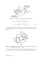
The principal stresses can be thought of as being imposed upon the surfaces
of a new cube rotated relative to the original cube by an angle θ/2, as shown in
Figure 2.10.
Now that one circle is found, two more can be found by looking into the “1”
and “3” faces. If

σ
z
is a tensile stress state of smaller magnitude than σ
y
then it
Figure 2.9 The Mohr circle for nonprincipal orthogonal stresses.
Figure 2.10 Resolving of nonprincipal stress state to a principal stress state (where there
is no shear stress in the “2,” i.e., z face).
σσ
σσ σσ
τ
σσ
σσ σσ
τ
1
2
2
3
2
2
24
24
==
+

+
−
+
==
+
−
−
+
′
′
x
xy xy
xy
y
xy xy
xy
()()
()()
©1996 CRC Press LLC
lies between σ
1
and

σ
3
and is designated
σ
2
. By looking into the 1 face, σ
2

and
σ
3
are seen, the circle for which is sho
wn in Figure 2.11 as circle 1.
Circle 2 is drawn in the same way. (Recall that in Figures 2.5, 2.7, and 2.8
only principal stresses were imposed.) The inner cube in Figure 2.10 has only
principal stresses on it. In Figure 2.11 only those principal stresses connected
with the largest circle contribute to yielding. The von Mises equation, Equation
1, suggests otherwise. (The Mohr circle embodies the Tresca yield criterion,
incidentally.) Equation 1 for principal stresses only is:
(σ
1
–
σ
2
)
2
+ (
σ
2
–

σ
3
)
2
+ (
σ
3

–
σ
1
)
2
= 2Y
2
(5)
which can be used to show that the Tresca and von Mises yield criteria are
identical when σ
2
= either
σ
1
or
σ
3
, and farthest apart (≈15%) when σ
2
lies half
way between. Experiments in yield criteria often show data lying between the
Tresca and von Mises yield criteria.
VISCO-ELASTICITY, CREEP, AND STRESS RELAXATION
Polymers are visco-elastic, i.e., mechanically they appear to be elastic under
high strain rates and viscous under low strain rates. This behavior is sometimes
modeled by arrays of springs and dashpots, though no one has ever seen them
in real polymers. Two simple tests show visco-elastic behavior, and a particular
mechanical model is usually associated with each test, as shown in Figure 2.12.
From these data of ε and σ versus time, it can be seen that the Young’s Modulus,
E (=σ/ε), decreases with time.

The decrease in E of polymers over time of loading is very different from
the behavior of metals. When testing metals, the loading rate or the strain rates
Figure 2.11 The three Mohr circles for a cube with only principal stresses applied.
©1996 CRC Press LLC
are usually not carefully controlled, and accurate data are often taken by stopping
the test for a moment to take measurements. That would be equivalent to a stress
relaxation test, though very little relaxation occurs in the metal in a short time
(a few hours).
For polymers which relax with time, one must choose a time after quick
loading and stopping, at which the measurements will be taken. Typically these
times are 10 seconds or 30 seconds. The 10-second values for E for four polymers
are given in Table 2.1.
Dynamic test data are more interesting and more common than data from
creep or stress relaxation tests. The measured mechanical properties are Young’s
Modulus in tension, E, or in shear, G, (strictly, the tangent moduli E′ and G′) and
the damping loss (fraction of energy lost per cycle of straining), Δ, of the material.
(Some authors define damping loss in terms of tan δ, which is the ratio E″/E′
where E″ is the loss modulus.) Both are strain rate (frequency, f, for a constant
amplitude) and temperature (T) dependent, as shown in Figure 2.13. The range
of effective modulus for linear polymers (plastics) is about 100 to 1 over ≈ 12
orders of strain rate, and that for common rubbers is about 1000 to 1 over ≈ 8
orders of strain rate.
The location of the curves on the temperature axis varies with strain rate, and
vice versa as shown in Figure 2.13. The temperature–strain rate interdependence,
i.e., the amount, a
T
, that the curves for E and Δ are translated due to temperature,
can be expressed by either of two equations (with varying degrees of accuracy):
Figure 2.12 Spring/dashpot models in a creep test and a stress relaxation test.
Table 2.1 Young’s Modulus for Various Materials

Solid E. Young’s Modulus
polyethylene ≈ 34,285 psi (10s modulus)
polystyrene ≈ 485,700 psi (10s modulus)
polymethyl-methacrylate ≈ 529,000 psi (10s modulus)
Nylon 6-6 ≈ 285,700 psi (10s modulus)
steel ≈ 30 × 10
6
psi (207 GPa)
brass ≈ 18 × 10
6
psi (126 GPa)
lime-soda glass ≈ 10 × 10
6
psi (69.5 GPa)
aluminum ≈ 10 × 10
6
psi (69.5 GPa)
©1996 CRC Press LLC
where ΔH is the (chemical) activation energy of the behavior in question, R is
the gas constant, T is the temperature of the test, and T
o

is the “characteristic
temperature” of the material; or
where T
s
=
T
g

+ 50°C and T
g
is the glass transition temperature of the polymer
.
1
The glass transition temperature, T
g
, is the most widely known “characteristic
temperature” of polymers. It is most accurately determined while measuring the
coefficient of thermal expansion upon heating and cooling very slowly. The value
of the coefficient of thermal expansion is greater above T
g
than belo
w. (Polymers
do not become transparent at T
g
; rather they become brittle like glassy solids,
which have short range order. Crystalline solids have long range order; whereas
super-cooled liquids have no order, i.e., are totally random.)
An approximate value of T
g
may also be mark
ed on curves of damping loss
(energy loss during strain cycling) versus temperature. The damping loss peaks
are caused by morphologic transitions in the polymer. Most solid (non “rubbery”)
polymers have 2 or 3 transitions in simple cyclic straining. For example, PVC
shows three peaks over a range of temperature. The large (or α) peak is the most
significant, and the glass transition is shown in Figure 2.14. This transition is
thought to be the point at which the free volume within the polymer becomes
greater than 2.5% where the molecular backbone has room to move freely. The

Figure 2.13 Dependence of elastic modulus and damping loss on strain rate and temper-
ature. (Adapted from Ferry, J. D., Visco-Elastic Properties of Polymers, John
Wiley & Sons, New York, 1961.)
Arrhenius a
H
RTT
T
o
: log( ) =−
⎛
⎝
⎜
⎞
⎠
⎟
Δ 11
WLF a
TT
TT
T
s
s
: log( )
.( )
(. )
=
−−
+−
886
101 6

©1996 CRC Press LLC
secondary (or β) peak is thought to be due to transitions in the side chains. These
take place at lower temperature and therefore at smaller free volume since the
side chains require less free volume to move. The third (or
γ) peak is thought to
be due to adjacent hydrogen bonds switching positions upon straining.
The glass–rubber transition is significant in separating rubbers from plastics:
that for rubber is below “room” temperature, e.g., –40°C for the tire rubber, and
that for plastics is often above. The glass transition temperature for polymers
roughly correlates with the melting point of the crystalline phase of the polymer.
The laboratory data for rubber have their counterpart in practice. For a rubber
sphere the coefficient of restitution was found to vary with temperature, as shown
in Figure 2.15. The sphere is a golf ball.
2
An example of visco-elastic transforms of friction data by the WLF equation
can be shown with friction data from Grosch (see Chapter 6 on polymer friction).
Data for the friction of rubber over a range of sliding speed are very similar in
shape to the curve of Δ versus strain rate shown in Figure 2.13. The data for µ
versus sliding speed for acrylonitrilebutadiene at 20°C, 30°C, 40°C, and 50°C
Figure 2.14 Damping loss curve for polyvinyl chloride.
Figure 2.15 Bounce properties of a golf ball.
©1996 CRC Press LLC
are shown in Figure 2.16, and the shift distance for each, to shift them to T
s
is
calculated.
i.e., the 50°C curve must be shifted by 1.51 order of 10, or by a factor of 13.2
to the left (negative log a
T
) as shown. The 40°C curve moves left, i.e., 10

0.87
, the
30°C curve remains virtually where it is, and the 20°C curve moves to the right
an amount corresponding to 10
0.86
.
When all curves are so shifted then a “master curve” has been constructed
which would have been the data taken at 29°C, over, perhaps 10 orders of 10 in
sliding speed range.
(See Problem Set question 2 f.)
DAMPING LOSS, ANELASTICITY, AND IRREVERSIBILITY
Most materials are nonlinearly elastic and irreversible to some extent in their
stress–strain behavior, though not to the same extent as soft polymers. In the
polymers this behavior is attributed to dashpot-like behavior. In metals the reason
is related to the motion of dislocations even at very low strains, i.e., some
dislocations fail to return to their original positions when external loading is
removed. Thus there is some energy lost with each cycle of straining. These losses
Figure 2.16 Example of WLF shift of data.
For this rubber, T thus T
To transform the 50 C data, log(a
gs
T
=− ° =+ =
−−
+−
°=
−
+−
=
−×

+
=−
21 29
886
101 6
88650 29
101 6 50 29
886 21
101 6 21
151
C and a
TT
TT
T
s
s
, , log( )
.( )
.
)
.( – )
.( )
.
.
.
©1996 CRC Press LLC
are variously described (by the various disciplines) as hysteresis losses, damping
losses, cyclic energy loss, anelasticity, etc. Some typical numbers for materials
are given in Table 2.2 in terms of
HARDNESS

The hardness of materials is most often defined as the resistance to penetration
of a material by an indenter. Hardness indenters should be at least three times
harder than the surfaces being indented in order to retain the shape of the indenter.
Indenters for the harder materials are made of diamonds of various configurations,
such as cones, pyramids, and other sharp shapes. Indenters for softer materials
are often hardened steel spheres. Loads are applied to the indenters such that
there is considerable plastic strain in ductile metals and significant amounts of
plastic strain in ceramic materials. Hardness numbers are somewhat convertible
to the strength of some materials, for example, the Bhn
3000
(Brinell hardness
number using a 3000 Kg load) multiplied by 500 provides a fair estimate of the
tensile strength of steel in psi (or use Bhn × 3.45 ≈TS, in MPa).
The size of indenter and load applied to an indenter are adjusted to achieve
a compromise between measuring properties in small homogeneous regions (e.g.,
single grains which are in the size range from 0.5 to 25 µm diameter) or average
properties over large and heterogeneous regions. The Brinell system produces an
indentation that is clearly visible (≈3 – 4 mm); the Rockwell system produces
indentations that may require a low power microscope to see; and the indentations
in the nano-indentation systems require high magnification microscopy to see.
For ceramic materials and metals, most hardness tests are static tests, though tests
have also been developed to measure hardness at high strain rates (referred to as
dynamic hardness). Table 2.3 is a list of corresponding or equivalent hardness
numbers for the most common systems of static hardness measurement.
Polymers and other visco-elastic materials require separate consideration
because they do not have “static” mechanical properties. Hardness testing of these
materials is done with a spring-loaded indenter (the Shore systems, for example).
An integral dial indicator provides a measure of the depth of penetration of the
Table 2.2 Values of Damping Loss,
ΔΔ

ΔΔ
for Various Materials
steel (most metals) ≈0.02 (2%)
cast iron ≈0.08
wood ≈0.03–0.08
concrete ≈0.09
tire rubber ≈0.20
Δ=
energy loss per cycle
strain energy input in applying the load
©1996 CRC Press LLC
indenter in the form of a hardness number. This value changes with time so that
it is necessary to report the time after first contact at which a hardness reading
is taken. Typical times are 10 seconds, 30 seconds, etc., and the time should be
reported with the hardness number. Automobile tire rubbers have hardness of
about 68 Shore D (10 s).
Notice the stress states applied in a hardness test. With the sphere the substrate
is mostly in compression, but the surface layer of the flat test specimen is stretched
and has tension in it. Thus one sees ring cracks around circular indentations in
brittle material. The substrate of that brittle material, however, usually plastically
deforms, often more than would be expected in brittle materials. In the case of
the prismatic shape indenters, the faces of the indenters push materials apart as
the indenter penetrates. Brittle material will crack at the apex of the polygonal
indentation. This crack length is taken by some to indicate the brittleness, i.e.,
Table 2.3 Approximate Comparison of Hardness Values
as Measured by the Most Widely Used Systems
(applicable to steel mostly)
Brinell Rockwell Vickers
3000 kg, b c e diamond
10mm 1/16” ball cone 1/8” ball pyramid

ball 100 kg f 150 kg f 60 kg f 1–120 g
10 62
↑
20 68 Έ
30 75 Έ
40 81 Έ
50 87 same as
100 60 93 Brinell
125 71 100 Έ
150 81 Έ
175 88 7 Έ
200 94 15 Έ
225 97 20 Έ
250 102 24 ↓
275 104 28 276
300 31 304
325 34 331
350 36 363
375 38 390
⎧
400 41 420
Έ 450 46 480
requires Έ 500 51 540
carbide Έ 550 55 630
ball Έ 600 58 765
Έ 650 62 810
Έ 675 63 850
Έ 700 65 940
⎩ 750 68 1025
Comparisons will vary according to the work hardening properties of mate-

rials being tested. Note that each system offers several combinations of
indenter shapes and applied loads.
©1996 CRC Press LLC