Tài liệu Advances in Database Technology- P3 docx

82
B. Gedik and L. Liu
Fig
.
4.
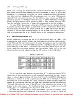
Effect of on messag-
ing cost
results using two different scenarios. In the first scenario each object reports its position
directly to the server at each time step, if its position has changed. We name this as the
naïve approach. In the second scenario each object reports its velocity vector at each
time step, if the velocity vector has changed (significantly) since the last time. We name
this as the central optimal approach. As the name suggests, this is the minimum amount
of information required for a centralized approach to evaluate queries unless there is an
assumption about object trajectories. Both of the scenarios assume a central processing
scheme.
One crucial concern is defining an optimal value for the parameter which is the
length of a grid cell. The graph in Figure 4 plots the number of messages per second
as a function of for different number of queries. As seen from the figure, both too
small and too large values of have a negative effect on the messaging cost. For smaller
values of this is because objects change their current grid cell quite frequently. For
larger values of this is mainly because the monitoring regions of the queries become
larger. As a result, more broadcasts are needed to notify objects in a larger area, of the
changes related to focal objects of the queries they are subject to be considered against.
Figure 4 shows that values in the range [4,6] are ideal for with respect to the number of
queries ranging from 100 to 1000. The optimal value of the parameter can be derived
analytically using a simple model. In this paper we omit the analytical model for space
restrictions.
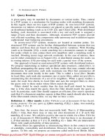
Figure 5 studies the effect of number of objects on the messaging cost. It plots
the number of messages per second as a function of number of objects for different
numbers of queries. While the number of objects is altered, the ratio of the number of
objects changing their velocity vectors per time step to the total number of objects is

kept constant and equal to its default value as obtained from Table 1. It is observed that,
when the number of queries is large and the number of objects is small, all approaches
come close to one another. However, the naïve approach has a high cost when the ratio of
the number of objects to the number of queries is high. In the latter case, central optimal
approach provides lower messaging cost, when compared to MobiEyes with EQP, but
the gap between the two stays constant as number of objects are increased. On the other
hand, MobiEyes with LQP scales better than all other approaches with increasing number
of objects and shows improvement over central optimal approach for smaller number of
Fig
.
5.
Effect of # of objects on
messaging cost
Fig
.
6.
Effect of # of objs. on
uplink messaging cost
Please purchase PDF Split-Merge on www.verypdf.com to remove this watermark.
MobiEyes: Distributed Processing of Continuously Moving Queries
83
Fig
.
7.
Effect of number of ob-
jects changing velocity vector
per time step on messaging cost
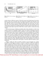
queries. Figure 6 shows the uplink component of the messaging cost. The is plotted
in logarithmic scale for convenience of the comparison. Figure 6 clearly shows that
MobiEyes with LQP significantly cuts down the uplink messaging requirement, which

is crucial for asymmetric communication environments where uplink communication
bandwidth is considerably lower than downlink communication bandwidth.
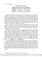
Figure 7 studies the effect of number of objects changing velocity vector per time
step on the messaging cost. It plots the number of messages per second as a function of
the number of objects changing velocity vector per time step for different numbers of
queries. An important observation from Figure 7 is that the messaging cost of MobiEyes
with EQP scales well when compared to the central optimal approach as the gap between
the two tends to decrease as the number of objects changing velocity vector per time
step increases. Again MobiEyes with LQP scales better than all other approaches and
shows improvement over central optimal approach for smaller number of queries.
Figure 8 studies the effect of base station coverage area on the messaging cost. It
plots the number of messages per second as a function of the base station coverage area
for different numbers of queries. It is observed from Figure 8 that increasing the base
station coverage decreases the messaging cost up to some point after which the effect
disappears. The reason for this is that, after the coverage areas of the base stations reach
t
o
a certain size, the monitoring regions associated with queries always lie in only one
base station’s coverage area. Although increasing base station size decreases the total
number of messages sent on the wireless medium, it will increase the average number
of messages received by a moving object due to the size difference between monitoring
regions and base station coverage areas. In a hypothetical case where the universe of
disclosure is covered by a single base station, any server broadcast will be received by
any moving object. In such environments, indexing on the air [7] can be used as an
effective mechanism to deal with this problem. In this paper we do not consider such
extreme scenarios.
Per Object Power Consumption Due to Communication
Fig. 8. Effect of base station
coverage area on messaging
cost

Fig. 9. Effect of # of queries on
per object power consumption
due to communication
So far we have considered the scalability of the MobiEyes in terms of the total number of
messages exchanged in the system. However one crucial measure is the per object power
Please purchase PDF Split-Merge on www.verypdf.com to remove this watermark.
84
B. Gedik and L. Liu
Fig. 10. Effect of on the av-
erage number of queries eval-
uated per step on a moving
object
consumption due to communication. We measure the average communication related to
power consumption using a simple radio model where the transmission path consists
of transmitter electronics and transmit amplifier where the receiver path consists of re-
ceiver electronics. Considering a GSM/GPRS device, we take the power consumption of
transmitter and receiver electronics as 150mW and 120mW respectively and we assume
a 300mW transmit amplifier with 30% efficiency [8]. We consider 14kbps uplink and
28kbps downlink bandwidth (typical for current GPRS technology). Note that sending
data is more power consuming than receiving data.
2
We simulated the MobiEyes approach using message sizes instead of message counts
for messages exchanged and compared its power consumption due to communication
with the naive and central optimal approaches. The graph in Figure 9 plots the per object
power consumption due to communication as a function of number of queries. Since
the naive approach require every object to send its new position to the server, its per
object power consumption is the worst. In MobiEyes, however, a non-focal object does
not send its position or velocity vector to the server, but it receives query updates from
the server. Although the cost of receiving data in terms of consumed energy is lower
than transmitting, given a fixed number of objects, for larger number of queries the

central optimal approach outperforms MobiEyes in terms of power consumption due to
communication. An important factor that increases the per object power consumption
in MobiEyes is the fact that an object also receives updates regarding queries that are
irrelevant mainly due to the difference between the size of a broadcast area and the
monitoring region of a query.
5.4
Computation on the Moving Object Side
In this section we study the amount of computation placed on the moving object side
by the MobiEyes approach for processing MQs. One measure of this is the number of
queries a moving object has to evaluate at each time step, which is the size of the LQT
(Recall Section 3.2).
2
In this setting transmitting costs and receiving costs
Fig. 11. Effect of the total # of
querie
s
on the avg. # of queries
evaluated per step on a moving
object
Fig. 12. Effect of the query ra-
dius on the average number of
queries evaluated per step on a
moving object
Please purchase PDF Split-Merge on www.verypdf.com to remove this watermark.
MobiEyes: Distributed Processing of Continuously Moving Queries
85
Figure 10 and Figure 11 study the effect of and the effect of the total number of
queries on the average number of queries a moving object has to evaluate at each time
step (average LQT table size). The graph in Figure 10 plots the average LQT table
size as a function of for different number of queries. The graph in Figure 11 plots the

same measure, but this time as a function of number of queries for different values of
The first observation from these two figures is that the size of the LQT table does
not exceeds 10 for the simulation setup. The second observation is that the average size
of the LQT table increases exponentially with where it increases linearly with the
number of queries.
Figure 12 studies the effect of the query radius
on the number of average queries a moving object
has to evaluate at each time step. The of
the graph in Figure 12 represents the radius factor,
whose value is used to multiply the original radius
value of the queries. The represents the av-
erage LQT table size. It is observed from the fig-
ure that the larger query radius values increase the
LQT table size. However this effect is only visible
for radius values whose difference from each other
is larger than the This is a direct result of the
definition of the monitoring region from Section 2.
Figure 13 studies the effect of the safe period
optimization on the average query processing load
of a moving object. The of the graph in Fig-
ure 12 represents the parameter, and the
represents the average query processing load of a
moving object. As a measure of query processing
6
Related Work
Evaluation of static spatial queries on moving objects, at a centralized location, is a well
studied topic. In [14], Velocity Constrained Indexing and Query Indexing are proposed
for efficient evaluation of this kind of queries at a central location. Several other indexing
structures and algorithms for handling moving object positions are suggested in the
literature [17,15,9,2,4,18]. There are two main points where our work departs from this

line of work.
Fig. 13. Effect of the safe period opti-
mization on the average query process-
ing load of a moving object
load, we took the average time spent by a moving object for processing its LQT table in
the simulation. Figure 12 shows that for large values of the safe period optimization
is very effective. This is because, as gets larger, monitoring regions get larger, which
increases the average distance between the focal object of a query and the objects in
its monitoring region. This results in non-zero safe periods and decreases the cost of
processing the LQT table. On the other hand, for very small values of like in
Figure 13, the safe period optimization incurs a small overhead. This is because the safe
period is almost always less than the query evaluation period for very small values
and as a result the extra processing done for safe period calculations does not pay off.
Please purchase PDF Split-Merge on www.verypdf.com to remove this watermark.
86
B. Gedik and L. Liu
First, most of the work done in this respect has focused on efficient indexing structures
and has ignored the underlying mobile communication system and the mobile objects.
To our knowledge, only the SQM system introduced in [5] has proposed a distributed
solution for evaluation of static spatial queries on moving objects, that makes use of the
computational capabilities present at the mobile objects.
Second, the concept of dynamic queries presented in [10] are to some extent similar
to the concept of moving queries in MobiEyes. But there are two subtle differences.
First, a dynamic query is defined as a temporally ordered set of snapshot queries in [10].
This is a low level definition. In contrast, our definition of moving queries is at end-
user level, which includes the notion of a focal object. Second, the work done in [10]
indexes the trajectories of the moving objects and describes how to efficiently evaluate
dynamic queries that represent predictable or non-predictable movement of an observer.
They also describe how new trajectories can be added when a dynamic query is actively
running. Their assumptions are in line with their motivating scenario, which is to support

rendering of objects in virtual tour-like applications. The MobiEyes solution discussed in
this paper focuses on real-time evaluation of moving queries in real-world settings, where
the trajectories of the moving objects are unpredictable and the queries are associated
with moving objects inside the system.
7
Conclusion
We have described MobiEyes, a distributed scheme for processing moving queries on
moving objects in a mobile setup. We demonstrated the effectiveness of our approach
through a set of simulation based experiments. We showed that the distributed processing
of MQs significantly decreases the server load and scales well in terms of messaging
cost while placing only small amount of processing burden on moving objects.
References
US Naval Observatory (USNO) GPS Operations. April
2003.
P. K. Agarwal, L. Arge, and J. Erickson. Indexing moving points. In PODS, 2000.
N. Beckmann, H.-P. Kriegel, R. Schneider, and B. Seeger. The R*-Tree: An efficient and
robust access method for points and rectangles. In SIGMOD, 1990.
R. Benetis, C. S. Jensen, G. Karciauskas, and S. Saltenis. Nearest neighbor and reverse
nearest neighbor queries for moving objects. In International Database Engineering and
Applications Symposium, 2002.
Y. Cai and K. A. Hua. An adaptive query management technique for efficient real-time
monitoring of spatial regions in mobile database systems. In IEEE IPCCC, 2002.
J. Hill, R. Szewczyk, A. Woo, S. Hollar, D. E. Culler, and K. S. J. Pister. System architecture
directions for networked sensors. In ASPLOS, 2000.
T. Imielinski, S. Viswanathan, and B. Badrinath. Energy efficient indexing on air. In
SIGMOD, 1994.
J.Kucera and U. Lott. Single chip 1.9 ghz transceiver frontend mmic including Rx/Tx local
oscillators and 300 mw power amplifier. MTT Symposium Digest, 4:1405–-1408, June 1999.
G. Kollios, D. Gunopulos, and V. J. Tsotras. On indexing mobile objects. In PODS, 1999.
[1]

[2]
[3]
[4]
[5]
[6]
[7]
[8]
[9]
Please purchase PDF Split-Merge on www.verypdf.com to remove this watermark.
MobiEyes: Distributed Processing of Continuously Moving Queries
87
I. Lazaridis, K. Porkaew, and S. Mehrotra. Dynamic queries over mobile objects. In EDBT,
2002.
L. Liu, C. Pu, and W. Tang. Continual queries for internet scale event-driven information
delivery. IEEE TKDE, pages 610–628,1999.
D. L. Mills. Internet time synchronization: The network time protocol. IEEE Transactions
on Communications, pages 1482–1493,1991.
D. Pfoser, C. S. Jensen, and Y. Theodoridis. Novel approaches in query processing for
moving object trajectories. In VLDB, 2000.
S. Prabhakar, Y. Xia, D. V. Kalashnikov, W. G. Aref, and S. E. Hambrusch. Query indexing
and velocity constrained indexing: Scalable techniques for continuous queries on moving
objects. IEEE Transactions on Computers, 51(10):1124–1140, 2002.
S. Saltenis, C. S. Jensen, S. T. Leutenegger, and M. A. Lopez. Indexing the positions of
continuously moving objects. In SIGMOD, 2000.
A. P. Sistla, O. Wolfson, S. Chamberlain, and S. Dao. Modeling and querying moving
objects. In ICDE, 1997.
Y. Tao and D. Papadias. Time-parameterized queries in spatio-temporal databases. In
SIGMOD, 2002.
Y. Tao, D. Papadias, and Q. Shen. Continuous nearest neighbor search. In VLDB, 2002.
[10]

[11]
[12]
[13]
[14]
[15]
[16]
[17]
[18]
Please purchase PDF Split-Merge on www.verypdf.com to remove this watermark.
DBDC: Density Based Distributed Clustering
Eshref Januzaj, Hans-Peter Kriegel, and Martin Pfeifle
University of Munich, Institute for Computer Science

{januzaj,kriegel,pfeifle}@informatik.uni-muenchen.de
Abstract. Clustering has become an increasingly important task in modern applica-
tion domains such as marketing and purchasing assistance, multimedia, molecular bi-
ology as well as many others. In most of these areas, the data are originally collected
at different sites. In order to extract information from these data, they are merged at
a central site and then clustered. In this paper, we propose a different approach. We
cluster the data locally and extract suitable representatives from these clusters. These
representatives are sent to a global server site where we restore the complete cluster-
ing based on the local representatives. This approach is very efficient, because the lo-
cal clustering can be carried out quickly and independently from each other.
Furthermore, we have low transmission cost, as the number of transmitted represent-
atives is much smaller than the cardinality of the complete data set. Based on this
small number of representatives, the global clustering can be done very efficiently.
For both the local and the global clustering, we use a density based clustering algo-
rithm. The combination of both the local and the global clustering forms our new
DBDC (Density Based Distributed Clustering) algorithm. Furthermore, we discuss
the complex problem of finding a suitable quality measure for evaluating distributed

clusterings. We introduce two quality criteria which are compared to each other and
which allow us to evaluate the quality of our DBDC algorithm. In our experimental
evaluation, we will show that we do not have to sacrifice clustering quality in order
to gain an efficiency advantage when using our distributed clustering approach.
1
Introduction
Knowledge Discovery in Databases (KDD) tries to identify valid, novel, potentially useful,
and ultimately understandable patterns in data. Traditional KDD applications require full
access to the data which is going to be analyzed. All data has to be located at that site where
it is scrutinized. Nowadays, large amounts of heterogeneous, complex data reside on differ-
ent, independently working computers which are connected to each other via local or wide
area networks (LANs or WANs). Examples comprise distributed mobile networks, sensor
networks or supermarket chains where check-out scanners, located at different stores, gather
data unremittingly. Furthermore, international companies such as DaimlerChrysler have
some data which is located in Europe and some data in the US. Those companies have var-
ious reasons why the data cannot be transmitted to a central site, e.g. limited bandwidth or
security aspects.
The transmission of huge amounts of data from one site to another central site is in some
application areas almost impossible. In astronomy, for instance, there exist several highly
sophisticated space telescopes spread all over the world. These telescopes gather data un-
E. Bertino et al. (Eds.): EDBT 2004, LNCS 2992, pp. 88–105, 2004.
© Springer-Verlag Berlin Heidelberg 2004
Please purchase PDF Split-Merge on www.verypdf.com to remove this watermark.
DBDC: Density Based Distributed Clustering
89
ceasingly. Each of them is able to collect 1GB of data per hour [10] which can only, with
great difficulty, be transmitted to a central site to be analyzed centrally there. On the other
hand, it is possible to analyze the data locally where it has been generated and stored. Ag-
gregated information of this locally analyzed data can then be sent to a central site where
the information of different local sites are combined and analyzed. The result of the central

analysis may be returned to the local sites, so that the local sites are able to put their data
into a global context.
The requirement to extract knowledge from distributed data, without a prior unification
of the data, created the rather new research area of Distributed Knowledge Discovery in Da-
tabases (DKDD). In this paper, we will present an approach where we first cluster the data
locally. Then we extract aggregated information about the locally created clusters and send
this information to a central site. The transmission costs are minimal as the representatives
are only a fraction of the original data. On the central site we “reconstruct” a global cluster-
ing based on the representatives and send the result back to the local sites. The local sites
update their clustering based on the global model, e.g. merge two local clusters to one or
assign local noise to global clusters.
The paper is organized as follows, in Section 2, we shortly review related work in the
area of clustering. In Section 3, we present a general overview of our distributed clustering
algorithm, before we go into more detail in the following sections. In Section 4, we describe
our local density based clustering algorithm. In Section 5, we discuss how we can represent
a local clustering by relatively little information. In Section 6, we describe how we can re-
store a global clustering based on the information transmitted from the local sites. Section 7
covers the problem how the local sites update their clustering based on the global clustering
information. In Section 8, we introduce two quality criteria which allow us to evaluate our
new efficient DBDC (Density Based Distributed Clustering) approach. In Section 9, we
present the experimental evaluation of the DBDC approach and show that its use does not
suffer from a deterioration of quality. We conclude the paper in Section 10.
2
Related Work
In this section, we first review and classify the most common clustering algorithms. In
Section 2.2, we shortly look at parallel clustering which has some affinity to distributed
clustering.
2.1
Clustering
Given a set of objects with a distance function on them (i.e. a feature database), an interest-

ing data mining question is, whether these objects naturally form groups (called clusters)
and what these groups look like. Data mining algorithms that try to answer this question are
called clustering algorithms. In this section, we classify well-known clustering algorithms
according to different categorization schemes.
Clustering algorithms can be classified along different, independent dimensions. One
well-known dimension categorizes clustering methods according to the result they produce.
Here, we can distinguish between hierarchical and partitioning clustering algorithms [13,
15]. Partitioning algorithms construct a flat (single level) partition of a database D of n ob-
jects into a set of k clusters such that the objects in a cluster are more similar to each other
Please purchase PDF Split-Merge on www.verypdf.com to remove this watermark.
90
E. Januzaj, H.-P. Kriegel, and M. Pfeifle
Fig. 1. Classification scheme for clustering algorithms
than to objects in different clusters. Hierarchical algorithms decompose the database into
several levels of nested partitionings (clusterings), represented for example by a dendro-
gram, i.e. a tree that iteratively splits D into smaller subsets until each subset consists of only
one object. In such a hierarchy, each node of the tree represents a cluster of D.
Another dimension according to which we can classify clustering algorithms is from an
algorithmic point of view. Here we can distinguish between optimization based or distance
based algorithms and density based algorithms. Distance based methods use the distances
between the objects directly in order to optimize a global cluster criterion. In contrast, den-
sity based algorithms apply a local cluster criterion. Clusters are regarded as regions in the
data space in which the objects are dense, and which are separated by regions of low object
density (noise).
An overview of this classification scheme together with a number of important clustering
algorithms is given in Figure 1. As we do not have the space to cover them here, we refer
the interested reader to [15] were an excellent overview and further references can be found.
2.2
Parallel Clustering and Distributed Clustering
Distributed Data Mining (DDM) is a dynamically growing area within the broader field

of KDD. Generally, many algorithms for distributed data mining are based on algorithms
which were originally developed for parallel data mining. In [16] some state-of-the-art re-
search results related to DDM are resumed.
Whereas there already exist algorithms for distributed and parallel classification and as-
sociation rules [2, 12, 17, 18, 20, 22], there do not exist many algorithms for parallel and
distributed clustering.
In [9] the authors sketched a technique for parallelizing a family of center-based data
clustering algorithms. They indicated that it can be more cost effective to cluster the data
in-place using an exact distributed algorithm than to collect the data in one central location
for clustering. In [14] the “collective hierarchical clustering algorithm” for vertically dis-
tributed data sets was proposed which applies single link clustering. In contrast to this ap-
proach, we concentrate in this paper on horizontally distributed data sets and apply a
Please purchase PDF Split-Merge on www.verypdf.com to remove this watermark.
DBDC: Density Based Distributed Clustering
91
partitioning clustering. In [19] the authors focus on the reduction of the communication cost
by using traditional hierarchical clustering algorithms for massive distributed data sets.
They developed a technique for centroid-based hierarchical clustering for high dimensional,
horizontally distributed data sets by merging clustering hierarchies generated locally. In
contrast, this paper concentrates on density based partitioning clustering.
In [21] a parallel version of DBSCAN [7] and in [5] a parallel version of k-means [11]
were introduced. Both algorithms start with the complete data set residing on one central
server and then distribute the data among the different clients.
The algorithm presented in [5] distributes N objects onto P processors. Furthermore, k
initial centroids are determined which are distributed onto the P processors. Each processor
assigns each of its objects to one of the k centroids. Afterwards, the global centroids are up-
dated (reduction operation). This process is carried out repeatedly until the centroids do not
change any more. Furthermore, this approach suffers from the general shortcoming of
k-means, where the number of clusters has to be defined by the user and is not determined
automatically.

The authors in [21 ] tackled these problems and presented a parallel version of DBDSAN.
They used a ‘shared nothing’-architecture, where several processors where connected to
each other. The basic data-structure was the dR*-tree, a modification of the R*-tree [3]. The
dR*-tree is a distributed index-structure where the objects reside on various machines. By
using the information stored in the dR*-tree, each local site has access to the data residing
on different computers. Similar, to parallel k-means, the different computers communicate
via message-passing.
In this paper, we propose a different approach for distributed clustering assuming we
cannot carry out a preprocessing step on the server site as the data is not centrally available.
Furthermore, we abstain from an additional communication between the various client sites
as we assume that they are independent from each other.
3
Density Based Distributed Clustering
Distributed Clustering assumes that the objects to be clustered reside on different sites. In-
stead of transmitting all objects to a central site (also denoted as server) where we can apply
standard clustering algorithms to analyze the data, the data are clustered independently on
the different local sites (also denoted as clients). In a subsequent step, the central site tries
to establish a global clustering based on the local models, i.e. the representatives. This is a
very difficult step as there might exist dependencies between objects located on different
sites which are not taken into consideration by the creation of the local models. In contrast
to a central clustering of the complete dataset, the central clustering of the local models can
be carried out much faster.
Distributed Clustering is carried out on two different levels, i.e. the local level and the
global level (cf. Figure 2). On the local level, all sites carry out a clustering independently
from each other. After having completed the clustering, a local model is determined which
should reflect an optimum trade-off between complexity and accuracy. Our proposed local
models consist of a set of representatives for each locally found cluster. Each representative
is a concrete object from the objects stored on the local site. Furthermore, we augment each
representative with a suitable value. Thus, a representative is a good approximation
Please purchase PDF Split-Merge on www.verypdf.com to remove this watermark.

92
E. Januzaj, H.-P. Kriegel, and M. Pfeifle
Fig. 2
.
Distributed Clustering
for all objects residing on the corresponding local site which are contained in the
around this representative.
Next the local model is transferred to a central site, where the local models are merged
in order to form a global model. The global model is created by analyzing the local repre-
sentatives. This analysis is similar to a new clustering of the representatives with suitable
global clustering parameters. To each local representative a global cluster-identifier is as-
signed. This resulting global clustering is sent to all local sites.
If a local object belongs to the of a global representative, the clus-
ter-identifier from this representative is assigned to the local object. Thus, we can achieve
that each site has the same information as if their data were clustered on a global site, to-
gether with the data of all the other sites.
To sum up, distributed clustering consists of four different steps (cf. Figure 2):
Local clustering
Determination of a local model
Determination of a global model, which is based on all local models
Updating of all local models
4
Local Clustering
As the data are created and located at local sites we cluster them there. The remaining
question is “which clustering algorithm should we apply”. K-means [11] is one of the most
commonly used clustering algorithms, but it does not perform well on data with outliers or
with clusters of different sizes or non-globular shapes [8]. The single link agglomerative
clustering method is suitable for capturing clusters with non-globular shapes, but this ap-
proach is very sensitive to noise and cannot handle clusters of varying density [8]. We used
the density-based clustering algorithm DBSCAN [7], because it yields the following advan-

tages:
DBSCAN is rather robust concerning outliers.
DBSCAN can be used for all kinds of metric data spaces and is not confined to vector
spaces.
DBSCAN is a very efficient and effective clustering algorithm.
Please purchase PDF Split-Merge on www.verypdf.com to remove this watermark.
DBDC: Density Based Distributed Clustering
93
There exists an efficient incremental version, which would allow incremental cluster-
ings on the local sites. Thus, only if the local clustering changes “considerably”, we
have to transmit a new local model to the central site [6].
We slightly enhanced DBSCAN so that we can easily determine the local model after we
have finished the local clustering. All information which is comprised within the local mod-
el, i.e. the representatives and their corresponding is computed on-the-fly during
the DBSCAN run.
In the following, we describe DBSCAN in a level of detail which is indispensable for
understanding the process of extracting suitable representatives (cf. Section 5).
4.1
The Density-Based Partitioning Clustering-Algorithm DBSCAN
The key idea of density-based clustering is that for each object of a cluster the neighbor-
hood of a given radius (Eps) has to contain at least a minimum number of objects (MinPts),
i.e. the cardinality of the neighborhood has to exceed some threshold. Density-based clus-
ters can also be significantly generalized to density-connected sets. Density-connected sets
are defined along the same lines as density-based clusters.
We will first give a short introduction to DBSCAN. For a detailed presentation of
DBSCAN see [7].
Definition 1 (directly density-reachable). An object p is directly density-reachable from
an object q wrt. Eps and MinPts in the set of objects D if
is the subset of
D

contained in the Eps-neighborhood of
q
)
(core-object condition)
Definition 2 (density-reachable). An object p is density-reachable from an object q wrt.
Eps and MinPts in the set of objects D, denoted as if there is a chain of objects
such that and is directly density-reachable from wrt.
Eps and MinPts.
Density-reachability is a canonical extension of direct density-reachability. This relation
is transitive, but it is not symmetric. Although not symmetric in general, it is obvious that
density-reachability is symmetric for objects o with Two “border ob-
jects” of a cluster are possibly not density-reachable from each other because there are not
enough objects in their Eps-neighborhoods. However, there must be a third object in the
cluster from which both “border objects” are density-reachable. Therefore, we introduce the
notion of density-connectivity.
Definition 3 (density-connected). An object p is density-connected to an object q wrt. Eps
and MinPts in the set of objects
D
if there is an object such that both, p and q are
density-reachable from o wrt. Eps and MinPts in D.
Density-connectivity is a symmetric relation. A cluster is defined as a set of density-
connected objects which is maximal wrt. density-reachability and the noise is the set of ob-
jects not contained in any cluster.
Definition 4 (cluster). Let
D
be a set of objects. A cluster C wrt. Eps and MinPts in
D
is a
non-empty subset of D satisfying the following conditions:
Maximality: and wrt. Eps and MinPts, then also

Connectivity: is density-connected to q wrt. Eps and MinPts in D.
if
Please purchase PDF Split-Merge on www.verypdf.com to remove this watermark.
94
E. Januzaj, H.-P. Kriegel, and M. Pfeifle
Definition 5 (noise). Let be the clusters wrt. Eps and MinPts in D. Then, we define
the noise as the set of objects in the database D not belonging to any cluster i.e.
noise =
We omit the term “wrt. Eps and MinPts ” in the following whenever it is clear from the
context. There are different kinds of objects in a clustering: core objects (satisfying condi-
tion 2 of definition 1) or non-core objects otherwise. In the following, we will refer to this
characteristic of an object as the core object property of the object. The non-core objects in
turn are either border objects (no core object but density-reachable from another core ob-
ject) or noise objects (no core object and not density-reachable from other objects).
The algorithm DBSCAN was designed to efficiently discover the clusters and the noise
in a database according to the above definitions. The procedure for finding a cluster is based
on the fact that a cluster as defined is uniquely determined by any of its core objects: first,
given an arbitrary object p for which the core object condition holds, the set of
all objects o density-reachable from p in D forms a complete cluster C. Second, given a clus-
ter C and an arbitrary core object C in turn equals the set (c.f. lemma 1
and 2 in
[7]).
To find a cluster, DBSCAN starts with an arbitrary core object p which is not yet clus-
tered and retrieves all objects density-reachable from p. The retrieval of density-reachable
objects is performed by successive region queries which are supported efficiently by spatial
access methods such as R*-trees [3] for data from a vector space or M-trees [4] for data from
a metric space.
5
Determination of a Local Model
After having clustered the data locally, we need a small number of representatives which

describe the local clustering result accurately. We have to find an optimum trade-off be-
tween the following two opposite requirements:
We would like to have a small number of representatives.
We would like to have an accurate description of a local cluster.
As the core points computed during the DBSCAN run contain in its Eps-neighborhood
at least MinPts other objects, they might serve as good representatives. Unfortunately, their
number can become very high, especially in very dense areas of clusters. In the following,
we will introduce two different approaches for determining suitable representatives which
are both based on the concept of specific core-points.
Definition 6 (specific core points). Let
D
be a set of objects and let be a cluster
wrt. Eps and MinPts. Furthermore, let be the set of core-points belonging to this
cluster. Then is called a complete set of specific core points of
C
iff the following
conditions are true.
There might exist several different sets which fulfil Definition 6. Each of these
sets usually consists of several specific core points which can be used to describe the
cluster C.
Please purchase PDF Split-Merge on www.verypdf.com to remove this watermark.
DBDC: Density Based Distributed Clustering
95
The small example in Figure 3a shows that if
A
is an element of the set of specific
core-points Scor, object B can not be included in Scor as it is located within the Eps-
neighborhood of
A
. C might be contained in Scor as it is not in the

Eps
-neighborhood of A.
On the other hand, if B is within Scor, A and C are not contained in Scor as they are both in
the
Eps
-neighborhood of B. The actual processing order of the objects during the DBSCAN
run determines a concrete set of specific core points. For instance, if the core-point B is vis-
ited first during the DBSCAN run, the core-points
A
and C are not included in Scor.
In the following, we introduce two local models called, (cf. Section 5.1) and
(cf. Section 5.2) which both create a local model based on the complete set of
specific core points.
5.1
Local Model:
In the case of density-based clustering, very often several core points are in the
E
ps-neighborhood of another core point. This is especially true, if we have dense clusters
and a large Eps-value. In Figure 3a, for instance, the two core points A and B are within the
Eps-
range
of each other as dist(A, B) is smaller than Eps.
Assuming core point
A
is a specific core point, i.e. than because of
condition 2 in Definition 6. In this case, object A should not only represent the objects in its
own neighborhood, but also the objects in the neighborhood of B, i.e. A should represent all
objects of In order for
A
to be a representative for the objects

we have to assign a new specific to
A
with
(cf. Figure 3a). Of course we have to assign such a specific to all specific core
points, which motivates the following definition:
Definition 7 (specific Let be a cluster wrt. Eps and MinPts. Furthermore,
let be a complete set of specific core-points. Then we assign to each an
indicating the represented area of
S
:
This specific value is part of the local model and is evaluated on the server site
to develop an accurate global model. Furthermore, it is very important for the updating proc-
ess of the local objects. The specific value is integrated into the local model of site
k as follows:
5.2
Local Model:
This approach is also based on the complete set of specific core-points. In contrast to the
previous approach, the specific core points are not directly used to describe a cluster. In-
stead, we use the number and the elements of as input parameters for a further
“clustering step” with an adapted version of k-means. For each cluster C, found by
DBSCAN, k-means yields centroids within
C
. These centroids are used as represen-
tatives. The small example in Figure 3b shows that if object
A
is a specific core point, and
In this model, we represent each local cluster by a complete set of specific core points
If we assume that we have found
n
clusters on a local site k, the local model

is formed by the union of the different sets
Please purchase PDF Split-Merge on www.verypdf.com to remove this watermark.
96
E. Januzaj, H.-P. Kriegel, and M. Pfeifle
Fig. 3
.
Local models
a)
specific core points and specific
b)
representatives by using k-means
we apply an additional clustering step by using k-means, we get a more appropriate repre-
sentative A’.
K-means is a partitioning based clustering method which needs as input parameters the
number m of clusters which should be detected within a set M of objects. Furthermore, we
have to provide m starting points for this algorithm, if we want to find m clusters. We use
k-means as follows:
Each local cluster C which was found throughout the original DBSCAN run on the
local site forms a set M of objects which is again clustered with k-means.
We ask k-means to find (sub)clusters within C, as all specific core points
together yield a suitable number of representatives. Each of the centroids found by
k-means within cluster C is then used as a new representative. Thus the number of rep-
resentatives for each cluster is the same as in the previous approach.
As initial starting points for the clustering of C with k-means, we use the set of com-
plete specific core points
6
Determination of a Global Model
Each local model consists of a set of consisting of a representative
r and an value The number m of pairs transmitted from each site k is determined
by the number n of clusters found on site k and the number of specific core-points

for each cluster as follows:
Again, let us assume that there are n clusters on a local site k. Furthermore, let
be the
centroids found by the clustering of with k-means. Let
set of objects which are assigned to the centroid
Then we assign to each
centroid
an
-range, indicating the represented area by
as follows:
Finally, the local model, describing the n clusters on site k, can be generated analogously
to the previous section as follows:
Please purchase PDF Split-Merge on www.verypdf.com to remove this watermark.
DBDC: Density Based Distributed Clustering
97
Fig. 4. Determination of a global model
a)
local clusters
b)
local representatives
c)
determina-
tion of a global model with
Each of these pairs represent several objects which are all located in i.e. the
of r. All objects contained in belongs to the same cluster. To put it an-
other way, each specific local representative forms a cluster on its own. Obviously, we have
to check whether it is possible to merge two or more of these clusters. These merged local rep-
resentatives together with the unmerged local representatives form the global model. Thus, the
global model consist of clusters consisting of one or of several local representatives.
To find such a global model, we use the density based clustering algorithm DBSCAN

again. We would like to create a clustering similar to the one produced by DBSCAN if ap-
plied to the complete dataset with the local parameter settings. As we have only access to
the set of all local representatives, the global parameter setting has to be adapted to this ag-
gregated local information.
As we assume that all local representatives form a cluster on their own it is enough to use
a of 2. If 2 representatives, stemming from the same or different lo-
cal sites, are density connected to each other wrt. and then they be-
long to the same global cluster.
The question for a suitable value, is much more difficult. Obviously,
should be greater than the E
ps
-parameter used for the clustering on the local sites.
For high values, we run the risk of merging clusters together which do not belong
together. On the other hand, if we use small values, we might not be able to detect
clusters belonging together. Therefore, we suggest that the parameter should be
tunable by the user dependent on the values of all local representatives R. If these val-
ues are generally high it is advisable to use a high value. On the other hand, if the
values are low, a small value is better. The default value which we propose is
Please purchase PDF Split-Merge on www.verypdf.com to remove this watermark.
98
E. Januzaj, H.-P. Kriegel, and M. Pfeifle
equal to the maximum value of all values of all local representatives R. This default
value is generally close to (cf. Section 9).
In Figure 4, an example for is depicted. In Figure 4a the independ-
ently detected clusters on site 1,2 and 3 are depicted. The cluster on site 1 is characterized
by two representatives R1 and R2, whereas the clusters on site 2 and site 3 are only charac-
terized by one representative as shown in Figure 4b. Figure 4c (VII) illustrates that all 4
clusters from the different sites belong to one large cluster. Figure 4c (VIII) illustrates that
an equal to is insufficient to detect this global cluster. On the other hand,
if we use an parameter equal to the 4 representatives are merged together

to one large cluster (cf. Figure 4c (IX)).
Instead of a user defined parameter, we could also use a hierarchical density
based clustering algorithm, e.g. OPTICS [1], for the creation of the global model. This ap-
proach would enable the user to visually analyze the hierarchical clustering structure for
several without running the clustering algorithm again and again. We
refine from this approach because of several reasons. First, the relabeling process discussed
in the next section would become very tedious. Second, a quantitative evaluation (cf.
Section 9) of our DBDC algorithm is almost impossible. Third, the incremental version of
DBSCAN allows us to start with the construction of the global model after the first repre-
sentatives of any local model come in. Thus we do not have to wait for all clients to have
transmitted their complete local models.
7
Updating of the Local Clustering Based on the Global Model
After having created a global clustering, we send the complete global model to all client
sites. The client sites relabel all objects located on their site independently from each other.
On the client site, two former independent clusters may be merged due to this new relabe-
ling. Furthermore, objects which were formerly assigned to local noise are now part of a glo-
bal cluster. If a local object o is in the of a representative r, o is assigned to the
same global cluster as
r
.
Figure 5 depicts an example for this relabeling process. The objects R1 and R2 are the
local representatives. Each of them forms a cluster on its own. Objects A and B have been
classified as noise. Representative R3 is a representative stemming from another site. As R1,
R2 and R3 belong to the same global cluster all Objects from the local clusters Cluster 1 and
Cluster 2 are assigned to this global cluster. Furthermore, the objects A and B are assigned
to this global cluster as they are within the
of R3,i.e.
the other hand, object C still belongs to noise as
These updated local client clusterings help the clients to answer server questions effi-

ciently, e.g. questions such as “give me all objects on your site which belong to the global
cluster 4711”.
8
Quality of Distributed Clustering
There exist no general quality measure which helps to evaluate the quality of a distribut-
ed clustering. If we want to evaluate our new DBDC approach, we first have to tackle the
problem of finding a suitable quality criterion. Such a suitable quality criterion should yield
a high quality value if we compare a “good” distributed clustering to a central clustering,
On
Please purchase PDF Split-Merge on www.verypdf.com to remove this watermark.
DBDC: Density Based Distributed Clustering
99
Fig. 5. Relabeling of the local clustering
i.e. reference clustering. On the other hand, it should yield a low value if we compare a
“bad” distributed clustering to a central clustering. Needless to say, if we compare a refer-
ence clustering to itself, the quality should be 100%. Let us first formally introduce the no-
tion of a clustering.
Definition 8 (clustering CL). be a database consisting of n objects.
Then, we call any set CL a clustering of D w.r.t. MinPts, if it fulfils the following proper-
ties:
In the following we denote by a clustering resulting from our distributed ap-
proach and by our central reference clustering. We will define two different qual-
ity criterions which measure the similarity between and We compare
the two introduced quality criterions to each other by discussing a small example.
Let us assume that we have n objects, distributed over k sites. Our
DBDC
-algorithm, as-
signs each object x, either to a cluster or to noise. We compare the result of our DBDC-
algorithm to a central clustering of the n objects using DBSCAN. Then we assign to each
object x a numerical value P (x) indicating the quality for this specific object. The overall

quality of the distributed clustering is the mean of the qualities assigned to each object.
of our distributed clustering w.r.t. P is computed as follows:
The crucial question is “what is a suitable object quality function?”. In the following two
subsections, we will discuss two different object functions P.
Definition 9 (distributed clustering quality . Let be a database
consisting of n objects. Let P be an object quality function Then the quality
of our distributed clustering w.r.t. P is computed as follows:
The crucial question is “what is a suitable object quality function?”. In the following two
subsections, we will discuss two different object functions P.
Please purchase PDF Split-Merge on www.verypdf.com to remove this watermark.
100
E. Januzaj, H.-P. Kriegel, and M. Pfeifle
8.1
First Object Quality Function
Obviously, P(x) should yield a rather high value, if an object x together with many other
objects is contained in a distributed cluster and a central cluster In the case of density-
based partitioning clustering, a cluster might consist of only MinPts elements. Therefore,
the number of objects contained in two identical clusters might be not higher than MinPts.
On the other hand, each cluster consists of at least MinPts elements. Therefore, asking for
less than MinPts elements in both clusters would weakening the quality criterion unneces-
sarily.
If x is included in a distributed cluster but is assigned to noise by the central cluster-
ing, the value of P(x) should be 0. If x is not contained in any distributed cluster, i.e. it is
assigned to noise, a high object quality value requires that it is also not contained in a central
cluster. In the following, we will define a discrete object quality function which assigns
either 0 or 1 to an object x, i.e. or
The main advantage of the object quality function is that it is rather simple because it
yields only a boolean return value, i.e. it tells whether an object was clustered correctly or
falsely. Nevertheless, sometimes a more subtle quality measure is required which does not
only assign a binary quality value to an object. In the following section, we will introduce a

new object quality function which is not confined to the two binary quality values 0 and 1.
This more sophisticated quality function can compute any value in between 0 and 1 which
much better reflects the notion of “correctly clustered”.
8.2
Second Object Quality Function
The main idea of our new quality function is to take the number of elements which were
clustered together with the object x during the distributed and the central clustering into con-
sideration. Furthermore, we decrease the quality of x if there are objects which have been
clustered together with x in only one of the two clusterings.
Definition 11 (continuous object quality
Let and let
be a central and
a distributed cluster. Then we define an object quality function as follows:
Definition 10 (discrete object quality
and let
be two cluster. Then
we can define an object quality function w.r.t. to a quality parameter
as
follows:
Please purchase PDF Split-Merge on www.verypdf.com to remove this watermark.
DBDC: Density Based Distributed Clustering
101
Fig. 6. Used test data sets a) test data set A
b)
test data set B
c)
test data set
C
9
Experimental Evaluation

We evaluated our DBDC-approach based on three different 2-dimensional point sets
where we varied both the number of points and the characteristics of the point sets. Figure
6 depicts the three used test data sets A (8700 objects, randomly generated data/cluster), B
(4000 objects, very noisy data) and C (1021 objects, 3 clusters) on the central site. In order
to evaluate our DBDC-approach, we equally distributed the data set onto the different client
sites and then compared DBDC to a single run of DBSCAN on all data points. We carried
out all local clusterings sequentially. Then, we collected all representatives of all local runs,
and applied a global clustering on these representatives. For all these steps, we always used
the same computer. The overall runtime was formed by adding the time needed for the glo-
bal clustering to the maximum time needed for the local clusterings. All experiments were
performed on a Pentium III/700 machine.
In a first set of experiments, we consider efficiency aspects, whereas in the following
sections we concentrate on quality aspects.
9.1
Efficiency
In Figure 7, we used test data sets with varying cardinalities to compare the
overall runtime of our DBDC-algorithm to the runtime of a central clustering. Furthermore,
we compared our two local models w.r.t. efficiency to each other. Figure 7a shows that our
DBDC
-approach outperforms a central clustering by far for large data sets. For instance, for
a point set consisting of 100,000 points, both DBDC approaches, i.e. and
outperform the central DBSCAN algorithm by more than one order of
magnitude independent of the used local clustering. Furthermore, Figure 7a shows that the
local model for can more efficiently be computed than the local model for
Figure 7b shows that for small data sets our DBDC-approach is slightly slower than the
central clustering approach. Nevertheless, the additional overhead for distributed clustering
is almost negligible even for small data sets.
In Figure 8 it is depicted in what way the overall runtime depends on the number of used
sites. We compared DBDC based on to a central clustering with DBSCAN.
Our experiments show that we obtain a speed-up factor which is somewhere between

and This high speed-up factor is due to the fact that DBSCAN has a runtime com-
plexity somewhere between O(nlogn)
and when using a suitable index structure, e.g.
an R*-tree
[3].
Please purchase PDF Split-Merge on www.verypdf.com to remove this watermark.