Tài liệu Pricing communication networks P7 docx
Bạn đang xem bản rút gọn của tài liệu. Xem và tải ngay bản đầy đủ của tài liệu tại đây (275.65 KB, 33 trang )
Part C
Pricing
Pricing Communication Networks: Economics, Technology and Modelling.
Costas Courcoubetis and Richard Weber
Copyright
2003 John Wiley & Sons, Ltd.
ISBN: 0-470-85130-9
7
Cost-based Pricing
This chapter is about prices that are directly related to cost. We begin with the
problem of finding cost-based prices that are fair or stable under potential competition
(Sections 7.1 –7.2). We look for types of prices that can protect an incumbent against entry
by potential competitors, or against bypass by customers who might find it cheaper to supply
themselves. We explain the notions of subsidy-free and sustainable prices. Such prices are
robust against bypass. Similar notions are addressed by the idea of the second-best core. The
aim now differs from that of maximizing economic efficiency. We see that Ramsey prices,
which are efficient subject to the constraint of cost recovery, may fail sustainability tests.
In Section 7.3 we take a different approach and look at practical issues of constructing
cost-based prices. Now we emphasize necessary and simplicity. Prices are to be computed
from quantities that can be easily measured and for which accounting data is readily
available. An approach that has found much favour with regulators is that of Fully
Distributed Cost pricing (FDC). This is a top-down approach, in which costs are attributed
to services using the firm’s existing cost accounting records. It ignores economic efficiency,
but has the great advantage of simplicity.
Section 7.3.5 concerns the Long-Run Incremental Cost approach (LRIC). This is a
bottom-up approach, in which the costs of the services are computed using an optimized
model for the network and the service production technologies. It can come close to
implementing subsidy-free prices. We compare FDC and LRIC in Section 7.4, from the
viewpoint of the regulator, who wishes to balance the aims of encouraging efficiency and
competition, and of the monopolist who would like to set sustainable prices. The regulator
may prefer the accounting-based approach of FDC pricing because it is ‘automatic’ and
auditable. However, it may obscure old and inefficient production technology or the fact
that the network has been wrongly dimensioned. These problems can be remedied by the
LRIC approach, but it is more costly to implement.
Flat rate pricing is the subject of Section 7.5. In this type of pricing a customer’s charge
does not depend on the actual quantity of services he consumes. Rather, he is charged the
average cost of other customers in the same customer group. We discuss the incentives that
such a scheme provides and their effects on the market.
7.1 Foundations of cost-based pricing
In Chapters 5 and 6 we considered the problem of pricing in a context in which social
welfare maximization is the overall aim. We posed optimization problems with unique
Pricing Communication Networks: Economics, Technology and Modelling.
Costas Courcoubetis and Richard Weber
Copyright
2003 John Wiley & Sons, Ltd.
ISBN: 0-470-85130-9
164 COST-BASED PRICING
solutions, each achieved by unique sets of prices. However, welfare maximization is not
the only thing that matters. A firm’s prices must ensure that it is profitable, or at least
that it covers its costs. Cost-based pricing focuses on this consideration. Unfortunately, a
fundamental difficulty in defining cost-based prices is that services are usually produced
jointly. A large part of the total cost is a common cost, which can be difficult to
apportion rationally amongst the different services. One can think of several ways to
do it. So although cost-based prices may reasonably be expected to satisfy certain
necessary conditions, they differ from welfare-maximizing prices in that they are usually
not unique.
One necessary condition that cost-based prices ought reasonably to satisfy is that of
fairness. Some customers should not find themselves subsidizing the cost of providing
services to other customers. If so, these customers are likely to take their business elsewhere.
This motivates the idea of subsidy-free prices. A second reasonable necessary condition is
that prices should be defensive against competition, discouraging the entry of competitors
who by posting lower prices could capture market share. This motivates the idea of
sustainable prices. If prices do not reflect actual costs or they hide costs of inefficient
production then they invite competition from other firms. Since customers will choose the
provider from whom they believe they get the best deal, a game takes place amongst
providers, as they seek to offer better deals to customers by deploying different cost
functions and operating at different production levels. Prices must be subsidy-free and
sustainable if they are to be stable prices, that is, if they are to survive the competition in
this game.
Interestingly, the set of necessary conditions that we might like to impose on prices can
be mutually incompatible. They can also be in conflict with the aim of maximizing social
welfare maximization, since they restrict the feasible set of operating points, sometimes
reducing it to a single point.
7.1.1 Fair Charges
Consider the problem of a single provider who wishes to price his services so that they
cover their production cost and are fair in the sense that no customer feels he is subsidizing
others. Unfair prices leave him susceptible to competition from another provider, who has
the same costs, but charges fairly. Customers might even become producers of their own
services.
Let N Df1; 2;:::;ng denote a set of n customers, each of whom wishes to buy some
services. For T that is a subset N,andletc.T / denote the minimal cost that could by
incurred by a facility that is optimized to provide precisely the services desired by the set
of customers T . We call this the stand-alone cost of providing services to the customers in
T . Assume that because of economies of scale and scope this cost function is subadditive.
That is, for all disjoint sets T and U ,
c.T [ U/ Ä c.T / C c.U/ (7.1)
In the terminology of cooperative games, c.Ð/ is called a characteristic function.
The service provider wants to share the total cost of providing the services amongst the
customers in a manner that they think is fair. Suppose he charges them amounts c
1
;:::;c
n
.
Let us further suppose that he exactly covers his cost, and so
P
i2N
c
i
D c.N/. The charges
are said to subsidy free if they satisfy the following two tests:
FOUNDATIONS OF COST-BASED PRICING 165
ž The charge made to any subset of customers is no more than the stand-alone cost of
providing services to those customers,
X
i2T
c
i
Ä c.T /; for all T Â N (7.2)
ž The charge made to any subset of customers is at least the incremental cost of providing
services to those customers,
X
i2T
c
i
½ c.N/ c.N n T /; for all T Â N (7.3)
The reason these conditions are interesting is that if either (7.2) or (7.3) is violated, then
a new entrant can attract dissatisfied customers. If (7.2) is violated, then a firm producing
only services for T and charging only c.T / could lure away these customers. Similarly, if
(7.3) is violated, then a firm producing only the services needed by N n T could charge less
for these services than the incumbent firm. This happens because the incumbent uses part
of the revenue obtained from selling services to N n T to pay for some of the cost of the
services wanted by T . Next, we investigate certain variations and refinements of the above
concepts.
7.1.2 Subsidy-free, Support and Sustainable Prices
Let reformulate the ideas of the previous section to circumstances in which charges are
computed from prices. Suppose that a set of n services is N Df1;:::;ng and an incumbent
firm sells service i in quantity x
i
,atpricep
i
, for a total charge of p
i
x
i
. Suppose that x
i
is given and does not depend on p D . p
1
;:::;p
n
/. We call p a subsidy-free price if it
satisfies the two tests
X
i2T
p
i
x
i
Ä c.T /; for all T Â N (7.4)
X
i2T
p
i
x
i
½ c.N / c.N n T /; for all T Â N (7.5)
Inequalities (7.4) and (7.5) are respectively the stand-alone test and incremental-cost test.
They have natural interpretation similar to (7.2) and (7.3). For instance, if (7.4) is violated
then a new firm could set up to produce only the services in T and sell these at lower
prices than the incumbent. Note that, by putting T D N , these tests imply
P
i
p
i
x
i
D c.N/.
Thus the producer must operate with zero profit. Also, prices must be above marginal cost;
to see this, consider the set T Dfig, imagine that x
i
is small and apply the incremental
cost test.
Example 7.1 (Subsidy-free prices may not exist) Consider a network offering voice and
video services. The cost of the basic infrastructure that is common to both services is 10
units, while the incremental cost of supplying 100 units of video service is 2 units and
the incremental cost of supplying 1000 units of voice is 1 unit. To be subsidy-free, the
revenues r
1
.100/ and r
2
.1000/ that are obtained from the video and the voice services
must satisfy
2 Ä r
1
.100/ Ä 12; 1 Ä r
2
.1000/ Ä 11; r
1
.100/ C r
2
.1000/ D 13
166 COST-BASED PRICING
Thus, assuming that there is enough demand for services, possible prices are 0:006 units
per voice service and 0:07 units per video service. Note that such prices are not unique
and they may not even exist for general cost functions. Suppose three services are pro-
duced in unit quantities with a symmetric cost function that satisfies (7.1). Let c.fi g/ D 2:5,
c.fi; j g/ D 3:5, and c.fi; j; kg/ D 5:5, where i; j; k are distinct members of f1; 2; 3g.Then
we must have 2 Ä p
i
Ä 2:5, for i D 1; 2; 3, but also p
1
C p
2
C p
3
D 5:5. So there
are no subsidy-free prices. The problem is that economies of scope are not increasing, i.e.
c.fi; j; kg/ c.fi; j g/>c.fi; j g/ c.fig/.
How can one determine if (7.4) and (7.5) are met in practice? Assume that a firm posts its
prices and makes available its cost accounting records for the services. It may be possible
to check (7.5) by computing and then summing the incremental costs of each service in
T (though this only approximates the incremental cost of T because we neglect common
cost that is directly attributable to services in T ). Condition (7.4) is hard to check, as it
imagines building from scratch a new facility that is specialized to produce the services in
the set T . This cost cannot in general be derived from the cost accounting information of
the firm which produces the larger set of services N . In practice, one tries to approximate
c.T /, as well as possible given the available information.
There is another possible problem with the above tests. Although individual outputs may
pass the incremental cost test, combinations of outputs may not. For example, suppose
N Df1; 2; 3g. It is possible that the incremental cost test can be satisfied for every single
good, i.e. for T Dfig,foralli, but not for T Df2; 3g. This could happen if there is a fixed
common cost associated with services 2 and 3, in addition to their individual incremental
costs, and each such service is priced at its incremental cost. Thus, the tests can be difficult
to verify in practice.
In defining subsidy-free prices we assumed that services are sold in large known
quantities (the x
i
s in (7.4) and (7.5)) using uniform prices, as happens when incumbent
communications firms supply the market. In practice, individual customers consume small
parts of each x
i
and a coalition of customers may feel that it can ‘self-produce’ its service
requirements at lower cost. In this case, it is reasonable to require (7.2) and (7.3). Clearly,
such a ‘consumer subsidy-free’ price condition imposes restrictions on the cost function. For
instance, imagine a single service has a cost function with increasing average cost. Selling
the service at its average cost price violates (7.3) if individual customers request less than
the total that is produced, although (7.4) and (7.5) are trivially satisfied for N Df1g.An
appropriate definition is the following. Let us now write c.x/ as the cost of providing
services in quantities .x
1
;:::;x
n
/. We say the vector p is a support price for c at x if it
satisfies the two conditions
X
i2N
p
i
y
i
Ä c.y/; for all y Ä x (7.6)
X
i2N
p
i
z
i
½ c.x/ c.x z/; for all z Ä x (7.7)
Note these imply
P
i2N
p
i
x
i
D c.x/. We can compare them to (7.2) and (7.3). For example,
(7.6) implies that one cannot produce some of the demand for less than it is sold. They
imply (7.4) and (7.5) (but are more general since they deal with arbitrary sub-quantities of
the vector x, instead of looking just at subsets of service types), and hence a support price
has all the nice fairness properties mentioned above. A last concern is whether such prices
FOUNDATIONS OF COST-BASED PRICING 167
are achievable in the market, where demand is a function of price. Suppose p is the vector
of support prices for x and, moreover, x is precisely the quantity vector that is demanded
at price p. We call such prices anonymously equitable prices. Clearly, if they exist, these
have a very good theoretical claim for being an intelligent choice of cost-based prices.
If prices affect demand
By allowing demand to depend upon price, we introduce subtle complications. Customers
may feel badly treated even if the incremental cost test in (7.7) is passed. For example,
if two services are substitutes then introducing one of them as a new service can reduce
the demand for the other and the revenue it produces. Prices may have to increase if we
are still to cover costs and this could mean that the price of the pre-existing service has
to increase. This runs counter to what we expect: that adding a new service should allow
prices of pre-existing services to decrease because of economies of scope in facility and
equipment sharing. If the prices of pre-existing services increase then customers of these
services will feel that they are subsidizing the cost of the new service.
To see this, let T be a subset of N, and define p
0
i
D1, i 2 T ,and p
0
i
D p
i
, i 62 T .
Thus, under price vector p
0
we do not sell any of the services in T (because their prices
are infinite). If services in T are substitutes for those in N n T , then we can have, (recalling
p
0
i
D p
i
for i 2 N n T ),
X
i2N nT
p
0
i
x
i
. p
0
/>
X
i2N nT
p
i
x
i
. p/
i.e. when p
0
is replaced by p, the introduction of services in T reduces the demand for (and
revenue earned from) services in N n T . Noting that
P
i2N nT
p
i
x
i
. p/ D
P
i2N
p
i
x
i
. p/
P
i2T
p
i
x
i
. p/, we see that it is possible for c.Ð/ to be such that
X
i2T
p
i
x
i
. p/>c.x. p// c.x. p
0
// >
X
i2N
p
i
x
i
. p/
X
i2N nT
p
0
i
x
i
. p
0
/
Here the incremental cost test (7.7) is passed (by the left hand inequality), but net additional
revenue does not cover additional costs (the right hand inequality). Thus, the additional
costs must be covered (at least in part) by increasing the charges levied on customers who
were happy when only services in N n T were offered, rather than only making charges to
customers who purchase services in T . These former set of customers may feel that they
are subsidizing the later set of customers, and that these new services decrease the overall
efficiency of the system. We conclude that, as a matter of fairness between customers, the
second test condition (7.7) should take account of demand, and reason in terms of the net
incremental revenue produced by an additional service, taking account of the reduction of
revenue from other services. In other words, services are fairly priced if when service i is
offered at price p
i
the customers of the other services feel that they benefit from service i.
They are happy because the prices of the services they want to buy decrease. This is called
the net incremental revenue test. Let us look at an example.
Example 7.2 (Net incremental revenue test) Suppose a facility costs C and there is no
variable cost. It initially produces a single service 1 in quantity x
1
D a at price p
1
D C=a.
Then, a new service is added, at no extra cost, and at a price p
2
that is just a little more
than 0. As a result, demand for service 2 increases at the expense of demand for service
1. To cover the cost, p
1
must increase, making even more customers switch to service 2.
168 COST-BASED PRICING
At the end, suppose that an equilibrium is reached where p
1
D 10C=a, x
1
D 0:1a and
x
2
D 0:9a C b. Note that, by our previous definition, these prices are subsidy-free, and
(almost) all the revenue is collected by charging for service 1. These customers (the ones
left using service 1) are right to complain that they subsidize service 2, since they see their
prices increase after the addition of the new service. Indeed, choosing such a low price
for service 2 results in an overall revenue reduction if prices of existing services are not
allowed to increase. A fair price would be to choose p
2
in such a way that the overall
net revenue (keeping the other prices, i.e. p
1
, fixed) would increase. Then, the zero profit
condition may be achieved by reducing the other prices and hence benefiting the customers
of the other services. In our example, suppose that by setting p
2
D p
1
and keeping p
1
at
its initial value, x
1
becomes a=2andx
2
D a=2 C b=2. In other words, half the customers
of service 1 find service 2 to suit them better at the same price, and so switch. There are
also new customers that like to use service 2 at that price. Then the net revenue increase
becomes p
1
b=2 > 0; so it is possible to decrease p
1
and allow customers of service 1 to
benefit from the addition of service 2.
Finally, consider a model of potential competition. Imagine an incumbent firm sets prices
to cover costs at the demanded quantities, i.e.
X
i2N
p
i
x
i
. p/ ½ c.x . p// (7.8)
Suppose a competitor having the same cost function as the incumbent tries to take away
part of the incumbent’s market by posting prices p
0
which are less for at least one service.
Suppose x
E
. p; p
0
/ is the demand for the services provided by the new entrant when he
and the incumbent post prices p
0
and p respectively. Suppose that there is no p
0
and x
0
such that
X
i2N
p
0
i
x
0
i
½ c.x
0
/; and p
0
i
< p
i
for some i ; and x
0
Ä x
E
. p; p
0
/ (7.9)
That is, there is no way that the potential entrant can post prices that are less than the
incumbent’s for some services and then serve all or part of the demand without incurring
loss. Prices satisfying this condition are called sustainable prices.Wehaveyetonemore
‘fairness test’ by which to judge a set of prices.
The above model motivates the use of sustainable prices in contestable markets. A
market is contestable when low cost ‘hit-and-run’ entry and exit are possible, without
giving enough time to the incumbent to react and adjust his prices or quantities he
sells. Such low barrier to entry is realized by using new technologies such as wireless,
or when the regulator prescribes that network elements can be leased from incumbents
at cost.
In the idea of sustainable prices we again see that price stability is related to efficiency.
If prices are sustainable, a new entrant cannot take away market share if his cost function
is greater than that of the incumbent. Hence sustainable prices discourage inefficient entry.
However, if a new entrant is more efficient than the incumbent, and so has a smaller
cost function, then he can always take away some of the incumbent’s market share by
posting lower prices. Thus an incumbent cannot post sustainable prices if he operates with
inefficient technologies.
It can be shown that for his prices to be sustainable, an incumbent firm must fulfil a
minimum of three necessary conditions:
FOUNDATIONS OF COST-BASED PRICING 169
1. He must operate with zero profits.
2. He must be a natural monopoly (exhibit economies of scale) and produce at minimum
cost.
3. His prices for all subsets of his output must be subsidy free, i.e. fulfil the stand-alone
and incremental cost tests.
The last remark provides one more motivation to use the subsidy-free price tests to detect
potential problems with a given set of prices.
Ramsey prices
Unfortunately, there is no straightforward recipe for constructing sustainable prices.
Constructing socially optimal prices that are sustainable is even harder. However, under
conditions that are frequently encountered in communications, Ramsey prices can be
sustainable. Recall that Ramsey prices maximize social welfare under the constraint of
recovering cost. Again we see a connection between competition and social efficiency: in
a contestable market, i.e. under potential competition, incumbents will be motivated to use
prices that maximize social efficiency with no need of regulatory intervention.
However, Ramsey prices are not always sustainable. They are certainly not sustainable
if any service, say service 1, is priced below its marginal cost and there are economies of
scale. To see this, note that revenue from service 1 does not cover its own incremental cost
since by concavity of the cost function x
1
p
1
< x
1
@c=@ x
1
< c.x/ c..0; x
2
;:::;x
n
//.So
a supplier who competes on the same set of services and with the same cost function can
more than cover his costs by electing not to produce service 1. After doing this, he can
slightly lower the prices of all the services that are priced above their marginal costs, so as
to obtain all that demand for himself and yet still cover his costs.
Example 7.3 (Ramsey prices may not be sustainable) Whether or not Ramsey prices
are sustainable can depend on how services share fixed costs, i.e., on the economies of
scope. Consider a market in which there are customers for two services. The producer’s
cost function and demand functions for the services are
c.x
1
; x
2
/ D 25x
1=2
1
C 20x
1=2
2
C F ; x
1
. p/ D x
2
. p/ D
10
4
.10 C p/
2
The Ramsey prices are shown in Table 7.1. When the fixed cost F is 6 the Ramsey prices
are not sustainable even though they exceed marginal cost. The revenue from service 2 is
169:45 and this is enough to cover the sum of its own variable cost and the entire fixed
cost, a total of 162:76. This means that a provider can offer service 2 at a price less than the
Ramsey price of 2:76 and still cover his costs. In fact, he can do this for any price greater
than 2:62. However, if the fixed cost is 30 this is now great enough that it is impossible to
cover costs by providing just one of the services alone at a lower price.
1
Hence, in this case,
the Ramsey prices are sustainable. The lesson is that Ramsey prices may be sustainable if
all services are priced above marginal cost and the economies of scope are great enough.
1
The other possibility for a new entrant is to provide both services at lower prices. But it is impossible to lower
both prices and still cover costs. If all prices are lower the consumer surplus must increase. Since we require
the producer surplus to remain nonnegative, and it was zero at our Ramsey prices, this would imply that the
social welfare — which is the sum of consumer and producer surpluses — would increase; this means we could
not have been at the Ramsey solution.
170 COST-BASED PRICING
Table 7.1 Ramsey prices may or may not be sustainable
F D 6FD 30
i D 1iD 2iD 1i=2
Ramsey price, p
i
3.18 2.76 3.46 2.64
Demand, x
i
57.58 61.44 55.18 58.96
Marginal cost 1.65 1.28 1.68 1.30
Revenue, x
i
p
i
183.02 169.45 191.02 178.26
Variable cost 189.70 156.76 185.71 153.57
Variable cost C F 195.70 162.76 215.71 183.57
To show how the existence of common cost plays a vital role in the sustainability of
Ramsey prices, we can construct a simple example out of Figure 5.5.
Example 7.4 (Common cost and sustainability of Ramsey prices) Suppose that two
services are produced with same stand-alone cost function A C bx. First, consider the
case in which there is no economy of scope, and hence the total cost is the sum
of the stand-alone cost functions. Since both services are produced at equal quantities
x
i
D x
j
D x we have x. p
i
C p
j
/ D 2. A C bx/ which implies xp
i
< A C bx < xp
j
.
But A C bx is the stand-alone cost for service j, which violates the sustainability
conditions.
Now suppose that there are economies of scope and the fixed cost A is common to both
services. Then x. p
i
C p
j
/ D AC2bx, and since p
i
> b we obtain xp
j
Cbx < AC2bx.This
implies xp
j
< A C bx, which is the stand-alone cost for service j. Hence, the existence of
common cost is vital for Ramsey prices to be sustainable. Observe that, in this particular
case, any amount of common cost, A, will make Ramsey prices sustainable. In general, as
suggested by Example 7.3, large values of A ensure sustainability.
7.1.3 Shapley Value
Let us now leave the subject of prices and return to the simple model at the start of the
chapter, in which cost is to be fairly shared amongst n customers. The provider’s charging
algorithm could be coded in a vector function which divides c.N / as .c
1
;:::;c
n
/ D
1
.N /;:::;
n
.N /
Ð
. Let us suppose that .T / is defined for an arbitrary subset T Â N ,
and codes the way he would divide the cost of c.T / amongst the members of the subset
T if he were to provide services to only this subset of customers. Clearly, .fig/ D c.fig/
being the stand-alone cost for serving only customer i.
Suppose that T Â N and i; j are distinct members of T .If
j
.T /
j
.T nfig/>0,
then customer j pays more than he would pay if customer i were not being served. He
might argue this was unfair, unless customer i can counter-argue that he is at least as
disadvantaged because of customer j. But then if customer i is not to feel aggrieved then
he must see similarly that customer j is at least as much disadvantaged. Putting this all
together requires
i
.T /
i
.T nfjg/ D
j
.T /
j
.T nfig/ (7.10)
On the other hand, if
j
.T /
j
.T nfig/<0, then customer j is better off because
customer i is also being served. Customer i might feel aggrieved unless he benefits at
least as much from the fact that customer j is present. But then customer j will feel
FOUNDATIONS OF COST-BASED PRICING 171
aggrieved unless he benefits at least as much from customer i’s presence. So again, we
must have (7.10).
Surprisingly, there is only one function which satisfies (7.10) for all T Â N and
i; j 2 T . It is called the Shapley value, and its value for player i is the expected incremental
cost of providing his service when provision of the services accumulates in random order.
It is best to illustrate this with an example.
Example 7.5 (Sharing the cost of a runway) Suppose three airplanes A, B, C share a
runway. These planes require 1, 2 and 3 km to land. So a runway of 3 km must be built.
How much should each pay? We take their requirements in the six possible orders. Cost is
measured in units per kilometer.
Adds cost
Order ABC
A, B, C 111
A, C, B 102
B, A, C 021
B, C, A 021
C, A, B 003
C, B, A 003
Total 2511
So they should pay for 2=6, 5=6 and 11=6 km, respectively.
Note that we would obtain the same answer by a calculation based on sharing common
cost. The first kilometer is shared by all three and so its cost should be allocated
as .1=3; 1=3; 1=3/. The second kilometer is shared by two, so its cost is allocated as
.0; 1=2; 1=2/. The last kilometer is used only by one and so its cost is allocated as
.0; 0; 1/. The sum of these vectors is .2=6; 5=6; 11=6/. This happens generally. Suppose
each customer requires some subset of a set of resources. If a particular resource is required
by k customers, then (under the Shapley value paradigm) each will pay one-kth of its cost.
The intuition behind the Shapley value is that each customer’s charge depends on the
incremental cost for which he is responsible. However, it is subtle, in that a customer is
charged the expected extra cost of providing his service, incremental to the cost of first
providing services to a random set of other customers in which each other customer is
equally to appear or not appear.
The Shapley value is also the only cost sharing function that satisfies four axioms, namely,
(1) all players are treated symmetrically, (2) those whose service costs nothing are charged
nothing, (3) the cost allocation is Pareto optimal, and (4) the cost sharing of a sum of costs
is the sum of the cost sharings of the individual costs. For example, the cost sharing of
an airport runway and terminal is the cost sharing of the runway plus the cost sharing of
the terminal. The Shapley value also gives answers that are consistent with other efficiency
concepts such as Nash equilibrium.
The Shapley value need not satisfy the stand-alone and incremental cost tests, (7.2) and
(7.3). However, one can show that it does so if c is submodular,i.e.if
c.T \ U / C c.T [ U / Ä c.U / C c.T /; for all T ; U Â N (7.11)
The reader can prove this by looking at the definition of the Shapley value and using
an equivalent condition for submodularity, that taking the members of N in any order,
172 COST-BASED PRICING
say i; j; k;:::;`,wemusthave
c.fig/ ½ c.fi; jg/ c.f j g/ ½ c.fi; j; kg/ c.f j; kg/ ½ ÐÐÐ ½ c.N / c.N fig/
Note that choosing T and U disjoint shows that submodularity is consistent with c.Ð/ being
subadditive, i.e. (7.1).
7.1.4 The Nucleolus
The Shapley value has given us one way to allocate charges and it is motivated by a nice
story of argument and counterargument. However, there are other stories we can tell. Let
us call c an imputation of cost (i.e., an assignment of cost) if
X
i2N
c
i
D c.N / and c
i
Ä c.fig/; for all i
That is, the provider exactly covers his costs and no customer is charged more than his
stand-alone cost.
We now suggest a reasonable condition that the imputation c should satisfy. Suppose
that for all imputations c
0
and subsets T Â N such that
P
i2T
c
0
i
<
P
i2T
c
i
there exists
some U Â N (not necessarily disjoint from T ) such that
X
i2U
c
0
i
>
X
i2U
c
i
and
X
i2U
c
0
i
c.U />
X
i2T
c
i
c.T /
So if a set of customers T prefers an imputation c
0
(because their total charge is less), then
there is always some other set of customers U who can object because
ž under c
0
the total charge they pay is more, i.e.
P
i2U
c
0
i
>
P
i2U
c
i
,and
ž they pay under c
0
a greater increment over their stand-alone cost, c.U /,thanT pays
under c over its stand-alone cost, c.T /.
so U argues that T should not have a cost-reduction at U’s expense.
Then c is said to be in the nucleolus (of the coalitional game). It is a theorem that
the nucleolus always exists and is a single point. Thus the nucleolus is a good candidate
for being the solution to the cost-sharing problem. In the runway-sharing example, the
nucleolus is .1=2; 1; 3=2/. Note that it is not the same as the Shapley cost allocation of
c D .2=6; 5=6; 11=6/. The fact that c is not the nucleolus can be seen by taking T DfB; Cg
and c
0
D .3=6; 5=6; 10=6/. There is no U that can object to this.
What would have happened if we had simultaneously tried to satisfy the conditions of
both the nucleolus and Shapley ‘stories’? The answer is that there would be no solution.
The lesson in this is that ‘fair’ allocations of cost cannot be uniquely-defined. There are
many definitions we might choose, and our choice should depend on the sort of unfairnesses
that we are trying to avoid. We now end this section with a final story.
7.1.5 The Second-best Core
Thus far we have mostly been allocating cost without paying attention to the benefit that
customers obtain. Surely, it is fair that a customer who benefits more should pay more. We
end this section with a cost sharing problem that takes account of the benefit that customers
obtain.
FOUNDATIONS OF COST-BASED PRICING 173
S
1
2
N
coalition
Figure 7.1 The second-bestž core. The monopolist fixes p s.t. p
>
x c.x/ ½ 0, where x is the
aggregate demand, x D
P
N
iD1
x
i
. p/,andc.x / is the cost of producing x. The entrant targets a
subset of customers S who he wishes to woo. He chooses p
S
s.t. . p
S
/
>
x
S
c.x
S
/ ½ 0, where
x
S
D
P
i2S
x
i
. p
S
/, and such that the incentive compatibility condition holds, CS
i
. p
S
i
/ ½ CS
i
. p/,
for all i 2 S.Wesay p is in the second-best core if an entrant has no such possibility.
Suppose any subset of a set of customers N is free to bypass a monopolist by producing
and supplying themselves with goods, at a cost specified by the sub-additive cost function
c (which is the same as the monopolist’s cost function). This subset must choose a price
with which to allocate the jointly produced goods amongst its members. A price vector p is
said to be in the second-best core if there is no strict subset of customers S who can choose
prices p
0
so that they cover the costs of their demands at price p
0
and all members of S
have at least the net benefit that they did under p. We express this as the requirement that
P
i2N
P
j
p
j
x
i
j
. p/ ½ c
P
i2N
x
i
. p/
Ð
and there is no S ² N ,and p
0
such that both
P
i2S
P
j
p
0
j
x
i
j
. p
0
/ ½ c
P
i2S
x
i
. p
0
/
Ð
and
u
i
.x
i
. p
0
//
P
j
p
0
j
x
i
j
. p
0
/ ½ u
i
.x
i
. p//
P
j
p
j
x
i
j
. p/; for all i 2 S
See also, Figure 7.1.
We can see that from the way that second-best core prices are constructed that they are
also Ramsey prices. They maximize the net benefit of the customers in the set N subject
to cost recovery, which is also what Ramsey prices do. However, although Ramsey prices
always exist for the large coalition, they may be unstable, since smaller coalitions may be
able to provide incentives for customers to leave the large coalition. Hence second-best
core prices may not exist.
There is a subtle difference in the assumptions underlying sustainable prices and second-
best core. In the second-best core model a customer who is a member of a coalition S must
buy all his services from the coalition and nothing from the outside. So a successful entrant
must be able to completely lure away a subset of customers, S. This is in contrast to the
sustainable price model, where a customer may buy services from both the monopolist and
the new entrant.
This difference means that sustainable prices are quite different to second-best core prices.
Prices that are stable in the sense of the second-best core may not be stable if a customer
is allowed to split his purchases. Also, prices that are not sustainable because a competitor
may be able to price a particular service at a lesser price may be stable in the second-best
core sense, since the net profit of customers that switch to the new entrant can be less. In
the second-best core model customers must buy bundles of services and the price of the
bundle offered by the entrant could be more.
In conclusion to this section, let us say that we have described a number of criteria by
which to judge whether customers will see a proposed set of costs as fair, and presenting
174 COST-BASED PRICING
no incentive for bypass or self-supply. Anonymously equitable prices are attractive, but
they may not exist. We would not like to claim that one of these many criteria is the
most practical or useful in all circumstances. Rather, the reader should think of using these
criteria as possible ways of checking what problems a proposed set of prices may or may
not be present.
7.2 Bargaining games
Another approach to cost-sharing is to let the customers bargain their way to a solution.
7.2.1 Nash’s Bargaining Game
Suppose that the cost of supplying x is c.x/, x 2 X. Here, x is the matrix x D .x
ij
/,
where x
ij
is the quantity of service j supplied to customer i.Customeri is to pay a portion
of the cost, c
i
. Let us code all possible allocations of output and cost as y 2 Y ,where
y D .x; c
1
;:::;c
n
/, with x 2 X and
P
i
c
i
D c.x/. Suppose that, after taking into account
the cost he pays, customer i has utility at y of u
i
.y/. The customers are to bargain their
way to a choice of point u in the set U Df.u
1
.y/;:::;u
n
.y// : y 2 Y g, which we call the
bargaining set. It is reasonable to suppose that U is a convex set, since if u and u
0
are in
U then the utilities of any point on the line between them can be achieved (in expected
value) by randomizing between u and u
0
.
To begin, suppose that there are just two players in the bargaining game. Infinite rounds of
bargaining are to take place until a point in U is agreed. At the first round, player 1 proposes
that they settle for .u
1
; u
2
/ 2 U. Player 2 can accept this, or make a counterproposal
.v
1
;v
2
/ 2 U at the second round. Now, player 1 can accept that proposal, or make a new
proposal at the third round, and so on, until some proposal is accepted. We assume that
both players know U. Note that only proposals corresponding to points on the northeast
boundary of U need be considered, i.e. the players should restrict themselves to Pareto
efficient points of U .
Rounds are s minutes apart. Let us penalize procrastination by saying that if bargaining
concludes at the nth round, then the utility of player i is reduced by a multiplicative factor of
exp..n1/sÁ
i
/.IfÁ
1
and Á
2
differ then the players have different urgencies to settle. Note
that this game is stationary with respect to time, in the sense that at every odd numbered
round both players see the same game that they saw at round 1, and at every even numbered
round they see the same game that they saw at round 2. Thus player 1 can decide at round
1 what proposal he will make at every odd numbered round and make exactly the same
proposal every time, say .u
1
; u
2
/. Similarly, player 2 can decide whether he will ever accept
this proposal, and if not, what he would propose at the even numbered rounds, say .v
1
;v
2
/.
Now there is no point in player 1 making a proposal that he knows will not be accepted.
So, given v
2
, he must choose u
2
½ e
sÁ
2
v
2
. But he need not offer more than necessary
for his proposal to be accepted, and so he does best for himself taking a u such that
u
2
D e
sÁ
2
v
2
. Similar reasoning from the viewpoint of player 2 implies that v
1
D e
sÁ
1
u
1
.
In summary,
u
2
D e
sÁ
2
v
2
and v
1
D e
sÁ
1
u
1
(7.12)
Let u and v be the two points on the boundary of U for which (7.12) holds. A possible
strategy for player 2 is to propose .v
1
;v
2
/ and accept player 1’s proposal if and only if he
would get at least u
2
. A possible strategy for player 1 is to propose .u
1
; u
2
/ and accept