Tài liệu Integration of Functions part 3 docx

136
Chapter 4. Integration of Functions
Sample page from NUMERICAL RECIPES IN C: THE ART OF SCIENTIFIC COMPUTING (ISBN 0-521-43108-5)
Copyright (C) 1988-1992 by Cambridge University Press.Programs Copyright (C) 1988-1992 by Numerical Recipes Software.
Permission is granted for internet users to make one paper copy for their own personal use. Further reproduction, or any copying of machine-
readable files (including this one) to any servercomputer, is strictly prohibited. To order Numerical Recipes books,diskettes, or CDROMs
visit website or call 1-800-872-7423 (North America only),or send email to (outside North America).
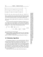
N = 1
2
3
4
(total after N = 4)
Figure 4.2.1. Sequential calls to the routine trapzd incorporate the information from previous calls and
evaluate the integrand only at those new points necessary to refine the grid. The bottom line shows the
totality of function evaluations after the fourth call. The routine qsimp, by weighting the intermediate
results, transforms the trapezoid rule into Simpson’s rule with essentially no additional overhead.
There are also formulas of higher order for this situation, but we will refrain from
giving them.
The semi-open formulas arejusttheobviouscombinations ofequations(4.1.11)–
(4.1.14) with (4.1.15)–(4.1.18), respectively. At the closed end of the integration,
use the weights from the former equations; at the open end use the weights from
the latter equations. One example should give the idea, the formula with error term
decreasing as 1/N
3
whichisclosedontherightandopenontheleft:

x
N
x
1
f(x)dx = h


23
12
f
2
+
7
12
f
3
+ f
4
+ f
5
+
···+f
N−2
+
13
12
f
N −1
+
5
12
f
N

+ O


1
N
3

(4.1.20)
CITED REFERENCES AND FURTHER READING:
Abramowitz, M., and Stegun, I.A. 1964,
Handbook of Mathematical Functions
, Applied Mathe-
matics Series, Volume 55 (Washington: National Bureau of Standards; reprinted 1968 by
Dover Publications, New York),
§
25.4. [1]
Isaacson, E., and Keller, H.B. 1966,
Analysis of Numerical Methods
(New York: Wiley),
§
7.1.
4.2 Elementary Algorithms
Our starting point is equation (4.1.11), the extended trapezoidal rule. There are
two facts about the trapezoidal rule which make it the starting point for a variety of
algorithms. One fact is rather obvious, while the second is rather “deep.”
The obvious fact is that, for a fixed function f(x) to be integrated between fixed
limits a and b, one can double the number of intervals in the extended trapezoidal
rule without losing the benefit of previous work. The coarsest implementation of
the trapezoidal rule is to average the function at its endpoints a and b.Thefirst
stage of refinement is to add to this average the value of the function at the halfway
point. The second stage of refinement is to add the values at the 1/4 and 3/4 points.
Andsoon(seeFigure4.2.1).
Without further ado we can write a routine with this kind of logic to it:

4.2 Elementary Algorithms
137
Sample page from NUMERICAL RECIPES IN C: THE ART OF SCIENTIFIC COMPUTING (ISBN 0-521-43108-5)
Copyright (C) 1988-1992 by Cambridge University Press.Programs Copyright (C) 1988-1992 by Numerical Recipes Software.
Permission is granted for internet users to make one paper copy for their own personal use. Further reproduction, or any copying of machine-
readable files (including this one) to any servercomputer, is strictly prohibited. To order Numerical Recipes books,diskettes, or CDROMs
visit website or call 1-800-872-7423 (North America only),or send email to (outside North America).
#define FUNC(x) ((*func)(x))
float trapzd(float (*func)(float), float a, float b, int n)
This routine computes the
n
th stage of refinement of an extended trapezoidal rule.
func
is input
as a pointer to the function to be integrated between limits
a
and
b
, also input. When called with
n
=1, the routine returns the crudest estimate of

b
a
f(x)dx. Subsequent calls with
n
=2,3,...
(in that sequential order) will improve the accuracy by adding 2
n-2
additional interior points.

{
float x,tnm,sum,del;
static float s;
int it,j;
if (n == 1) {
return (s=0.5*(b-a)*(FUNC(a)+FUNC(b)));
} else {
for (it=1,j=1;j<n-1;j++) it <<= 1;
tnm=it;
del=(b-a)/tnm; This is the spacing of the points to be added.
x=a+0.5*del;
for (sum=0.0,j=1;j<=it;j++,x+=del) sum += FUNC(x);
s=0.5*(s+(b-a)*sum/tnm); This replaces s by its refined value.
return s;
}
}
The above routine (trapzd) is a workhorse that can be harnessed in several
ways. The simplest and crudest is to integrate a functionby the extended trapezoidal
rule where you know in advance (we can’t imagine how!) the number of steps you
want. If you want 2
M
+1, you can accomplish this by the fragment
for(j=1;j<=m+1;j++) s=trapzd(func,a,b,j);
with the answer returned as s.
Much better, of course, is to refine the trapezoidal rule until some specified
degree of accuracy has been achieved:
#include <math.h>
#define EPS 1.0e-5
#define JMAX 20
float qtrap(float (*func)(float), float a, float b)

Returns the integral of the function
func
from
a
to
b
. The parameters
EPS
can be set to the
desired fractional accuracy and
JMAX
sothat2tothepower
JMAX-1
is the maximum allowed
number of steps. Integration is performed by the trapezoidal rule.
{
float trapzd(float (*func)(float), float a, float b, int n);
void nrerror(char error_text[]);
int j;
float s,olds;
olds = -1.0e30; Any number that is unlikely to be the average of the
function at its endpoints will do here.for (j=1;j<=JMAX;j++) {
s=trapzd(func,a,b,j);
if (j > 5) Avoid spurious early convergence.
if (fabs(s-olds) < EPS*fabs(olds) ||
(s == 0.0 && olds == 0.0)) return s;
olds=s;
}
nrerror("Too many steps in routine qtrap");
return 0.0; Never get here.

}
138
Chapter 4. Integration of Functions
Sample page from NUMERICAL RECIPES IN C: THE ART OF SCIENTIFIC COMPUTING (ISBN 0-521-43108-5)
Copyright (C) 1988-1992 by Cambridge University Press.Programs Copyright (C) 1988-1992 by Numerical Recipes Software.
Permission is granted for internet users to make one paper copy for their own personal use. Further reproduction, or any copying of machine-
readable files (including this one) to any servercomputer, is strictly prohibited. To order Numerical Recipes books,diskettes, or CDROMs
visit website or call 1-800-872-7423 (North America only),or send email to (outside North America).
Unsophisticated as it is, routine qtrap is in fact a fairly robust way of doing
integrals of functions that are not very smooth. Increased sophistication will usually
translate into a higher-order method whose efficiency will be greater only for
sufficiently smooth integrands. qtrap is the method of choice, e.g., for an integrand
which is a function of a variable that is linearly interpolated between measured data
points. Be sure that you do not require too stringent an EPS, however: If qtraptakes
too many steps in trying to achieve your required accuracy, accumulated roundoff
errors may start increasing, and the routine may never converge. A value 10
−6
is just on the edge of trouble for most 32-bit machines; it is achievable when the
convergence is moderately rapid, but not otherwise.
We come now to the “deep” fact about the extended trapezoidal rule, equation
(4.1.11). It is this: The error of the approximation, which begins with a term of
order 1/N
2
, is in fact entirely even when expressed in powers of 1/N. This follows
directly from the Euler-Maclaurin Summation Formula,

x
N
x
1

f(x)dx = h

1
2
f
1
+ f
2
+ f
3
+ ···+f
N−1
+
1
2
f
N

−
B
2
h
2
2!
(f

N
− f

1

) −···−
B
2k
h
2k
(2k)!
(f
(2k−1)
N
− f
(2k−1)
1
) −···
(4.2.1)
Here B
2k
is a Bernoulli number, defined by the generating function
t
e
t
− 1
=
∞

n=0
B
n
t
n
n!

(4.2.2)
with the first few even values (odd values vanish except for B
1
= −1/2)
B
0
=1 B
2
=
1
6
B
4
=−
1
30
B
6
=
1
42
B
8
= −
1
30
B
10
=
5

66
B
12
= −
691
2730
(4.2.3)
Equation (4.2.1) is not a convergent expansion, but rather only an asymptotic
expansion whose error when truncated at any point is always less than twice the
magnitude of the first neglected term. The reason that it is not convergent is that
the Bernoulli numbers become very large, e.g.,
B
50
=
495057205241079648212477525
66
The key point is that only even powers of h occur in the error series of (4.2.1).
This fact is not, in general, shared by the higher-order quadrature rules in §4.1.
For example, equation (4.1.12) has an error series beginning with O(1/N
3
), but
continuing with all subsequent powers of N: 1/N
4
, 1/N
5
,etc.
Suppose we evaluate (4.1.11) with N steps, getting a result S
N
, and then again
with 2N steps, getting a result S

2N
. (This is done by any two consecutive calls of
4.2 Elementary Algorithms
139
Sample page from NUMERICAL RECIPES IN C: THE ART OF SCIENTIFIC COMPUTING (ISBN 0-521-43108-5)
Copyright (C) 1988-1992 by Cambridge University Press.Programs Copyright (C) 1988-1992 by Numerical Recipes Software.
Permission is granted for internet users to make one paper copy for their own personal use. Further reproduction, or any copying of machine-
readable files (including this one) to any servercomputer, is strictly prohibited. To order Numerical Recipes books,diskettes, or CDROMs
visit website or call 1-800-872-7423 (North America only),or send email to (outside North America).
trapzd.) The leading error term in the second evaluation will be 1/4 the size of the
error in the first evaluation. Therefore the combination
S =
4
3
S
2N
−
1
3
S
N
(4.2.4)
will cancel out the leading order error term. But there is no error term of order
1/N
3
, by (4.2.1). The surviving error is of order 1/N
4
, the same as Simpson’s rule.
In fact, it should not take long for you to see that (4.2.4) is exactly Simpson’s rule
(4.1.13), alternating 2/3’s, 4/3’s, and all. This is the preferred method for evaluating

that rule, and we can write it as a routine exactly analogous to qtrap above:
#include <math.h>
#define EPS 1.0e-6
#define JMAX 20
float qsimp(float (*func)(float), float a, float b)
Returns the integral of the function
func
from
a
to
b
. The parameters
EPS
can be set to the
desired fractional accuracy and
JMAX
sothat2tothepower
JMAX-1
is the maximum allowed
number of steps. Integration is performed by Simpson’s rule.
{
float trapzd(float (*func)(float), float a, float b, int n);
void nrerror(char error_text[]);
int j;
float s,st,ost,os;
ost = os = -1.0e30;
for (j=1;j<=JMAX;j++) {
st=trapzd(func,a,b,j);
s=(4.0*st-ost)/3.0; Compare equation (4.2.4), above.
if (j > 5) Avoid spurious early convergence.

if (fabs(s-os) < EPS*fabs(os) ||
(s == 0.0 && os == 0.0)) return s;
os=s;
ost=st;
}
nrerror("Too many steps in routine qsimp");
return 0.0; Never get here.
}
The routine qsimp will in general be more efficient than qtrap (i.e., require
fewer function evaluations) when the function to be integrated has a finite 4th
derivative (i.e., a continuous 3rd derivative). The combination of qsimp and its
necessary workhorse trapzd is a good one for light-duty work.
CITED REFERENCES AND FURTHER READING:
Stoer, J., and Bulirsch, R. 1980,
Introduction to Numerical Analysis
(New York: Springer-Verlag),
§
3.3.
Dahlquist, G., and Bjorck, A. 1974,
Numerical Methods
(Englewood Cliffs, NJ: Prentice-Hall),
§§
7.4.1–7.4.2.
Forsythe, G.E., Malcolm, M.A., and Moler, C.B. 1977,
Computer Methods for Mathematical
Computations
(Englewood Cliffs, NJ: Prentice-Hall),
§
5.3.
140

Chapter 4. Integration of Functions
Sample page from NUMERICAL RECIPES IN C: THE ART OF SCIENTIFIC COMPUTING (ISBN 0-521-43108-5)
Copyright (C) 1988-1992 by Cambridge University Press.Programs Copyright (C) 1988-1992 by Numerical Recipes Software.
Permission is granted for internet users to make one paper copy for their own personal use. Further reproduction, or any copying of machine-
readable files (including this one) to any servercomputer, is strictly prohibited. To order Numerical Recipes books,diskettes, or CDROMs
visit website or call 1-800-872-7423 (North America only),or send email to (outside North America).
4.3 Romberg Integration
We can view Romberg’s method as the natural generalization of the routine
qsimp in the last section to integration schemes that are of higher order than
Simpson’s rule. The basic idea is to use the results from k successive refinements
of the extended trapezoidal rule (implemented in trapzd) to remove all terms in
the error series up to but not including O(1/N
2k
). The routine qsimp is the case
of k =2. This is one example of a very general idea that goes by the name of
Richardson’s deferred approach to the limit: Perform some numerical algorithm for
various values of a parameter h, and then extrapolate the result to the continuum
limit h =0.
Equation (4.2.4), which subtracts off the leading error term, is a special case of
polynomial extrapolation. In the more general Romberg case, we can use Neville’s
algorithm (see §3.1) to extrapolate the successive refinements to zero stepsize.
Neville’s algorithmcan in fact be coded veryconcisely withina Romberg integration
routine. For clarity of the program, however, it seems better to do the extrapolation
by function call to polint, already given in §3.1.
#include <math.h>
#define EPS 1.0e-6
#define JMAX 20
#define JMAXP (JMAX+1)
#define K 5
Here

EPS
is the fractional accuracy desired, as determined by the extrapolation error estimate;
JMAX
limits the total number of steps;
K
is the number of points used in the extrapolation.
float qromb(float (*func)(float), float a, float b)
Returns the integral of the function
func
from
a
to
b
. Integration is performed by Romberg’s
method of order 2
K
, where, e.g.,
K
=2 is Simpson’s rule.
{
void polint(float xa[], float ya[], int n, float x, float *y, float *dy);
float trapzd(float (*func)(float), float a, float b, int n);
void nrerror(char error_text[]);
float ss,dss;
float s[JMAXP],h[JMAXP+1]; These store the successive trapezoidal approxi-
mations and their relative stepsizes.int j;
h[1]=1.0;
for (j=1;j<=JMAX;j++) {
s[j]=trapzd(func,a,b,j);
if (j >= K) {

polint(&h[j-K],&s[j-K],K,0.0,&ss,&dss);
if (fabs(dss) <= EPS*fabs(ss)) return ss;
}
h[j+1]=0.25*h[j];
This is a key step: The factor is 0.25 even though the stepsize is decreased by only
0.5. This makes the extrapolation a polynomial in h
2
as allowed by equation (4.2.1),
not just a polynomial in h.
}
nrerror("Too many steps in routine qromb");
return 0.0; Never get here.
}
The routine qromb, along with its required trapzd and polint, is quite
powerful for sufficiently smooth (e.g., analytic) integrands, integrated over intervals