Tài liệu Integration of Functions part 4 docx

140
Chapter 4. Integration of Functions
Sample page from NUMERICAL RECIPES IN C: THE ART OF SCIENTIFIC COMPUTING (ISBN 0-521-43108-5)
Copyright (C) 1988-1992 by Cambridge University Press.Programs Copyright (C) 1988-1992 by Numerical Recipes Software.
Permission is granted for internet users to make one paper copy for their own personal use. Further reproduction, or any copying of machine-
readable files (including this one) to any servercomputer, is strictly prohibited. To order Numerical Recipes books,diskettes, or CDROMs
visit website or call 1-800-872-7423 (North America only),or send email to (outside North America).
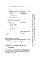
4.3 Romberg Integration
We can view Romberg’s method as the natural generalization of the routine
qsimp in the last section to integration schemes that are of higher order than
Simpson’s rule. The basic idea is to use the results from k successive refinements
of the extended trapezoidal rule (implemented in trapzd) to remove all terms in
the error series up to but not including O(1/N
2k
). The routine qsimp is the case
of k =2. This is one example of a very general idea that goes by the name of
Richardson’s deferred approach to the limit: Perform some numerical algorithm for
various values of a parameter h, and then extrapolate the result to the continuum
limit h =0.
Equation (4.2.4), which subtracts off the leading error term, is a special case of
polynomial extrapolation. In the more general Romberg case, we can use Neville’s
algorithm (see §3.1) to extrapolate the successive refinements to zero stepsize.
Neville’s algorithmcan in fact be coded very concisely withina Romberg integration
routine. For clarity of the program, however, it seems better to do the extrapolation
by function call to polint, already given in §3.1.
#include <math.h>
#define EPS 1.0e-6
#define JMAX 20
#define JMAXP (JMAX+1)
#define K 5
Here

EPS
is the fractional accuracy desired, as determined by the extrapolation error estimate;
JMAX
limits the total number of steps;
K
is the number of points used in the extrapolation.
float qromb(float (*func)(float), float a, float b)
Returns the integral of the function
func
from
a
to
b
. Integration is performed by Romberg’s
method of order 2
K
, where, e.g.,
K
=2 is Simpson’s rule.
{
void polint(float xa[], float ya[], int n, float x, float *y, float *dy);
float trapzd(float (*func)(float), float a, float b, int n);
void nrerror(char error_text[]);
float ss,dss;
float s[JMAXP],h[JMAXP+1]; These store the successive trapezoidal approxi-
mations and their relative stepsizes.int j;
h[1]=1.0;
for (j=1;j<=JMAX;j++) {
s[j]=trapzd(func,a,b,j);
if (j >= K) {

polint(&h[j-K],&s[j-K],K,0.0,&ss,&dss);
if (fabs(dss) <= EPS*fabs(ss)) return ss;
}
h[j+1]=0.25*h[j];
This is a key step: The factor is 0.25 even though the stepsize is decreased by only
0.5. This makes the extrapolation a polynomial in h
2
as allowed by equation (4.2.1),
not just a polynomial in h.
}
nrerror("Too many steps in routine qromb");
return 0.0; Never get here.
}
The routine qromb, along with its required trapzd and polint, is quite
powerful for sufficiently smooth (e.g., analytic) integrands, integrated over intervals
4.4 Improper Integrals
141
Sample page from NUMERICAL RECIPES IN C: THE ART OF SCIENTIFIC COMPUTING (ISBN 0-521-43108-5)
Copyright (C) 1988-1992 by Cambridge University Press.Programs Copyright (C) 1988-1992 by Numerical Recipes Software.
Permission is granted for internet users to make one paper copy for their own personal use. Further reproduction, or any copying of machine-
readable files (including this one) to any servercomputer, is strictly prohibited. To order Numerical Recipes books,diskettes, or CDROMs
visit website or call 1-800-872-7423 (North America only),or send email to (outside North America).
which contain no singularities, and where the endpointsare also nonsingular. qromb,
in such circumstances, takes many, many fewer function evaluations than either of
the routines in §4.2. For example, the integral

2
0
x
4

log(x +

x
2
+1)dx
converges (with parameters as shown above) on the very first extrapolation, after
just 5 calls to trapzd, while qsimp requires 8 calls (8 times as many evaluations of
the integrand) and qtrap requires 13 calls (making 256 times as many evaluations
of the integrand).
CITED REFERENCES AND FURTHER READING:
Stoer, J., and Bulirsch, R. 1980,
Introduction to Numerical Analysis
(New York: Springer-Verlag),
§§
3.4–3.5.
Dahlquist, G., and Bjorck, A. 1974,
Numerical Methods
(Englewood Cliffs, NJ: Prentice-Hall),
§§
7.4.1–7.4.2.
Ralston, A., and Rabinowitz, P. 1978,
A First Course in Numerical Analysis
, 2nd ed. (New York:
McGraw-Hill),
§
4.10–2.
4.4 Improper Integrals
For our present purposes, an integral will be “improper” if it has any of the
following problems:
• its integrand goes to a finite limitingvalue at finite upper and lower limits,

but cannot be evaluated right on one of thoselimits(e.g., sin x/x at x =0)
• its upper limit is ∞ , or its lower limit is −∞
• it has an integrable singularity at either limit (e.g., x
−1/2
at x =0)
• it has an integrable singularity at a known place between its upper and
lower limits
• it has an integrable singularity at an unknown place between its upper
and lower limits
If an integral is infinite (e.g.,

∞
1
x
−1
dx), or does not exist in a limiting sense
(e.g.,

∞
−∞
cos xdx), we do not call it improper; we call it impossible. No amount of
clever algorithmics will return a meaningful answer to an ill-posed problem.
In this section we will generalize the techniques of the preceding two sections
to cover the first four problems on the above list. A more advanced discussion of
quadrature with integrable singularities occurs in Chapter 18, notably §18.3. The
fifth problem, singularity at unknown location, can really only be handled by the
use of a variable stepsize differential equation integration routine, as will be given
in Chapter 16.
We need a workhorse like the extended trapezoidal rule (equation 4.1.11), but
one which is an open formula in the sense of §4.1, i.e., does not require the integrand

to be evaluated at the endpoints. Equation (4.1.19), the extended midpoint rule, is
the best choice. The reason is that (4.1.19) shares with (4.1.11) the “deep” property