Tài liệu Laser điốt được phân phối thông tin phản hồi và các bộ lọc du dương quang P3 docx

3
Structural Impacts on the Solutions
of Coupled Wave Equations:
An Overview
3.1 INTRODUCTION
The introduction of semiconductor lasers has boosted the development of coherent optical
communication systems. With the built-in wavelength selection mechanism, distributed
feedback semiconductor laser diodes with a higher gain margin are superior to the Fabry–
Perot laser in that a single longitudinal mode of lasing can be achieved.
In this chapter, results obtained from the threshold analysis of conventional and single-
phase-shifted DFB lasers will be investigated. In particular, structural impacts on the
threshold characteristic will be discussed in a systematic way. The next two sections of this
chapter present solutions of the coupled wave equations in DFB laser diode structures. In
section 3.4 the concepts of mode discrimination and gain margin are discussed. The
threshold analysis of a conventional DFB laser diode is studied in section 3.5, whilst the
impact of corrugation phase at the DFB laser diode facets is discussed in section 3.6. By
introducing a phase shift along the corrugations of DFB LDs, the degenerate oscillating
characteristic of the conventional DFB LD can be removed. In section 3.7, structural
impacts due to the phase shift and the corresponding phase shift position (PSP) will be
considered.
As mentioned earlier in Chapter 2, the introduction of the coupling coefficient  into the
coupled wave equations plays a vital role since it measures the strength of feedback provided
by the corrugation. In section 3.7, the effect of the selection of corrugation shape on the
magnitude of  will be presented. With a =2 phase shift fabricated at the centre of the DFB
cavity, the quarterly-wavelength-shifted (QWS) DFB LD oscillates at the Bragg wavelength.
However, the deterioration of gain margin limits its use as the current injection increases.
This phenomenon induced by the spatial hole burning effect, which is the major drawback of
the QWS laser structure, will be examined at the end of this chapter. The limited
application of the eigenvalue equation in solving the coupled wave equations will also be
considered.
Distributed Feedback Laser Diodes and Optical Tunable Filters H. Ghafouri–Shiraz

# 2003 John Wiley & Sons, Ltd ISBN: 0-470-85618-1
3.2 SOLUTIONS OF THE COUPLED WAVE EQUATIONS
In Chapter 2 it was shown that the characteristics of DFB LDs can be described by a pair of
coupled wave equations. The strength of the feedback induced by the perturbed refractive
index or gain is measured by the coupling coefficient. Relationships between the forward
and the backward coupling coefficients 
RS
and 
SR
were derived for purely index-coupled,
mixed-coupled and purely gain-coupled structures. By assuming a zero phase difference
between the index and the gain term, the complex coupling coefficient could be expressed as

RS
¼ 
SR
¼ 
i
þ j
g
¼  ð3:1Þ
where  becomes a complex coupling coefficient. According to eqn (2.98), the trial solution
of the coupled wave equation can be expressed in terms of the Bragg propagation constant
such that
EðzÞ¼RðzÞe
Àjb
0
z
þ SðzÞe
jb

0
z
ð3:2Þ
where the coefficients RðzÞ and SðzÞ are given as [1]
RðzÞ¼R
1
e
ðgzÞ
þ R
2
e
ðÀgzÞ
ð3:3aÞ
and
SðzÞ¼S
1
e
ðgzÞ
þ S
2
e
ðÀgzÞ
ð3:3bÞ
In the above equations, R
1
, R
2
, S
1
and S

2
are complex coefficients and g is the complex
propagation constant to be determined from the boundary conditions at the laser facets.
Without loss of generality, one can assume ReðgÞ > 0. As a result, those terms with
coefficients R
1
and S
2
become amplified as the waves propagate along the cavity. By
contrast, those terms with coefficients R
2
and S
1
are attenuated. By combining the above
equations with eqn (3.2), it can be shown easily that the propagation constant of the
amplified waves becomes b
0
À ImðgÞ whilst the decaying waves propagate at b
0
þ ImðgÞ.
By substituting eqns (3.3a) and (3.3b) into the coupled wave equations, the following
relations are obtained by collecting identical exponential terms [2]
^
 R
1
¼ je
Àj
S
1
ð3:4aÞ

 R
2
¼ je
Àj
S
2
ð3:4bÞ
 S
1
¼ je
j
R
1
ð3:4cÞ
^
 S
2
¼ je
j
R
2
ð3:4dÞ
where
^
 ¼ 
s
À jd À g ð3:5aÞ
 ¼ 
s
À jd þ g ð3:5bÞ

By comparing eqns (3.4a) and (3.4c), a non-trivial solution exists if the following equation is
satisfied
 ¼
^

j
¼
j

ð3:6Þ
80
STRUCTURAL IMPACTS ON THE SOLUTIONS OF COUPLED WAVE EQUATIONS
Based on the equation shown above, eqn (3.4) is simplified to become
R
1
¼
1

e
Àj
S
1
ð3:7aÞ
R
2
¼ e
Àj
S
2
ð3:7bÞ

Similarly, by equating eqns (3.4a) and (3.4c), one obtains
g
2
¼ð
s
À j dÞ
2
þ 
2
ð3:8Þ
It is important that the dispersion equation shown above is independent of the residue
corrugation phase .
With a finite laser cavity length L extending from z ¼ z
1
to z ¼ z
2
(where both z
1
and z
2
are assumed to be greater than zero), the boundary conditions at the terminating facets
become
Rðz
1
Þ e
Àj b
0
z
1
¼

^
r
1
Sðz
1
Þ e
j b
0
z
1
ð3:9aÞ
Sðz
2
Þ e
j b
0
z
2
¼
^
r
2
Rðz
2
Þ e
Àj b
0
z
2
ð3:9bÞ

where
^
r
1
and
^
r
2
are amplitude reflection coefficients at the laser facets z
1
and z
2
, respectively.
According to eqns (3.3) and (3.4), the above equations could be expanded in such a way that
R
2
¼
ð1 À  r
1
Þ e
2g z
1
r
1
= À 1
Á R
1
ð3:10aÞ
R
2

¼
ðr
2
À  Þ e
2g z
2
1= À r
2
Á R
1
ð3:10bÞ
In the above equation, all RðzÞ and SðzÞ terms are expressed in terms of R
1
and R
2
, whilst r
1
and r
2
are the complex field reflectivities of the left and the right facets, respectively such that
r
1
¼
^
r
1
e
2jb
0
z

1
e
j
¼
^
r
1
e
j 
1
ð3:11aÞ
r
2
¼
^
r
2
e
À2jb
0
z
2
e
Àj
¼
^
r
2
e
j 

2
ð3:11bÞ
with
1
and
2
being the corresponding corrugation phases at the facets. Equations (3.10a)
and (3.10b) are homogeneous in R
1
and R
2
. In order to have non-trivial solutions, the
following condition must be satisfied
ð1 À  r
1
Þ e
2g z
1
r
1
À 
¼
ðr
2
À Þ e
2gz
2
1 À  r
2
ð3:12Þ

Then the above equation can be solved for  and 1= whilst employing the relation
g ¼
Àj
2
 À
1


ð3:13Þ
SOLUTIONS OF THE COUPLED WAVE EQUATIONS
81
derived from eqns (3.5a) and (3.5b). After some lengthy manipulation [2], one ends up with
an eigenvalue equation
gL ¼
Àj sinhðLÞ
D
Á r
1
þ r
2
ðÞ1 À r
1
r
2
ðÞcoshðgLÞÆ 1 þ r
1
r
2
ðÞÁ
1

2
no
ð3:14Þ
where
Á ¼ðr
1
À r
2
Þ
2
sinh
2
ðgLÞþð1 À r
1
r
2
Þ
2
ð3:15aÞ
D ¼ð1 þ r
1
r
2
Þ
2
À 4 r
1
r
2
cosh

2
ðg LÞð3:15bÞ
r
1
¼
^
r
1
e
2jb
0
z
1
e
j
¼
^
r
1
e
j
1
ð3:15cÞ
r
2
¼
^
r
2
e

À2jb
0
z
2
e
Àj
¼
^
r
2
e
j
2
ð3:15dÞ
By squaring eqn (3.1), and after some simplification, one ends up with a transcendental
function
ðgLÞ
2
þðLÞ
2
sinh
2
ðgLÞð1 À r
2
1
Þð1 À r
2
2
Þ
þ 2j L ðr

1
þ r
2
Þ
2
ð1 À r
1
r
2
Þ gL sinhðgLÞ coshðgLÞ¼0 ð3:16Þ
In the above equation, there are four parameters which govern the threshold characteristics
of DFB laser structures. These are the coupling coefficient , the laser cavity length L and
the complex facet reflectivities r
1
and r
2
. Due to the complex nature of the above equation,
numerical methods like the Newton–Raphson iteration technique can be used, provided that
the Cauchy–Riemann condition on complex analytical functions is satisfied.
Before starting the Newton–Raphson iteration, an initial value of ð; Þ
ini
is chosen from a
selected range of ð; Þ values. Usually, the first selected guess will not be a solution of the
threshold equation and hence the iteration continues. At the end of the first iteration, a new
pair of ð
0
;
0
Þ will be generated and checked to see if it satisfies the threshold equation. The
iteration will continue until the newly generated ð

0
;
0
Þ pair satisfies the threshold equation
within a reasonable range of error. Starting with different initial guesses of ð; Þ
ini
, other
oscillating modes can be determined in a similar way. By collecting all ð
0
;
0
Þ pairs that
satisfy the threshold equation, the one showing the smallest amplitude gain will then become
the lasing mode. The final value ð; Þ
final
is then stored up for later use, in which the
threshold current and the lasing wavelength of the LD are to be decided. In general,
eqn (3.16) characterises all conventional DFB semiconductor LDs with continuous
corrugations fabricated along the laser cavity.
3.3 SOLUTIONS OF COMPLEX TRANSCENDENTAL EQUATIONS
USING THE NEWTON–RAPHSON APPROXIMATION
All complex transcendental equations can be expressed in a general form such that
WðzÞ¼UðzÞþj VðzÞ¼0 ð3:17Þ
82
STRUCTURAL IMPACTS ON THE SOLUTIONS OF COUPLED WAVE EQUATIONS
where z ¼ x þ j y is a complex number and UðzÞ and VðzÞ are, respectively, the real and
imaginary parts of the complex function. From the above equation, one can deduce the
following equality easily
UðzÞ¼VðzÞ¼0 ð3:18Þ
By taking the first-order derivative of eqn (3.17) with respect to z, one can obtain

@W
@z
¼
@U
@z
þ j
@V
@z
¼
@U
@x
þ j
@V
@x
ð3:19Þ
The second equality sign can be obtained using the chain rule. Applying the Taylor series,
the functions U(z) and V(z) can be approximated about the exact solution ðx
req
, y
req
Þ such
that
Uðx
req
; y
req
Þ¼Ux; yðÞþ
@U
@x
ðx

req
À xÞþ
@U
@y
ðy
req
À yÞð3:20Þ
Vðx
req
; y
req
Þ¼Vx; yðÞþ
@V
@x
ðx
req
À xÞþ
@V
@y
ðy
req
À yÞð3:21Þ
where the values of (x, y) chosen are sufficiently close to the exact solutions. Other higher
derivative terms from the Taylor series have been ignored. One then obtains the following
equations for x
req
and y
req
from the above simultaneous equations [2]
x

req
¼ x þ
Vðx; yÞ
@U
@y
À Uðx; yÞ
@V
@y
Det
ð3:22Þ
y
req
¼ y þ
Uðx; yÞ
@V
@x
À Vðx; yÞ
@U
@x
Det
ð3:23Þ
where
Det ¼
@U
@x

2
þ
@V
@y


2
ð3:24Þ
Terms like @U=@x, @V=@x, @U=@y and @V=@y are the first derivatives of functions U(z) and
V(z).
For an analytical complex function W(z), the Cauchy–Riemann condition which states
that
@U
@x
¼
@V
@y
;
@U
@y
¼À
@V
@x
ð3:25Þ
must be satisfied [3].
SOLUTIONS OF COMPLEX TRANSCENDENTAL EQUATIONS
83
On replacing all the @=@y terms with @=@x using the above Cauchy–Riemann condition,
eqns (3.22) and (3.24) can be simplified such that
Det ¼ 2
@U
@x

2
ð3:26Þ

x
req
¼ x À
Vðx; yÞ
@V
@x
þ Uðx; yÞ
@U
@x
Det
ð3:27Þ
Here, only the first-order derivative terms @U=@x and @V=@x are used. These can be
determined from the complex function of eqn (3.19).
Given an initial guess of ðx; yÞ, the numerical iteration process then starts. A new guess is
generated by following eqns (3.23), (3.26) and (3.27). Unless the new guess is sufficiently
close to the exact solution (within 10
À9
, let’s say), the new guess solution formed will
become the initial guess of the next iteration. The iteration process continues until
approximate solutions of ðx
req
, y
req
Þ appear.
The advantages of this method are its speed and flexibility. In addition, the derivative term
@W=@z is found analytically first, before any numerical iteration is started. Using this
method, one can avoid any errors associated with other numerical methods such as
numerical differentiation.
3.4 CONCEPTS OF MODE DISCRIMINATION
AND GAIN MARGIN

At a fixed value of , pairs of ð; Þ
final
can be determined following the method discussed in
the previous section. Each ð; Þ
final
pair, which represents an oscillation mode, is plotted on
the – plane. Similarly, pairs of ð; Þ
final
values can be obtained by changing the values of
. By plotting all ð; Þ
final
points on the – plane, the mode spectrum of the DFB LD is
formed. A simplified – plot is shown in Fig. 3.1. Different symbols shown represent
various longitudinal modes obtained for various coupling coefficients whilst the solid curve
shows how longitudinal modes join to form an oscillating mode.
When the biasing current increases, the longitudinal mode showing the smallest amplitude
gain will reach the threshold condition first and begin to lase. Other modes failing to reach
the threshold condition will then be suppressed and become non-lasing side modes. The –
plane is split into two halves by the  ¼ 0 line, or the Bragg wavelength. As one moves
along the positive -axis, any oscillation modes encountered will be denoted as the þ1, þ2
modes and so on. Similarly, negative values such as À1, À2 are used for the modes found on
the negative -axis.
The importance of the single longitudinal mode (SLM) in coherent optical communica-
tions has been discussed earlier in Chapter 1. To measure the stability of the lasing spectrum,
one needs to determine the amplitude gain difference between the lasing mode and the most
probable side mode of the DFB laser ½4; 5. A larger amplitude gain difference, better known
as the gain margin ðÁÞ, implies a better mode discrimination. In other words, the SLM
oscillation in the DFB LD involved is said to be more stable. In practice, the actual
requirement of Á may vary from one system to another depending on the encoding format
84

STRUCTURAL IMPACTS ON THE SOLUTIONS OF COUPLED WAVE EQUATIONS
(return to zero, RZ, or non-return to zero, NRZ), transmission rate, the biasing condition of
the laser sources, the length and characteristics of the single-mode fibre (SMF) used. A
simulation based on a 20 km dispersive SMF [6] indicated that a Á of 5 cm
À1
is required
for a 2.4 Gb s
À1
data transmission in order that a bit error rate, BER < 10
À9
can be achieved.
A detailed analysis of the requirement of Á under different system configurations is clearly
beyond the scope of the present analysis. On the other hand, from the above data one can get
some idea of the typical values of gain margin required in a coherent optical communication
system.
The value of the gain margin, however, is difficult to measure directly from an experiment.
An alternative method is to measure the spontaneous emission spectrum. For a stable SLM
source, a minimum side mode suppression ratio (SMSR) of 25 dB [7] between the power of
the lasing mode and the most probable side mode is necessary.
3.5 THRESHOLD ANALYSIS OF A CONVENTIONAL DFB LASER
For a conventional DFB laser having zero facet reflection, the threshold equation (3.16)
becomes
j g L ¼ÆL sinhðLÞð3:28Þ
Using the Newton–Raphson iteration approach, the eigenvalue equation can be solved as a
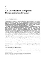
fixed coupling coefficient. Results obtained for the above equation are shown in Fig. 3.2. All
Figure 3.1 A simplified – plot showing the mode spectrum and the oscillating mode of a DFB LD.
Different symbols are used to show longitudinal modes obtained from various  values.
THRESHOLD ANALYSIS OF A CONVENTIONAL DFB LASER
85
parameters used have been normalised with respect to the overall cavity length L. Discrete

values of L have been selected between 0.25 and 10.0. As shown in the inset of Fig. 3.2,
solutions obtained from various L products are shown using different symbols. Oscillation
modes are then formed by joining the appropriate solutions together. Solid lines have been
used to represent the À4toþ4 modes. From the figure, it is clear that oscillating modes
distribute symmetrically with respect to the Bragg wavelength, whilst no oscillation is found
at the Bragg wavelength. Furthermore, it can be seen that the þ1 and À1 modes although
having different lasing wavelengths share the same amplitude gain. As a result, degenerate
oscillation occurs and these modes will have the same chance to lase once the lasing
condition is reached. Figure 3.2 also reveals that the amplitude of the threshold gain
decreases with increasing values of L. Since a larger value of  implies a stronger optical
feedback, a smaller threshold gain results. Similarly, lasers having a long cavity length help
to reduce the amplitude gain since a larger single pass gain can be achieved.
With no oscillation found at the Bragg wavelength, a stop band region is formed between
the þ1 and À1 modes of the conventional mirrorless DFB LD. From Fig. 3.2, one can
conclude that the normalised stop band width is a function of L. Although the change in
stop band width becomes less noticeable at lower values of L, the measurement of the stop
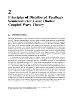
band width has been used to determine the coupling coefficient of DFB LDs [8]. Figure 3.3
shows the characteristic of a DFB LD having finite facet reflections. It is shown in the figure
that the mode distribution is no longer symmetrical and no oscillation is found at the
Bragg wavelength. The À1 mode, having the smallest amplitude gain, becomes the lasing
mode.
Figure 3.2 Relationship between the amplitude threshold gain and the detuning coefficient of a
mirrorless index-coupled DFB LD.
86
STRUCTURAL IMPACTS ON THE SOLUTIONS OF COUPLED WAVE EQUATIONS