Tài liệu Laser điốt được phân phối thông tin phản hồi và các bộ lọc du dương quang P4 ppt

4
Transfer Matrix Modelling in
DFB Semiconductor Lasers
4.1 INTRODUCTION
In Chapter 3, eigenvalue equations were derived by matching boundary conditions inside
DFB laser cavities. From the eigenvalue problem, the lasing threshold characteristic of DFB
lasers is determined. The single /2-phase-shifted (PS) DFB laser is fabricated with a phase
discontinuity of /2 at or near the centre of the laser cavity. It is characterised by Bragg
oscillation and a high gain margin value. On the other hand, the SLM deteriorates quickly
when the optical power of the laser diode increases. This phenomenon, known as spatial hole
burning, limits the maximum single-mode optical power and consequently the spectral
linewidth. Using a multiple-phase-shift (MPS) DFB laser structure, the electric field
distribution is flattened and hence the spatial hole burning is suppressed.
In dealing with such a complicated DFB laser structure, it is tedious to match all the
boundary conditions. A more flexible method which is capable of handling different types of
DFB laser structures is necessary. In section 4.2, the transfer matrix method (TMM) [1– 4]
will be introduced and explored comprehensively. From the coupled wave equations, it is
found that the field propagation inside a corrugated waveguide (e.g. the DFB laser cavity)
can be represented by a transfer matrix. Provided that the electric fields at the input plane are
known, the matrix acts as a transfer function so that electric fields at the output plane can
be determined. Similarly, other structures like the active planar Fabry–Perot (FP) section, the
passive corrugated distributed Bragg reflector (DBR) section and the passive planar
waveguide (WG) section can also be expressed using the idea of a transfer matrix. By
joining these transfer matrices as a building block, a general N-sectioned laser cavity model
will be presented. Since the outputs from a transfer matrix automatically become the inputs
of the following matrix, all boundary conditions inside the composite cavity are matched.
The unsolved boundary conditions are those at the left and right facets. In section 4.3, the
threshold equation of the N-sectioned laser cavity model will be determined and the use of
TMM in other semiconductor laser devices will be discussed.
An adequate treatment of the amplified spontaneous emission spectrum ðP
N

Þ is very
important in the analysis of semiconductor lasers [5], optical amplifiers [6 –8] and optical
filters [9–10]. In semiconductor lasers, P
N
is important for both the estimation of linewidth
[11] and the estimation of single-mode stability in DFB laser diodes [12]. In optical
Distributed Feedback Laser Diodes and Optical Tunable Filters H. Ghafouri–Shiraz
# 2003 John Wiley & Sons, Ltd ISBN: 0-470-85618-1
amplifiers and filters, P
N
has also been used to simulate the bandwidth, tunability and the
signal gain characteristic. In section 4.4, the TMM formulation will be extended so as to
include the below-threshold spontaneous emission spectrum of the N-sectioned DFB laser
structure. Numerical results based on 3PS DFB LDs will be presented.
4.2 BRIEF REVIEW OF MATRIX METHODS
By matching boundary conditions at the facets and the phase-shift position, the threshold
condition of the single-phase-shifted DFB LD can be determined from the eigenvalue
equation. However, this approach lacks the flexibility required in the structural design of
DFB LDs. Whenever a new structural design is involved, a new eigenvalue equation has to
be derived by matching all boundary conditions. For a laser with the MPS DFB structure, the
formation of eigenvalue equation becomes tedious since it may involve a large number of
boundary conditions.
One possible approach to simplifying the analysis, whilst improving flexibility and
robustness, is to employ matrix methods. Matrices have been used extensively in
engineering problems which are highly numerical in nature. In microwave engineering
[13], matrices are used to find the electric and magnetic fields inside various microwave
waveguides and devices. One major advantage of matrix methods is their flexibility. Instead
of repeatedly finding complicated analytical eigenvalue equations for each laser structure, a
general matrix equation is derived. Threshold analysis of various laser structures including
planar section, corrugated section or a combination of them can be analysed in a systematic

way. Since they share the same matrix equation, the algorithm derived to solve the problem
can be re-used easily for different laser structures. However, because of the numerical nature
of matrix methods, they cannot be used to verify the existence of analytical expressions in a
particular problem.
In all matrix methods, the structures involved will first be divided into a number of smaller
sections. In each section, all physical parameters like the injection current and material gain
are assumed to be homogeneous. As a result, the total number of smaller sections used varies
and mostly depends on the type of problem. For a problem like the analysis of transient
responses in LDs [14], a fairly large number of sections are needed since a highly non-
uniform process is involved. On the other hand, only a few sections are required for the
threshold analysis of DFB lasers since a fairly uniform process is concerned.
For an arbitrary one-dimensional laser structure as shown in Fig. 4.1, the wave
propagation is modelled by a 2 Â 2 matrix A such that any electric field leaving (i.e. E
R
ðz
iþ1
Þ
Figure 4.1 Wave propagation in a general 1-D laser diode structure.
102
TRANSFER MATRIX MODELLING IN DFB SEMICONDUCTOR LASERS
and E
S
ðz
i
Þ) and those entering (i.e. E
R
ðz
i
Þ and E
S

ðz
iþ1
Þ that section are related to one another
by
U ¼ AV ð4:1Þ
where U and V are two column matrices each containing two electric wave components.
Depending on the type of matrix method, the contents of U and V may vary.
In the scattering matrix method, matrix U includes all electric waves leaving the arbitrary
section, whilst matrix V contains those entering the section. In both transmission line
matrix (TLM) and transfer matrix methods (TMM), matrix U represents the electric
wave components from one side of the section, whilst wave components from the other side
are included in matrix V. For analysis of semiconductor laser devices, both TLM and TMM
have been used. The difference between TLM and TMM lies in the domain of analysis. TLM
is performed in the time domain, whereas TMM works extremely well in the frequency
domain. Table 4.1 summarises the characteristics of matrix methods.
Using the time-domain-based TLM, transient responses like switching in semiconductor
laser devices can be analysed. Steady-state values may then be determined from the
asymptotic approximation. However, it is difficult to use TLM to determine noise
characteristics, and hence the spectral linewidth, of semiconductor lasers. Due to the fact
that most noise-related phenomena are time-averaged stochastic processes, a very long
sampling time will be necessary if TLM is used. In general, TLM is not suitable for the
analysis of noise characteristics in semiconductor laser devices.
In 1987, Yamada and Suematsu first proposed using the TMM for analysing the
transmission and reflection gains of laser amplifiers with corrugated structures. This
frequency-domain-based method works extremely well for both steady-state and noise
analysis [6,9]. In the present study, we are interested in the steady-state and noise
characteristics of DFB lasers. Hence, the use of TMM will be more appropriate.
4.2.1 Formulation of Transfer Matrices
Based upon the coupled wave equations, one can derive the transfer matrix for a corrugated
DFB laser section. From the solution of the coupled wave equations, one can express

EðzÞ¼E
R
ðzÞþE
S
ðzÞ¼RðzÞe
Àjb
0
z
þ SðzÞe
jb
0
z
ð4:2Þ
where E
R
ðzÞ and E
S
ðzÞ are the complex electric fields of the wave solutions, RðzÞ and SðzÞ
are two slow-varying complex amplitude terms and b
0
is the Bragg propagation constant.
From eqn (3.3), RðzÞ and SðzÞ have proposed solutions of the form
RðzÞ¼R
1
e
gz
þ R
2
e
Àgz

ð4:3aÞ
SðzÞ¼S
1
e
gz
þ S
2
e
Àgz
ð4:3bÞ
Table 4.1 Different types of matrix method
Name UVDomain
Scattering matrix E
R
ðz
iþ1
Þ and E
S
ðz
i
Þ E
R
ðz
i
Þ and E
S
ðz
iþ1
Þ frequency
TLM E

R
ðz
iþ1
Þ and E
S
ðz
iþ1
Þ E
R
ðz
i
Þ and E
S
ðz
i
Þ time
TMM E
R
ðz
iþ1
Þ and E
S
ðz
iþ1
Þ E
R
ðz
i
Þ and E
S

ðz
i
Þ frequency
BRIEF REVIEW OF MATRIX METHODS
103
where R
1
, R
2
, S
1
and S
2
are complex coefficients which are found to be related to one
another by [15]
S
1
¼ e
j
R
1
ð4:4aÞ
R
2
¼ e
Àj
S
2
ð4:4bÞ
where  ¼ j=  À j þ gðÞand  is the residue corrugation phase at the origin. By

substituting eqn (4.4) into (4.3), one obtains
RðzÞ¼R
1
e
gz
þ S
2
e
Àj
e
Àgz
ð4:5aÞ
SðzÞ¼R
1
e
j
e
gz
þ S
2
e
Àgz
ð4:5bÞ
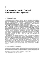
Instead of four variables, the solution of the coupled wave equations is simplified to
functions of two coefficients R
1
and S
2
. Suppose the corrugation inside the DFB laser
extends from z ¼ z

1
to z ¼ z
2
as shown in Fig. 4.2, the amplitude coefficients at the left and
the right facets can then be written as
Rðz
1
Þ¼R
1
e
gz
1
þ S
2
e
Àj
e
Àgz
1
ð4:6aÞ
Sðz
1
Þ¼R
1
e
j
e
gz
1
þ S

2
e
Àgz
1
ð4:6bÞ
Rðz
2
Þ¼R
1
e
gz
2
þ S
2
e
Àj
e
Àgz
2
ð4:6cÞ
Sðz
2
Þ¼R
1
e
j
e
gz
2
þ S

2
e
Àgz
2
ð4:6dÞ
From eqns (4.6a) and (4.6b), one can express R
1
and S
2
such that
R
1
¼
Sðz
1
Þe
Àj
À Rðz
1
Þ

2
À 1ðÞe
gz
1
ð4:7aÞ
S
2
¼
Rðz

1
Þe
j
À Sðz
1
Þ

2
À 1ðÞe
Àgz
1
ð4:7bÞ
Figure 4.2 A simplified schematic diagram for a 1-D corrugated DFB laser diode section.
104
TRANSFER MATRIX MODELLING IN DFB SEMICONDUCTOR LASERS
By substituting the above equations back into eqns (4.6c) and (4.6d), one obtains
Rðz
2
Þ¼
E À 
2
E
À1
1 À 
2
Rðz
1
ÞÀ
 E À E
À1

ðÞe
Àj
1 À 
2
Sðz
1
Þð4:8aÞ
Sðz
2
Þ¼
 E À E
À1
ðÞe
j
1 À 
2
Rðz
1
ÞÀ

2
E À E
À1
1 À 
2
Sðz
1
Þð4:8bÞ
where
E ¼ e

ðz
2
Àz
1
Þ
; E
À1
¼ e
Àðz
2
Àz
1
Þ
ð4:8cÞ
From the above equations, it is clear that the electric fields at the output plane z
2
can
be expressed in terms of the electric waves at the input plane. By combining the above
equations with eqn (4.2) we can relate the output and input electric fields through the
following matrix equation [6]
E
R
ðz
2
Þ
E
S
ðz
2
Þ

!
¼ T z
2
j z
1
ðÞÁ
E
R
ðz
1
Þ
E
S
ðz
1
Þ
!
¼
t
11
t
12
t
21
t
22
!
Á
E
R

ðz
1
Þ
E
S
ðz
1
Þ
!
ð4:9Þ
where matrix Tðz
2
j z
1
Þ represents any wave propagation from z ¼ z
1
to z ¼ z
2
and its
elements t
ij
ði; j ¼ 1; 2Þ are given as
t
11
¼
ðE À 
2
E
À1
ÞÁe

Àjb
0
ðz
2
Àz
1
Þ
ð1 À 
2
Þ
ð4:10aÞ
t
12
¼
ÀðE À E
À1
ÞÁe
Àj
e
Àjb
0
ðz
2
þz
1
Þ
ð1 À 
2
Þ
ð4:10bÞ

t
21
¼
ðE À E
À1
ÞÁe
j
e
jb
0
ðz
2
þz
1
Þ
ð1 À 
2
Þ
ð4:10cÞ
t
22
¼À
ð
2
E À E
À1
ÞÁe
jb
0
ðz

2
Àz
1
Þ
ð1 À 
2
Þ
ð4:10dÞ
For convenience, the matrix written in this way is called the forward transfer matrix because
the output plane at z ¼ z
2
is located further away from the origin. Similarly, waves
propagating inside the corrugated structure can also be expressed as the backward transfer
matrix such that [16]
E
R
ðz
1
Þ
E
S
ðz
1
Þ
!
¼ Uðz
1
j z
2
ÞÁ

E
R
ðz
2
Þ
E
S
ðz
2
Þ
!
¼
u
11
u
12
u
21
u
22
!
Á
E
R
ðz
2
Þ
E
S
ðz

2
Þ
!
ð4:11Þ
where matrix Uðz
1
j z
2
Þ represents any field propagation inside the section from z ¼ z
2
to
z ¼ z
1
. By comparing eqn (4.9) with eqn (4.11), it is obvious that
Uðz
1
j z
2
Þ¼ Tðz
2
j z
1
Þ½
À1
ð4:12Þ
BRIEF REVIEW OF MATRIX METHODS
105
where the superscript À1 denotes the inverse of the matrix. Due to conservation of energy,
both matrices Tðz
2

j z
1
Þ and Uðz
1
j z
2
Þ must satisfy the reciprocity rule such that their
determinants always give unity value [4]. In other words,
T
jj
¼ t
11
t
22
À t
12
t
21
¼ 1
U
jj
¼ u
11
u
22
À u
12
u
21
¼ 1

ð4:13Þ
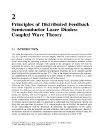
4.2.2 Introduction of Phase Shift (or Phase Discontinuity)
For a single PS DFB laser cavity as shown in Fig. 4.3, the phase shift at z ¼ z
2
divides the
laser cavity into two sections.
The field discontinuity is usually small along the plane of phase shift and any wave
travelling across the phase shift is assumed to be continuous. As a result, the transfer
matrices are linked up at the phase shift position as:
E
R
ðz
þ
2
Þ
E
S
ðz
þ
2
Þ
!
¼ P
ð2Þ
Á
E
R
ðz
À
2

Þ
E
S
ðz
À
2
Þ
!
¼
e
j
2
0
0e
Àj
2
!
Á
E
R
ðz
À
2
Þ
E
S
ðz
À
2
Þ

!
ð4:14Þ
where P
ð2Þ
is the phase-shift matrix at z ¼ z
2
; z
þ
2
and z
À
2
are the greater and lesser values of
z
2
, respectively, and 
2
corresponds to the phase change experienced by the electric waves
E
R
ðzÞ and E
S
ðzÞ. Alternatively, the physical phase shift of the corrugation may be used [9].
To avoid any confusion, we will use the phase shift of the electric wave hereafter.
On combining eqn (4.14) with the transfer matrix shown earlier in eqn (4.9), the overall
transfer matrix chain of a single-phase-shifted DFB laser becomes
E
R
ðz
3

Þ
E
S
ðz
3
Þ
"#
¼
t
ð2Þ
11
t
ð2Þ
12
t
ð2Þ
21
t
ð2Þ
22
2
4
3
5
Á
e
j
2
0
0e

Àj
2
"#
Á
t
ð1Þ
11
t
ð1Þ
12
t
ð1Þ
21
t
ð1Þ
22
2
4
3
5
Á
E
R
ðz
1
Þ
E
S
ðz
1

Þ
"#
¼ T
ð2Þ
Á P
ð2Þ
Á T
ð1Þ
Á
E
R
ðz
1
Þ
E
S
ðz
1
Þ
"#
ð4:15Þ
Figure 4.3 Schematic diagram showing a 1PS DFB laser diode section.
106
TRANSFER MATRIX MODELLING IN DFB SEMICONDUCTOR LASERS
Without affecting the results of the above equations, one can multiply a unity matrix I after
matrix T
(1)
. This matrix I behaves as if an imaginary phase shift of zero or a multiple of 2
has been introduced. As a result, the above matrix equation can be simplified such that
E

R
ðz
3
Þ
E
S
ðz
3
Þ
!
¼ Yðz
3
j z
1
ÞÁ
E
R
ðz
1
Þ
E
S
ðz
1
Þ
!
ð4:16Þ
where
Yðz
3

j z
1
Þ¼
Y
1
m¼2
F
ðmÞ
¼
y
11
z
3
j z
1
ðÞy
12
z
3
j z
1
ðÞ
y
21
z
3
j z
1
ðÞy
22

z
3
j z
1
ðÞ
!
ð4:17aÞ
F
ðmÞ
¼ T
ðmÞ
Á P
ðmÞ
¼
f
ðmÞ
11
f
ðmÞ
12
f
ðmÞ
21
f
ðmÞ
22
"#
¼
t
ðmÞ

11
e
j
m
t
ðmÞ
12
e
Àj
m
t
ðmÞ
21
e
j
m
t
ðmÞ
22
e
Àj
m
"#
ð4:17bÞ
P
ð1Þ
¼ I ¼
10
01
!

ð4:17cÞ
In the above equation, the overall matrix Yðz
3
j z
1
Þ comprises the characteristics of the field
propagation inside the DFB laser cavity, whilst the corrugated matrix T
ðmÞ
and the phase-
shift matrix P
ðmÞ
ðm ¼ 1; 2Þ are combined to form the matrix F
ðmÞ
.
The use of the transfer matrix method is not restricted to the corrugated DFB laser
structure. By modifying the values of  and  in the elements of the transfer matrix, other
structures like the planar Fabry–Perot structure, the planar waveguide structure and the
corrugated Distributed Bragg Reflector structure can also be represented using the transfer
matrix. A DBR structure is different from the DFB structure because DBR structures have
no underlying active region. The corrugated DBR structure simply acts as a partially
reflecting mirror, the amount of reflection depending on the wavelength. The maximum
reflection occurs near the central Bragg wavelength. Table 4.2 summarises all laser
structures that can be represented by transfer matrices. The differences between them are
also listed.
When the grating height g reduces to zero and the grating period  approaches infinity, the
feedback caused by the presence of corrugations becomes less important. At g ¼ 0, 
becomes zero as does the variable . When  becomes infinite, the detuning coefficient  is
reduced to the propagation constant 2n=. In this case, the DFB corrugated structure
becomes a planar structure. Following eqns (4.9) and (4.10), the transfer matrix equation of
Table 4.2 Laser structures that can be represented using the TMM

Structure Active layer Corrugation Comments
FP 38 ¼ 0 and >0
WG 88 ¼ 0 and  0
DFB 33finite  and >0
DBR 83finite  and  0
BRIEF REVIEW OF MATRIX METHODS
107
the planar structure becomes
E
R
ðz
2
Þ
E
S
ðz
2
Þ
!
¼ T
ð1Þ
Á
E
R
ðz
1
Þ
E
S
ðz

1
Þ
!
¼
t
ð1Þ
11
t
ð1Þ
12
t
ð1Þ
21
t
ð1Þ
22
"#
Á
E
R
ðz
1
Þ
E
S
ðz
1
Þ
!
ð4:18Þ

where
t
ð1Þ
11
¼ e
ðz
2
Àz
1
Þ
e
Àjbðz
2
Àz
1
Þ
t
ð1Þ
12
¼ t
ð1Þ
21
¼ 0
t
ð1Þ
22
¼ e
Àðz
2
Àz

1
Þ
e
jbðz
2
Àz
1
Þ
ð4:19Þ
In the above equation, the amplitude gain term  decides the characteristics of the planar
structure. For >0, the amplitude of the electric wave passing through will be amplified
and the structure will behave as if it is a laser amplifier. For  0, the amplitude of the
electric wave will either remain constant or be attenuated, as the planar structure becomes a
passive waveguide.
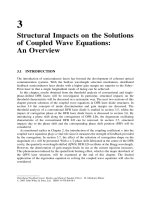
Similarly, the sign of  will decide whether a corrugated structure belongs to the DFB or
DBR type. By joining these matrices together as building blocks, one can extend the idea
further to form a general N-sectioned composite laser cavity as shown in Fig. 4.4. Laser
structures that comprise different combinations of the sections shown in Table 4.2 can be
modelled. By joining these matrices together appropriately, one ends up with
E
R
z
Nþ1
ðÞ
E
S
z
Nþ1
ðÞ
!

¼ F
ðNÞ
Á F
ðNÀ1Þ
ÁÁÁF
ð2Þ
Á F
ð1Þ
Á
E
R
z
1
ðÞ
E
S
z
1
ðÞ
!
¼ Yðz
Nþ1
j z
1
ÞÁ
E
R
z
1
ðÞ

E
S
z
1
ðÞ
!
ð4:20Þ
Figure 4.4 Schematic diagram of a general N-section laser cavity. The phase shifts f
1
;
2
; ...;
N
g
are shown. Active regions along the laser cavity are shaded.
108
TRANSFER MATRIX MODELLING IN DFB SEMICONDUCTOR LASERS