Tài liệu Laser điốt được phân phối thông tin phản hồi và các bộ lọc du dương quang P6 pdf

6
Above-Threshold Characteristics
of DFB Laser Diodes: A TMM
Approach
6.1 INTRODUCTION
The flexibility of the transfer matrix method allows one to evaluate the spectral behaviour of
a corrugated optical filter/amplifier and the threshold characteristic of a laser source. To
extend the analysis into the above-threshold biasing regime, the transfer matrix has to be
modified so as to include the dominant stimulated emission.
Based on a novel numerical technique, the above-threshold DFB laser model will be
presented in this chapter. Using a modified transfer matrix, the lasing mode characteristics of
DFB LDs will be determined. The new algorithm differs from many other numerical
methods in that no first-order derivative of the transfer matrix equation is necessary. As a
result, the same algorithm can be applied easily to other DFB laser structures with only
minor modification.
In section 6.2, the detail of the above-threshold laser model will be presented. Taking into
account the carrier rate equation, the dominant stimulated emission will be considered in
building the transfer matrix. The numerical algorithm behind the lasing model will be
discussed in section 6.3. Using the newly developed laser model, numerical results obtained
from various DFB lasers including QWS, 3PS and DCC structures will be shown in section
6.4. Longitudinally varying parameters such as the carrier concentration, photon density,
refractive index and the internal field intensity distributions will be presented with respect to
biasing current changes. Impacts due to the structural variation in particular will be discussed.
6.2 DETERMINATION OF THE ABOVE-THRESHOLD
LASING MODE USING THE TMM
In above-threshold analysis, the lasing wavelength and the optical output power are
important. For laser devices to be used in coherent communication systems, the single-mode
stability and the spectral linewidth should also be considered. Provided that the longitudinal
distributions of the carrier, photons and other parameters are known, one can include the
Distributed Feedback Laser Diodes and Optical Tunable Filters H. Ghafouri–Shiraz
# 2003 John Wiley & Sons, Ltd ISBN: 0-470-85618-1

spatial hole burning effect as well as the non-linear gain [1] in the above-threshold analysis.
From the threshold characteristic of a DFB LD, a quasi-uniform gain model has been
proposed using the perturbation technique [2]. However, in the analysis, a uniform gain
profile along the cavity and a linear peak gain model were assumed. Using the TMM [3], the
uniform gain profile was later improved by introducing a longitudinal dependence of gain
along the cavity and an approximated carrier density was obtained for each sub-section
under a fixed biasing current. With the laser cavity represented by such a small number of
sub-sections, impacts due to the localised SHB effect can only be shown in an approximate
manner. For a more realistic laser model, effects of SHB and any other non-linear gain
saturation have to be considered.
In the last chapter, the flexibility of the TMM allowed us to evaluate a DFB laser design
quickly, based on the threshold analysis. However, TMM fails to predict the above-threshold
lasing characteristics after the lasing threshold condition is reached and stimulated photons
become dominant. To take into account any change of injection current, it is necessary to
include the carrier rate equation in the analysis. In this section, the relationship between the
injection current (or carrier concentration) and the elements of the transfer matrix (mainly
amplitude gain  and detuning factor ) will be presented. From the output electric field
obtained from the overall transfer matrix, the optical output power will then be evaluated. To
include the localised effect in the TMM, a larger number of transfer matrices have to be used
so that the length represented by each transfer matrix becomes much smaller. From the N-
sectioned DFB laser model, physical parameters such as the carrier concentration and
photon concentration are assumed to be homogeneous within an arbitrary sub-section. As a
result, information such as the localised carrier and photon concentrations are obtained from
each transfer matrix. Consequently, longitudinal distributions of the lasing mode carrier
density, photon density, refractive index and the internal field distribution are obtained.
According to Chapter 4, the transfer matrix of an arbitrary section k as shown in Fig. 6.1
can be expressed as
E
R
ðz

kþ1
Þ
E
S
ðz
kþ1
Þ
!
¼ F z
kþ1
j z
k
ðÞÁ
E
R
ðz
k
Þ
E
S
ðz
k
Þ
!
¼
f
11
f
12
f

21
f
22
!
Á
E
R
ðz
k
Þ
E
S
ðz
k
Þ
!
ð6:1Þ
Figure 6.1 Schematic diagram showing a general section in a DFB LD cavity. 
k
shows the phase
shift between sections k and k À 1.
150
ABOVE-THRESHOLD CHARACTERISTICS OF DFB LASER DIODES
where Fðz
kþ1
j z
k
Þ is the transfer matrix of the corrugated section between z ¼ z
k
and z

kþ1
whilst its elements f
ij
ði; j ¼ 1; 2Þ are given as
f
11
¼
ðE À &
2
E
À1
ÞÁe
Àjb
0
ðz
kþ1
Àz
k
Þ
e
j
k
1 À &
2
ðÞ
ð6:2aÞ
f
12
¼
À& E À E

À1
ðÞÁe
Àj
e
Àjb
0
z
kþ1
þz
k
ðÞ
e
Àj
k
1 À &
2
ðÞ
ð6:2bÞ
f
21
¼
& E À E
À1
ðÞÁe
j
e
jb
0
z
kþ1

þz
k
ðÞ
e
j
k
1 À &
2
ðÞ
ð6:2cÞ
f
22
¼
Àð&
2
E À E
À1
ÞÁe
jb
0
ðz
kþ1
Àz
k
Þ
e
Àj
k
1 À &
2

ðÞ
ð6:2dÞ
where  is the residue corrugation phase at z ¼ 0 and 
k
is the phase discontinuity between
section k and k À 1. Other parameters used are defined as
E ¼ e
gðz
kþ1
Àz
k
Þ
; E
À1
¼ e
Àgðz
kþ1
Àz
k
Þ
ð6:3aÞ
& ¼
j
 À j þ g
ð6:3bÞ
For DFB lasers having a fixed cavity length, one must determine both the amplitude gain
coefficient  and the detuning coefficient  of the section k in order that each matrix element
f
ij
ði; j ¼ 1; 2Þ as shown in eqn (6.2) can be determined. For first-order Bragg diffraction, it

was shown in Chapter 2 that  and  can be expressed as:
 ¼
À g À 
loss
2
ð6:4Þ
 ¼
2p
!
n À
2pn
g
!!
B
ð! À !
B
ÞÀ
p
Ã
ð6:5Þ
where À is the optical confinement factor, g is the material gain, 
loss
includes the absorption
in both the active and the cladding layer as well as any scattering loss. In eqn (6.5), n is the
refractive index of section k and !
B
is the Bragg wavelength. To take into account any
dispersion due to the difference between the actual wavelength and the Bragg wavelength
[4], the group refractive index n
g

is included in eqn (6.5). In Chapter 2, it was shown that the
material gain g of a bulk semiconductor device can be expressed as
g ¼ A
0
ðN À N
0
ÞÀA
1
! À !
0
À A
2
N À N
0
ðÞðÞ½
2
ð6:6Þ
where a parabolic model is assumed. In this equation, A
0
is the differential gain, N
0
is the
transparency carrier concentration and !
0
is the wavelength of the peak gain at transparency
gain (i.e. g ¼ 0). The variable A
1
in eqn (6.6) determines the base width of the gain spectrum
and A
2

corresponds to any change associated with the shift of the peak wavelength. Using a
first-order approximation for the refractive index n, we obtain
n ¼ n
ini
þ À
@n
@N
N ð6:7Þ
DETERMINATION OF THE ABOVE-THRESHOLD LASING MODE USING THE TMM
151
In the above equation, n
ini
is the effective refractive index at zero carrier injection, À is the
optical confinement factor and @n=@N is the differential index. For a symmetrical double
heterostructure laser having an active laser width of w and thickness d [5], n
ini
is
approximated as
n
2
ini
% n
2
act
À X log
10
1 þ n
2
act
À n

2
clad
ÀÁ
=X
ÂÃ
ð6:8Þ
where
X ¼
!
2
B
2p
2
d
2
ð6:9Þ
In eqn (6.8), a single transverse and lateral mode are assumed n
act
and n
clad
are the refractive
indices of the active and the cladding layer, respectively. From eqns (6.6) and (6.7), it is clear
that both g and n are related to the carrier concentration N. As mentioned in Chapter 2, the
carrier concentration N and the stimulated photon density S are coupled together through the
steady-state carrier rate equation ð@N=@t ¼ 0Þ which is shown here as
I
qV
¼ R þ R
st
ð6:10Þ

where
R ¼
N
(
þ BN
2
þ CN
3
ð6:11aÞ
R
st
¼
v
g
gS
1 þ "S
ð6:11bÞ
In the above equations R
st
is the stimulated emission rate per unit volume and R is the rate of
other non-coherent carrier recombinations. Other parameters used are as follows: I is the
injection current, q is the electronic charge and V is the volume of the active layer, ( is
the linear recombination lifetime, B is the radiative spontaneous emission coefficient, C is
the Auger recombination coefficient and v
g
¼ c=n
g
is the group velocity. To include any
non-linearity and saturation effects, a non-linear coefficient " has been introduced [6]. For
strongly index-guided semiconductor structures like the buried heterostructure, the lasing

mode is confined through the total internal reflection that occurs at the active and cladding
layer interfaces. Both the active layer width w and thickness d are usually small compared
with the diffusion length. As a result, the carrier density does not vary significantly along the
transverse plane of the active layer dimensions and the carrier diffusion term in the carrier
rate equation has been neglected [7]. In an index-coupled DFB laser cavity, the local photon
density inside the cavity can be expressed [8] as
SðzÞ%
2"
0
nðzÞn
g
!
hc
Á c
2
0
E
R
ðzÞ
jj
2
þ E
S
ðzÞ
jj
2
hi
ð6:12Þ
where "
0

¼ 8:854 Â 10
À12
Fm
À1
is the free space electric constant. From the escaping
photon density at the output facet, the output power is then determined as
Pðz
j
Þ¼
dw
À
v
g
hc
!
Sðz
j
Þð6:13Þ
152
ABOVE-THRESHOLD CHARACTERISTICS OF DFB LASER DIODES
According to the general N-sectioned DFB laser cavity model, j ¼ 1 and j ¼ N þ 1
correspond to the power output at the left and right facets, respectively. In eqn (6.12), c
0
is a
dimensionless coefficient that determines the total electric field
"
EðzÞ as
"
EðzÞ¼c
0

EðzÞ¼c
0
E
R
ðzÞþE
S
ðzÞ½ ð6:14Þ
where E
R
ðzÞ and E
S
ðzÞ are the normalised electric field components as shown in eqn (4.40).
Using the forward transfer matrix, it is important that both travelling electric fields E
R
ðzÞ and
E
S
ðzÞ are normalised at the left facet ðz ¼ z
1
Þ as
E
R
ðz
1
Þ
jj
2
þ E
S
ðz

1
Þ
jj
2
¼ 1 ð6:15Þ
Of course, both E
R
ðz
1
Þ and E
S
ðz
1
Þ should satisfy the boundary condition at the left facet such
that
E
R
ðz
1
Þ
E
S
ðz
1
Þ
¼
^
r
1
ð6:16Þ

From the threshold analysis, both the amplitude threshold gain 
th
and detuning coefficient

th
are determined. With virtually negligible numbers of coherent photons at the laser
threshold, the threshold carrier concentration N
th
can be determined from eqns (6.4) and
(6.6) such that
N
th
¼ N
0
þ 
loss
þ 2
th
ðÞ=À A
0
ð6:17Þ
where peak gain is assumed at threshold with A
1
¼ A
2
¼ 0. Consequently, the refractive
index at threshold can be found to be
n
th
¼ n

ini
þ À
@n
@N
N
th
ð6:18Þ
By substituting  ¼ 
th
in eqn (6.5) at the threshold condition, the threshold wavelength !
th
can be obtained
!
th
¼
2p!
B
n
th
þ n
g
ÀÁ

th
!
B
þ 2pn
g
þ !
B

p=Ã
ð6:19Þ
Consequently, the peak gain wavelength at zero gain transparency is found from eqn (6.6) to be
!
0
¼ !
th
þ A
2
ðN
th
À N
0
Þð6:20Þ
In the next section, features of the numerical process that help to determine the above-
threshold characteristics will be discussed in a systematic way.
6.3 FEATURES OF NUMERICAL PROCESSING
To evaluate the longitudinal distribution of the carriers and the photons in the analysis, a
large number of transfer matrices must be used. For a 500 mm long QWS DFB laser, at least
5000 transfer matrices have been adopted to evaluate the above-threshold characteristics. To
FEATURES OF NUMERICAL PROCESSING
153
characterise the oscillation mode for such a non-uniform system, a numerical method such
as the Newton–Raphson method will not be appropriate since it is almost impossible to find
the required first-order derivative. The situation becomes worse when one realises that the
oscillation characteristic depends on the laser structure.
In the analysis, a novel numerical technique has been developed. Using this numerical
technique, it is not necessary to find any first-order derivative. In addition, the algorithm has
been designed such that with only minor changes, it can be implemented easily in the design
of various DFB laser structures. At a fixed above-threshold current, initial guesses for the

lasing wavelength ! and the dimensionless coefficient c
0
are chosen. By matching the
boundary condition at the right facet, lasing characteristics such as the carrier density,
photon density, refractive index distribution, optical output power and the lasing wavelength
can be evaluated. Consequently, information such as the single-mode stability and the
spectral linewidth can be determined.
In Fig. 6.2, a flowchart helps to explain the numerical procedure. Features of the novel
numerical technique are highlighted as follows [9]:
1. For a DFB laser diode with a specific structural design (e.g. a QWS, 3PS or a DCC DFB
LD), the oscillation condition at the lasing threshold is first determined. Numerical
methods like the Newton–Raphson method are applied to determine the threshold
characteristic. A reasonable number of roots near the Bragg wavelength are found on
the complex plane. Each root ð
th
;
th
Þ that represents an oscillation mode is sorted in
rising order of 
th
. The one showing the smallest 
th
will become the lasing mode after
the threshold condition is reached.
2. Using eqns (6.17)–(6.20), N
th
, n
th
, !
th

and !
0
are evaluated from the threshold value of
ð
th
;
th
Þ. Since there are virtually no stimulated photons at the lasing threshold
condition, the threshold current I
th
is determined using eqn (6.10).
3. The DFB laser cavity is then subdivided into a large number of sections each
represented by a transfer matrix.
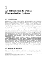
4. An injection current that is normalised with respect to the threshold current is specified.
To start the iteration, values of ! and c
0
are given as initial guesses such that a
mathematical grid as shown in Fig. 6.3 is built. Each intersection point on the grid
(25 points all together) represents a pair of (c
0
, !) that will be used in the iteration.
5. Using the forward transfer matrix, the photon density at the inner left facet is first
determined. With no information on the carrier concentration, the threshold refractive
index n
th
is assumed. The carrier concentration N at the left facet is then found using
eqn (6.10), and subsequently input components E
R
ðz
1

Þ and E
S
ðz
1
Þ are obtained
according to eqns (6.15) and (6.16).
6. At this stage, the photon density at the left facet can be found using eqn (6.12). The
carrier concentration is then evaluated by solving the carrier rate equation that includes
the multi-carrier recombination. Subsequently, both  and  of the first section and
matrix elements f
ij
ði; j ¼ 1; 2Þ of the first matrix are determined.
7. Using the newly formed transfer matrix, the electric field at the output plane can be
evaluated and hence the output photon density found. Both  and  of the following
section are then found and a new transfer matrix is formed. The whole process is then
154
ABOVE-THRESHOLD CHARACTERISTICS OF DFB LASER DIODES
Figure 6.2 Flow chart showing the procedures in the numerical algorithm.
repeated until the output plane of the transfer matrix has reached the right facet. The
discrepancy with the boundary condition is evaluated and stored (min_err).
8. By repeating the same calculation for all other (c
0
, !) pairs obtained from the
mathematical grid, the pair showing the smallest discrepancy will be selected.
Depending on the position of the final point on the mathematical grid (it may be along
the boundary, at the corner or near the centre), a new mathematical grid will be created.
Possible quantisation error must be considered when forming the new mathematical grid.
9. Procedures (5) to (8) should be repeated until the boundary condition falls within a
discrepancy of <10
À14

or the iterative change of wavelength ðÁ!Þ falls below 10
À17
m.
The final pair (c
0
, !)
final
is then stored.
10. The above-threshold characteristic of the DFB laser is determined by passing the
(c
0
, !)
final
pair once again through the transfer matrix chain. From the photon density
obtained at both facets, the output optical power is obtained. From each transfer matrix,
the lasing mode distribution of the carrier concentration N(z), photon density SðzÞ,
refractive index nðzÞ, amplitude gain ðzÞ and detuning coefficient ðzÞ can be evaluated.
11. The average values of
"

L
and
"

L
associated with the lasing mode are then obtained from
the corresponding longitudinal distribution as
"

L

¼
P
N
j¼1

j
N
ð6:21Þ
"

L
¼
P
N
j¼1

j
N
ð6:22Þ
where N is the total number of transfer matrices used and 
j
and 
j
( j ¼ 1toN) are the
Figure 6.3 A5Â 5 mathematical grid used in the above-threshold analysis.
156
ABOVE-THRESHOLD CHARACTERISTICS OF DFB LASER DIODES