Tài liệu Laser điốt được phân phối thông tin phản hồi và các bộ lọc du dương quang P8 doc
Bạn đang xem bản rút gọn của tài liệu. Xem và tải ngay bản đầy đủ của tài liệu tại đây (461.2 KB, 35 trang )
8
Circuit and Transmission-Line
Laser Modelling (TLLM)
Techniques
8.1 INTRODUCTION
Although today microwave and optical engineering appear to be separate disciplines, there
has been a tradition of interchange of ideas between them. In fact, many traditional
microwave concepts have been adapted to yield optical counterparts. The laser, as an optical
device that plays a key role in optoelectronics and fibre-optic communications, grew from
the work of its microwave predecessor, the maser (microwave amplification by stimulated
emission of radiation) [1]. The operating principle behind the laser is very similar to that of
the microwave oscillator. In a semiconductor laser, the required feedback may either be
provided by the cleaved facets of Fabry–Perot lasers or by a periodic grating in distributed
feedback lasers. The optical technique of injection locking of lasers by external light [2] is
an idea borrowed from the phenomenon of injection locking of microwave oscillators by an
external electronic signal [3]. The close relationship between optical and microwave
principles suggests that it may be advantageous to apply microwave circuit techniques in
modelling of semiconductor lasers.
Engineers work best when using tools they are familiar with. In particular, electrical and
electronic engineers are familiar with well-established electrical circuit models as tools to
aid themselves in the understanding and prediction of behaviour of electrical machines or
electronic devices. Since the early days of radio frequency (RF) and microwave engineering,
microwave circuit theory has allowed us to explore fundamental properties of
electromagnetic waves by giving us an intuitive understanding of them without the need
to invoke detailed and rigorous electromagnetic field theories [4–5]. In the same spirit,
microwave circuit formulation of the semiconductor laser diode enhances our understanding
of the device, which is otherwise obscured by hard-to-visualise mathematical formulations.
Complex mathematical models are too sophisticated to be desirable for engineers, especially
those who are not specialists in the field of laser physics but would like to have a quick-to-
digest method of understanding and designing semiconductor laser devices. It is far more
convenient to work in terms of voltages, currents and impedances. In fact, electromagnetic
field theory and distributed-element circuits (transmission lines) give identical solutions
Distributed Feedback Laser Diodes and Optical Tunable Filters H. Ghafouri–Shiraz
# 2003 John Wiley & Sons, Ltd ISBN: 0-470-85618-1
when we are dealing with transverse electromagnetic (TEM) fields, where voltages and
currents in the transmission lines are uniquely related to the transverse electric and magnetic
fields, respectively.
The attractiveness of using equivalent circuit models for semiconductor laser devices
stems from their ability to provide an analogy of laser theory in terms of microwave circuit
principles. In addition, microwave circuit models of laser diodes are compatible with
existing circuit models of microwave devices such as heterojunction bipolar transistors
(HBTs) and field-effect transistors (FETs) – an attractive feature for optoelectronic integrated
circuit (OEIC) design [6]. Equivalent circuit models have effectively helped many to
understand, design and optimise integrated circuits (ICs) in the microelectronics industry
and they have the potential to do the same for the optoelectronics industry. The main theme
of this chapter is microwave circuit modelling techniques applied to semiconductor laser
devices.
Two types of microwave circuit model for semiconductor lasers have been investigated:
the simple lumped-element model based on low-frequency circuit concepts and the more
versatile distributed-element model based on transmission-line modelling. The former
(lumped-element circuit model) is based on the simplifying assumption that the phase of
current or voltage across the dimension of the components has little variation. This is true
when considering only the modulated signal instead of the optical carrier signal. In this case,
Kirchoff’s law can be applied, which is nothing more than a special case of Maxwell’s
equations [7–8]. Strictly speaking, laser devices have dimensions in the order of the
operating wavelength, thus lumped-element models may not be suitable in ultrafast
applications where propagation plays an important role such as in active mode locking [9].
However, the lumped-element circuit is reasonably accurate for microwave applications if
all the important processes and effects are modelled accordingly by the circuit on an
equivalence basis.
The latter of the two circuit modelling techniques (i.e. transmission-line modelling) is a
more powerful circuit model that includes distributed effects, which will be discussed in
detail in this chapter. It is worth pointing out that at microwave frequencies and above,
voltmeters and ammeters for direct measurement of voltages and currents do not exist, so
voltage and current waves are only introduced conceptually in the microwave circuit to
make optimum use of the low-frequency circuit concepts.
8.2 THE TRANSMISSION-LINE MATRIX (TLM) METHOD
The transmission-line matrix (TLM) was originally developed to model passive microwave
cavities by using meshes of transmission lines [9–10]. The numerical processes involved in
TLM resemble the mechanism of wave propagation but they are discretised in both time and
space [10–11]. Much work has been carried out using the TLM method for analysis of
passive microwave waveguide structures (see [12] and references therein). Most of the work
done involved two-dimensional and three-dimensional TLMs, with the exception of the
application to lumped networks [13–14], the heat diffusion problem [15] and semiconductor
laser modelling [16]. Although the TLM is unconditionally stable when modelling passive
devices, the semiconductor laser is an active device and therefore requires more careful
consideration. The basics of the one-dimensional (1-D) TLM will be presented in the
following section, which forms the basis of the transmission-line laser model (TLLM) [17].
196
CIRCUIT AND TRANSMISSION-LINE LASER MODELLING (TLLM) TECHNIQUES
8.2.1 TLM Link Lines
The TLM is a discrete-time model of wave propagation simulated by voltage pulses
travelling along transmission lines. The medium of propagation is represented by the
transmission lines – a general or lossy transmission line consists of series resistance, shunt
admittance, series inductance and shunt capacitance per unit length, whereas an ideal or
lossless transmission line has reactive elements only. The transmission line may be described
by a set of telegraphist equations [7], which can be shown to be equivalent to Maxwell’s
equations. There are two types of TLM element that can be used as the building blocks of a
complete TLM network – they are the TLM stub lines and link lines [13]. For a lossless
transmission line, the velocity of propagation is expressed by
v
p
¼
1
ffiffiffiffiffiffiffiffiffiffi
L
d
C
d
p
¼
Ál
Át
ð8:1Þ
where L
d
is inductance per unit length, C
d
is capacitance per unit length, Ál is the unit
section length, and Át is the model time step. In Fig. 8.1, it is shown that a lumped series
inductor (L) is equivalent to a transmission line with inductance per unit length of L
d
, where
[13]
L ¼ L
d
Ál ð8:2Þ
The characteristic impedance Z
0
ðÞof the transmission line can be found from
Z
0
¼
ffiffiffiffiffiffi
L
d
C
d
r
¼
L
Át
ð8:3Þ
However, there is a small error associated with the shunt capacitance of the transmission
line, which can be expressed as
C
e
¼
ðÁtÞ
2
L
ð8:4Þ
Figure 8.1 TLM link-lines.
THE TRANSMISSION-LINE MATRIX (TLM) METHOD
197
Similarly, the lumped shunt capacitor (C) is equivalent to a transmission line with
capacitance per unit length of C
d
(Fig. 8.1) where
C ¼ C
d
Ál ð8:5Þ
The characteristic impedance Z
0
ðÞof the line can be expressed by [13]
Z
0
¼
Át
C
ð8:6Þ
and the associated error in the form of a series inductor is given by
L
e
¼
ÁtðÞ
2
C
ð8:7Þ
The errors C
e
and L
e
are of the order of ÁtðÞ
2
and can be reduced by using a smaller
model time step. In practice, there is no component that is purely inductive nor purely
capacitive. The parasitic errors can therefore be adjusted by changing the time step ÁtðÞto
model stray inductance or capacitance. If two adjacent reactive elements are required, then
the parasitic error from one line can be ‘absorbed’ into its adjacent line so that the parasitic
error may be eliminated for at least one of the lines.
8.2.2 TLM Stub Lines
In the preceding section, we saw how lumped reactive elements can be simulated by TLM
link lines. The lumped reactive elements may also be modelled by TLM stub lines, as shown
in Fig. 8.2. The lumped inductor L is also equivalent to a short-circuit stub with a
characteristic impedance of [13]
Z
0
¼
2L
Át
ð8:8Þ
Figure 8.2 TLM stub lines.
198
CIRCUIT AND TRANSMISSION-LINE LASER MODELLING (TLLM) TECHNIQUES
and has a parasitic capacitance expressed by
C
e
¼
ðÁtÞ
2
4L
ð8:9Þ
On the other hand, the lumped capacitor is equivalent to an open-circuit stub with
characteristic impedance of [13]
Z
0
¼
Át
2C
ð8:10Þ
and has a parasitic inductance expressed by
L
e
¼
ðÁtÞ
2
4C
ð8:11Þ
For TLM stub lines, the length of the transmission line is chosen such that it takes half a
model time step Át=2ðÞfor the pulse to travel from one end to another (see Fig. 8.2). The
reason is to allow the voltage pulses to propagate to the termination of the stub and back
again at the scattering node in one complete time iteration ÁtðÞ. This way, all incident
voltage pulses will arrive at their scattering nodes in exactly the same time, irrespective of
stub lines or link lines, i.e. the voltage pulses are synchronised.
8.3 SCATTERING AND CONNECTING MATRICES
The most basic algorithm of TLM involves two main processes: scattering and connecting.
When the incident voltage pulses, V
i
, arrive at the scattering node, they are operated by a
scattering matrix and reflected voltage pulses, V
r
, are produced. These reflected pulses then
continue to propagate along the transmission lines and become incident pulses at adjacent
scattering nodes – this process is described by the connecting matrix. Formally, the TLM
algorithm may be expressed as
k
V
rT
¼ S
k
V
iT
½Scattering
kþ1
V
iT
¼ C
k
V
rT
½Connecting
ð8:12Þ
The terms V
iT
and V
rT
are the transpose matrices of the incident and reflected pulses,
respectively. The terms k and k þ 1 denote the kth and ðk þ 1Þth time iteration, respectively.
The scattering and connecting matrices are denoted by S and C, respectively. As the matrices
involved in eqn (8.12) depend on the type of TLM sub-network, a worked example based on
the TLM sub-network of Fig. 8.3 follows.
The TLM sub-network consists of three ‘branches’ of lossy transmission lines as shown in
Fig. 8.3, where scattering and connecting of the voltage pulses are clearly described
pictorially. The normalised impedances are unity for the two lines connected to adjacent
SCATTERING AND CONNECTING MATRICES
199
Figure 8.3 The TLM stub line: (a) incident pulses arriving at scattering node; (b) incident pulses
scattered into reflected pulses (scattering); (c) reflected pulses arriving at adjacent nodes (connecting).
200
CIRCUIT AND TRANSMISSION-LINE LASER MODELLING (TLLM) TECHNIQUES
nodes and Z
s
for the remaining branch (open–circuit stub line). The associated normalised
resistances are R and R
s
, respectively. The matrices V
iT
and V
rT
are given as
V
rT
¼
V
1
V
2
V
3
2
4
3
5
r
V
iT
¼
V
1
V
2
V
3
2
4
3
5
i
ð8:13Þ
where V
1
, V
2
and V
3
are the voltage pulses on ports 1, 2, and 3, respectively on each
scattering node (see Fig. 8.3). The superscripts r and i denote reflected and incident
pulses, respectively. It is convenient to break up the scattering matrix S and express it as
[15–19]
S ¼ p  q À r ð8:14Þ
where the matrices p, q, and r are defined in the following. For the type of TLM sub-network
in Fig. 8.3, we have
q ¼ q
1
q
2
q
3
½
where
q
i
¼
2ðR
s
þ Z
s
Þ
1 þ R þ 2ðR
s
þ Z
s
Þ
i ¼ 1; 2
2ð1 þ RÞ
1 þ R þ 2ðR
s
þ Z
s
Þ
i ¼ 3
8
>
>
>
<
>
>
>
:
ð8:15Þ
The matrix q may be found by replacing the sub-network by its Thevenin-equivalent circuit,
which is shown in Fig. 8.4. By definition of the voltage pulse, V
i
x
[5], its generator or source
Figure 8.4 Thevenin equivalent circuit of the TLM sub-network.
SCATTERING AND CONNECTING MATRICES
201
require a value of 2V
i
x
, where x denotes the port number (1, 2 or 3). The nodal voltage vðÞ
can be defined as
v ¼ q
k
V
iT
ð8:16Þ
This will be explained further by using two simple TLM sub-networks as examples later.
The matrix p is found by applying the voltage division rule and is given as
p ¼ p
1
p
2
p
3
½
T
where
p
i
¼
1
1 þ R
i ¼ 1; 2
Z
s
R
s
þ Z
s
i ¼ 3
8
>
>
>
<
>
>
>
:
ð8:17Þ
and the matrix r is given by
r ¼
r
11
00
0 r
22
0
00r
33
2
4
3
5
where
r
ii
¼
1 À R
1 þ R
i ¼ 1; 2
Z
s
À R
s
R
s
þ Z
s
i ¼ 3
8
>
>
>
<
>
>
>
:
ð8:18Þ
If lossless transmission lines are used, we have R ¼ R
s
¼ 0, and eqns (8.15), (8.17) and
(8.18) become
q ¼ q
1
q
2
q
3
½ ð8:19aÞ
q
i
¼
2Z
s
1 þ 2Z
s
i ¼ 1; 2
2
1 þ 2Z
s
i ¼ 3
8
>
>
<
>
>
:
ð8:19bÞ
p ¼
1
1
1
2
6
4
3
7
5
ð8:19cÞ
r ¼
100
010
001
2
6
4
3
7
5
ð8:19dÞ
202
CIRCUIT AND TRANSMISSION-LINE LASER MODELLING (TLLM) TECHNIQUES
The connecting matrix depends on how the transmission lines are connected, that is, which
port(s) of one scattering node is/are connected to which port(s) of other adjacent scattering
node(s). The matrix element in the connecting matrix is unity only if a connection allows a
pulse to travel from port i of node m to port j of node n. In the example given in Fig. 8.3, the
connecting matrix C may be expressed by 3 Â 3 elements, where we have pulses travelling
from
1. port 2 of node nÀ 1 to port 1 of node n
2. port 3 of node n to port 3 of node n (open-circuit stub)
3. port 1 of node n þ 1 to port 2 of node n
Thus, the connecting matrices for node n and its adjacent nodes n À 1 and n þ 1 are given as
C
nÀðnÀ1Þ
¼
000
100
000
2
4
3
5
C
nÀn
¼
000
000
001
2
4
3
5
C
nÀðnþ1Þ
¼
010
000
000
2
4
3
5
ð8:20Þ
A simple example of another TLM sub-network is shown in Fig. 8.5(a), which consists of a
resistor ‘sandwiched’ between two lossless transmission lines. In the Thevenin equivalent
circuit shown in Fig. 8.5(b), each transmission line is replaced by its characteristic
impedance in series with a voltage generator of twice the incident voltage pulse. The
Figure 8.5 (a) A TLM sub-network and (b) its Thevenin equivalent circuit.
SCATTERING AND CONNECTING MATRICES
203
incident voltage pulses are denoted as V
i
1
and V
i
2
, while the reflected pulses are V
r
1
and V
r
2
.
The impedances of the lossless transmission lines are Z
1
and Z
2
. From Fig. 8.5(b), the nodal
voltages (v
1
and v
2
) may be expressed as
v
1
¼
i
1
Y
1
v
2
¼
i
2
Y
2
ð8:21Þ
where
i
1
¼
2V
i
1
Z
1
þ
2V
i
2
R þ Z
2
ðÞ
i
2
¼
2V
i
1
R þ Z
1
ðÞ
þ
2V
i
2
Z
2
ð8:22Þ
and
Y
1
¼
1
Z
1
þ
1
R þ Z
2
Y
2
¼
1
Z
2
þ
1
R þ Z
1
ð8:23Þ
By substituting eqns (8.22) and (8.23) into (8.21), we have
v
1
¼
1
R þ Z
1
þ Z
2
2ðR þ Z
2
ÞV
i
1
þ 2Z
1
V
i
2
ÂÃ
v
2
¼
1
R þ Z
1
þ Z
2
2Z
2
V
i
1
þ 2ðR þ Z
1
ÞV
i
2
ÂÃ
ð8:24Þ
By the original definition of the nodal voltage [5], we have the relationships
v
1
¼ V
i
1
þ V
r
1
v
2
¼ V
i
2
þ V
r
2
ð8:25Þ
Now we can write down the reflected voltage pulses in terms of the incident pulses as
V
r
1
¼ v
1
À V
i
1
V
r
1
¼
1
R þ Z
1
þ Z
2
ðR À Z
1
þ Z
2
ÞV
i
1
þ 2Z
1
V
i
2
ÂÃ
ð8:26Þ
and
V
r
2
¼ v
2
À V
i
2
V
r
2
¼
1
R þ Z
1
þ Z
2
2Z
2
V
i
1
þðRÀ Z
2
þ Z
1
ÞV
i
2
ÂÃ
Finally, the complete scattering matrix of the TLM network in Fig. 8.5 at the kth iteration is
expressed by [13]
S
k
¼
1
R þ Z
1
þ Z
2
ðR À Z
1
þ Z
2
Þ 2Z
1
2Z
2
ðR À Z
2
þ Z
1
Þ
!
ð8:27Þ
204
CIRCUIT AND TRANSMISSION-LINE LASER MODELLING (TLLM) TECHNIQUES
Another simple but useful TLM sub-network is shown in Fig. 8.6(a) and its Thevenin
equivalent is given in Fig. 8.6(b). This is similar to one of the sub-networks in Fig. 8.3 but it
is lossless in this case and each branch has a different value of line impedance. Now, the
common nodal current is defined by
i ¼
2V
i
1
Z
1
þ
2V
i
2
Z
2
þ
2V
i
3
Z
3
ð8:28Þ
From Fig. 8.6(b), the total admittance at the scattering node is expressed as
Y ¼
1
Z
1
þ
1
Z
2
þ
1
Z
3
Y ¼
Z
2
Z
3
þ Z
1
Z
2
þ Z
1
Z
3
Z
1
Z
2
Z
3
ð8:29Þ
Figure 8.6 (a) A TLM sub-network and (b) its Thevenin equivalent circuit.
SCATTERING AND CONNECTING MATRICES
205
From Millman’s thereom [19] the common nodal voltage can be found from
v ¼
i
Y
¼
2Z
2
Z
3
V
i
1
þ 2Z
1
Z
2
V
i
3
þ 2Z
1
Z
3
V
i
2
Z
2
Z
3
þ Z
1
Z
2
þ Z
1
Z
3
ð8:30Þ
Since the sum of incident voltage pulse and reflected pulse gives the nodal voltage, see
eqn (8.25), the reflected pulse may again be found by subtracting the incident pulse from the
nodal voltage, that is
V
r
1
¼ v À V
i
1
V
r
1
¼
2Z
2
Z
3
V
i
1
þ 2Z
1
Z
2
V
i
3
þ 2Z
1
Z
3
V
i
2
Z
2
Z
3
þ Z
1
Z
2
þ Z
1
Z
3
À V
i
1
V
r
1
¼
ðZ
2
Z
3
À Z
1
Z
2
À Z
1
Z
3
ÞV
i
1
þ 2Z
1
Z
2
V
i
3
þ 2Z
1
Z
3
V
i
2
Z
2
Z
3
þ Z
1
Z
2
þ Z
1
Z
3
ð8:31Þ
In a similar manner, the reflected pulses, V
r
2
and V
r
3
, can also be found, and the complete
scattering matrix of the sub-network in Fig. 8.6 is expressed by
S
k
¼
Z
2
Z
3
À Z
1
Z
2
À Z
1
Z
3
2Z
1
Z
2
2Z
1
Z
3
2Z
2
Z
3
Z
1
Z
2
À Z
2
Z
3
À Z
1
Z
3
2Z
1
Z
3
2Z
2
Z
3
2Z
1
Z
2
Z
1
Z
3
À Z
2
Z
3
À Z
1
Z
2
2
4
3
5
Z
1
Z
2
þ Z
1
Z
3
þ Z
2
Z
3
ð8:32Þ
The TLM sub-network in Fig. 8.6(a) forms the basis of the matching network. There are
many other TLM sub-networks that can be formed by using series and shunt resistors
together with the TLM link lines and stub lines. For example, periodically unmatched
boundaries of TLM link lines can be used to mimic corrugated gratings [20] and shunt
conductances can be included to model gain-coupled DFB lasers [21]. A TLM sub-network
which consists of a series resistor and two reactive stub lines will now be used to model the
wavelength dependence of semiconductor laser gain in the transmission-line laser model.
8.4 TRANSMISSION-LINE LASER MODELLING (TLLM)
The transmission-line laser model is a wide-bandwidth dynamic laser model that takes into
account important considerations such as inhomogeneous effects, multiple longitudinal
modes, spectral dependence of gain, carrier-induced refractive index change, and
spontaneous emission noise. The TLLM is very flexible and has successfully been used to
model a wide range of laser devices including Fabry–Perot lasers [16], DFB (index-coupled
and gain-coupled) and DBR lasers [21–23], quantum well (QW) lasers [24], cleaved-
coupled-cavity (CCC) lasers [25] external cavity (EC) mode-locked lasers [26], fibre grating
lasers [27] and laser amplifiers [28–29]. Electrical parasitics and matching circuits can also
be included as part of the model [29].
The TLLM can be thought of as a pedagogical model to aid in the physical understanding
of the laser in terms of more familiar circuit techniques. The topology of the model closely
206
CIRCUIT AND TRANSMISSION-LINE LASER MODELLING (TLLM) TECHNIQUES
mimics the physical structure of the laser. It was first developed by Lowery [16] and was
based on the 1-D TLM concepts discussed in the preceding section. Since the TLLM is a
time-domain model its main application is transient analysis, where laser non-linearity is
important.
8.5 BASIC CONSTRUCTION OF THE MODEL
In the TLLM, the laser cavity is divided into many smaller sections as shown in Fig. 8.7,
hence the longitudinal distributions of carrier and photon density can be modelled. The
individual sections are connected to one another by dispersionless transmission lines (i.e.
group velocity equal phase velocity) with characteristic impedance of Z
0
. Voltage pulses
travel along these transmission lines in both forward and backward directions, analogous to
the propagation of optical waves inside the laser cavity. The model time step, ÁtðÞ, describes
the time required for the voltage pulse to propagate from one section to the adjacent section.
At the centre of each section is the scattering node, where the TLM scattering matrix is
placed. When incident voltage pulses arrive at the scattering nodes, the TLM scattering
matrix operates on them to produce reflected voltage pulses (see section 8.3).
The fundamental processes of the laser such as gain (stimulated emission), loss
(absorption), and noise (spontaneous emission) are contained in the scattering matrix.
Figure 8.7 The transmission-line laser model (TLLM) and its components.
BASIC CONSTRUCTION OF THE MODEL
207
Spectral dependence of the material gain, which the optical waves experience, is also
included. Coupling between counter-propagating waves that occurs in DFB lasers can also
be modelled. At the laser facets, the reflections that provide feedback to achieve lasing
action are simulated by unmatched terminal loads.
The model assumes single transverse mode operation of the laser diode, and that
variations of the carrier and photon densities in the lateral and transverse dimensions are not
significant, except for broad-area lasers such as the tapered waveguide structure [30]. Today,
advanced fabrication techniques allow single transverse and longitudinal mode laser devices
to be achieved, typical of these are strongly index-guided laser structures such as buried
heterostructure (BH) lasers. By spatially averaging the lateral x- and transverse y-dependence of
the optical field amplitude, the model is simplified into a 1-D model [16]. The 1-D TLLM is
a reasonable approach, which has been supported by many other 1-D dynamic laser models
such as the transfer matrix model (TMM) [31], time-domain model (TDM) [32–33], and
power matrix model (PMM) [33–34].
The reservoir of carriers (N
n
where n is the section number) in the carrier density model
interacts with the photon density S
n
ðÞthrough the laser rate equations. This dynamic carrier–
photon interaction is independently modelled in each and every section. The carriers are
supplied by the current sources placed in every section of the model. In this way,
electrically-isolated multi-electrode lasers can easily be modelled by injecting different
current amplitudes into separate parts of the model. Non-uniform current pumping is one
method of ensuring a more evenly distributed carrier concentration in the laser cavity,
especially when there is severe spatial hole burning such as in quarterly-wavelength-shifted
DFB lasers. In the presence of significant spatial hole burning, the longitudinal carrier
diffusion effect can also be included in the model [35].
Therefore, the TLLM is a powerful laser model and yet it is relatively easy to visualise,
being a distributed-element circuit model. The outputs of the model are collected as optical
field samples, which can be coupled to other TLLM-compatible models such as optical am-
plifiers, optical filters and photodiodes [36]. The samples of optical field and optical power
are readily fast Fourier transformed (FFT) to obtain the optical and RF spectra, respectively.
The accuracy of the model can be enhanced by using a smaller model time step ÁtðÞbut at
the expense of longer computation time.
8.6 CARRIER DENSITY MODEL
The carrier–photon resonance that leads to the transient phenomenon of relaxation
oscillations is governed by the laser rate equations. The carrier rate equation is given as
dN
dt
¼
I
qv
a
À
N
n
À GðNÞS ð8:33Þ
where N is the carrier density, I is the injected current, v
a
is the active layer volume of the
unit section, q is the electronic charge,
n
is the carrier lifetime, GðNÞ is the stimulated
recombination rate, and S is the photon density. The carrier rate equation can be modelled by
an equivalent circuit (see Fig. 8.8) at each and every section of the TLLM, where the carrier
density is represented by the voltage, V. In the equivalent circuit of Fig. 8.8, the current, I
inj
,
208
CIRCUIT AND TRANSMISSION-LINE LASER MODELLING (TLLM) TECHNIQUES