Tài liệu Laser điốt được phân phối thông tin phản hồi và các bộ lọc du dương quang P9 pdf
Bạn đang xem bản rút gọn của tài liệu. Xem và tải ngay bản đầy đủ của tài liệu tại đây (269.86 KB, 22 trang )
9
Analysis of DFB Laser Diode
Characteristics Based on
Transmission-Line Laser
Modelling (TLLM)
9.1 INTRODUCTION
In Chapter 8 we introduced transmission-line laser modelling (TMLM). In this chapter,
TLLM will be modified to allow the study of dynamic behaviour of distributed feedback
laser diodes, in particular the effects of multiple phase shifts on the overall DFB LD
performance. We can easily model any arbitrary phase-shift value by inserting some phase-
shifter stubs into the scattering matrices of TLLM. This helps to make the electric field
distribution and hence light intensity of DFB LDs more uniform along the laser cavity and
hence minimise the hole burning effect.
9.2 DFB LASER DIODES
As explained in Chapter 2, the feedback necessary for the lasing action in a DFB laser diode
is distributed throughout the cavity length. This is achieved through the use of a grating
etched in such a way that the thickness of one layer varies periodically along the cavity
length. The resulting periodic perturbation of the refractive index provides feedback by
means of Bragg diffraction rather than the usual cleaved mirrors in Fabry–Perot laser diodes
[1–3]. Bragg diffraction is a phenomenon which couples the waves propagating in the
forward and backward directions. Mode selectivity of the DFB mechanism results from
the Bragg condition. When the period of the grating, , is equal to m
B
=2n
eff
, where
B
is
the Bragg wavelength, n
eff
is the effective refractive index of the waveguide and m is an
integer representing the order of Bragg diffraction induced by the grating, then only the
mode near the Bragg wavelength is reflected constructively. Hence, this particular mode will
lase whilst the other modes exhibiting higher losses are suppressed from oscillation. The
coupling between the forward and backward waves is strongest when m ¼ 1 (i.e. first-order
Distributed Feedback Laser Diodes and Optical Tunable Filters H. Ghafouri–Shiraz
# 2003 John Wiley & Sons, Ltd ISBN: 0-470-85618-1
Bragg diffraction). By choosing appropriately, a device can be made to provide distributed
feedback only at the selected wavelengths.
In recent years, DFB LDs have played an important role in the long-span and high-bit-rate
optical fibre transmission systems because of their stronger capability of single longitudinal
mode operation. To overcome the two modes’ degeneracy and achieve a pure single-mode
operation, quarterly-wavelength-shifted (QWS) DFB lasers have been proposed [4].
However, in such QWS DFB lasers, spatial hole burning effects enhance the side modes
when the coupling coefficient is large (i.e. L > 3). In order to combat this effect, multiple-
Phase shift DFB lasers have been proposed [5–8]. It has been shown that side modes can
be effectively suppressed and a stable and pure single-mode operation results. With the
development of laser structures, efficient and relatively accurate simulation models are
becoming more and more important for laser designs and operation optimisation due to
the complication and expense involved in laser fabrication processes.
Distributed feedback semiconductor lasers have a greater mode selectivity than Fabry–
Perot devices and so are preferred as sources for long-haul high-capacity-fibre systems.
However, dynamic single-mode (DSM) operation is still difficult. Accurate multi-mode
dynamic computer models could help in designing DSM DFB devices. Many DFB models
calculate the individual mode threshold gains in an attempt to assess wavelength stability.
However, these usually neglect the saturation and inhomogeneity of the gain which occurs at
the onset of lasing. Dynamic models are available, but these assume a single oscillating
mode, making the study of mode stability impossible.
The ideal semiconductor laser model would mimic the operation of the real devices in
every detail, simulating all characteristics of the laser while accounting for all variations in
device structure, processing, drive electronics and external optical components [9–10]. The
model could be connected to other device models to form an optical system model. Such a
model would improve the design of photonic devices, circuits and systems. It could also be
used for detailed optimisation in particular applications.
Limitations in computing resources require that simplifications and assumptions have to
be made before a model is developed. Many optoelectronic device models use rate equations
to describe the interactions between the average electron and photon populations in the
device [9–11]. Numerous adaptations of this technique have been proposed. For example,
using a photon rate equation for each longitudinal laser mode gives the laser’s spectrum
during modulation [12] and dynamic frequency shifting (chirping) may be estimated from
the transient responses of both populations [13]. The laser rate equations may also describe
saturation in laser amplifiers [14], the dynamic behaviour of model-locked lasers [15] and
the transient response of cleaved-coupled-cavity lasers [16].
The limitation of using photon density as a variable is that it does not contain optical
phase information. Optical phase is important when there is a set of coupled optical
resonators such as in coupled-cavity lasers, external-cavity lasers, DFB lasers, or even
Fabry–Perot lasers with unintentional feedback from external components. In these cases,
the output wavelength of the devices and its current to light characteristics are determined by
optical interference between the resonators. Although rate equations can be used in simple
cases, by calculating effective reflection coefficients at discrete wavelengths [16], finding
these wavelengths becomes difficult with multiple resonators exhibiting gain and variable
refractive indices, such as in the DFB laser [17].
A development of the rate equation approach is to use a SPICE-compatible equivalent
circuit of the laser diode. This may be used to find the time-varying photon density for a
given drive current waveform or, alternatively, to find the frequency response of the devices
232
ANALYSIS OF DFB LASER DIODE CHARACTERISTICS BASED ON TLLM
[18]. This approach has an advantage in that it includes parasitic components in the laser
chirp and mount and can be linked to models of the drive circuit for evaluation of the
system’s response to modulation.
An alternative variable to photon density is optical field, which contains phase information
and thus offers the possibility of dealing with multiple reflections. The optical field within a
resonator system may be solved in the frequency domain or in the time domain. Frequency-
domain models often use a transfer-matrix description of the laser that may be obtained
by multiplying together the transfer matrices describing each individual reflection [19–20].
However, if the spectrum of a modulated laser is required, the multiplication has to be
performed for each wavelength at each time step [17]. This is computationally inefficient.
Time-domain models using optical fields are better suited to modulated devices with
multiple resonators than frequency-domain models because the former are simpler to
develop and require less computation. Time-domain optical-field models are commonly
based on scattering matrix descriptions of the individual reflections and of the gain medium.
The scattering matrices may be connected by delays (transmission lines) so that reflected
waves out of one scattering matrix can be connected to each adjacent matrices after the
delay. The delays represent the optical propagation time along a portion of the waveguide. A
solution for the network is found by iteration, each iteration representing an increase in time
equal to the delay.
At high-frequency modulation (16–17 GHz) [21], the dynamic characteristics of lasers are
important and design methods that can help to predict the chirp and modulation efficiency
are needed. The dynamic response of lasers is generally studied by solving a set of rate
equations that govern the interaction between the carriers and photons inside the active
region of the laser cavity. In the earliest work, the equations are usually linearised to allow
solutions to be found for small-signal oscillations. Although this gives insight to the
important physical parameters, it has limited applicability. Large-signal dynamics with non-
linear effects such as gain saturation, spatial hole burning and changes of electron and
photon densities along the length of lasers are now essential in the study of DFB lasers
where these effects are more significant than in Fabry–Perot lasers [22–23]. The
transmission-line laser model based on the transmission-line modelling (TLM) method, is
being developed to study many of the dynamic effects in lasers.
Transmission-line laser modelling, which was developed by Lowery, employs time-
domain numerical algorithms for laser simulation [24–33]. This model splits the laser cavity
longitudinally into a number of sections. In each section, TLLM uses a scattering matrix to
represent the optical process, such as stimulation emission, spontaneous emission and
attenuation. The matrices of these sections are then connected by transmission lines, which
account for the propagation delays of the waves. From the iterations of scattering and
connecting processes, the output electric field in the time domain can be obtained. Then, by
applying a Fourier transform, we can easily obtain the laser output spectra. Large-signal
dynamics with non-linear effects such as the changes of electron and photon densities along
the length of the laser and spatial hole burning are key issues in the analysis of DFB laser
diodes. These dynamic effects can be investigated easily by using transmission-line laser
modelling.
TLLM models have been used to analyse QWS DFB LDs [32]. With the insertion of
a zero-reflection interface (identity matrix) half way along the cavity, the effects of QWS
on laser operation have been simulated successfully. However, using this method we can
only analyse DFB laser structures with one =2 phase shift at the centre of the cavity. We
cannot use this technique to analyse other phase shift values or multi-phase-shift (MPS) lasers.
DFB LASER DIODES
233
9.3 TLLM FOR DFB LASER DIODES
In general, two operations, scattering and connecting, are involved in transmission-line laser
modelling. The scattering operation takes voltage pulses incident on the nodes,
k
A
i
, and
scatters them to give voltage pulses reflected from the nodes,
k
A
r
. The reflected and incident
voltage pulses are related together via the following scattering matrix, S which includes
stimulation, emission, spontaneous emission and attenuation processes. That is
k
A
r
¼ S Á
k
A
i
þ I
s
ð9:1Þ
where k is the iteration number and I
s
is the spontaneous wave. As discussed in Chapter 8,
the scattering operation can be derived from a knowledge of the impedances of the
transmission lines and associated components, such as resistors at the nodes. Equation (9.1)
can be modified to include the source voltage pulses,
k
A
s
,so
k
A
r
¼ S Á
k
A
i
þ
k
A
s
þ I
s
ð9:2Þ
The reflected pulses that propagate to the next scattering nodes become new incident pulses
for the next scattering operation. This process can be expressed as
kþ1
A
i
¼ C Á
k
A
r
ð9:3Þ
In eqn (9.3) C is the connection matrix that can be derived from the topology of the network.
It should be noted that for all pulses to arrive at the nodes synchronously, the transmission
lines must have equal delay times. Each delay time should also be equal to the iteration time
step Át. In the numerical calculation, we need to initialise the value of voltage A
i
and then
repeat eqns (9.1) and (9.2) to find the time evolution of the voltage A
i
or A
r
. In transmission-
line laser models, the voltage pulses represent the optical fields along the cavity. A chain of
transmission lines connects these fields from the laser rear facet via optical cavity to the laser
front facet. The scattering matrices represent the optical processes of stimulated emission,
spontaneous emission and attenuation. The local carrier density will be updated according to
the rate equation model at each time step and the magnitudes of these processes at a
particular matrix will also be re-calculated with the new information of the carrier density. It
should be noted that the local carrier density should be updated at each time step ðÁtÞ
accoding to the rate equation model. The updated carrier density will then be used to set the
magnitude of the optical processes in the scattering matrix.
9.4 A DFB LASER DIODE MODEL WITH PHASE SHIFT
In a DFB laser diode, the forward and backward waves are coupled along the entire cavity
length because of the refractive index modulation along the cavity. This coupling can be
Figure 9.1 The TLLM model for uniform DFB laser diodes.
234
ANALYSIS OF DFB LASER DIODE CHARACTERISTICS BASED ON TLLM
represented by impedance discontinuities placed between the model sections as shown in
Fig. 9.1. However, a model for the phase shift is needed to model such DFB laser diodes.
In doing so, phase stubs are employed and connected to the main transmission line. In this
model circulators are used (see Fig. 9.2) to send the waves out of the stubs in the correct
direction. For example, a forward wave will enter the first left-hand circulator (port 1) and is
directed to the stub port (port 2). Since the stub presents an impedance mismatch, part of the
wave will be reflected back into port 2. The circulator then directs this reflected wave to port
3, where it continues on as a forward wave. The remainder of the wave enters the stub to be
delayed before returning to port 2 to be directed to port 3. Backward waves simply pass from
port 3 to port 1 of this first circulator. A second set of three-port circulators is used to delay
the backward waves.
The phase delay caused by a stub can be varied by altering its impedance. For example an
infinite stub impedance gives a reflection with zero phase shift; a matched capacitive stub
gives a phase shift of ð2pÁtfÞ radians; a zero impedance stub gives p radians; a matched
inductive (shorted) stub gives ðÀ2p f ÁtÞ radians where f is the optical frequency. Other
phase shifts are available over a limited bandwidth by using other reflection coefficients.
A complete DFB laser diode model with phase shift is shown in Fig. 9.3. Here, scattering
matrices have been inserted between the circulators of each section. Also, alternate con-
necting transmission lines have different impedances. This creates impedance mismatches at
the section boundaries, which couple the forward and backward waves [28]. Each section has an
associated carrier rate equation model to enable the local gain, refractive index and spontaneous
noise to be calculated from the injection current and the carrier recombination rates [24].
Figure 9.2 The TLLM model representing a phase shift.
Figure 9.3 A complete DFB laser diode model with phase shift. p is a phase-shift stub, l and c are
gain-filter stubs and i is the injection current.
A DFB LASER DIODE MODEL WITH PHASE SHIFT
235
The single scattering matrix S shown in Fig. 9.3 represents a section of laser with length
ÁL. This matrix operates on the forward- and backward-travelling incident waves to
produce a set of reflected waves. These are then passed along the transmission lines ready to
become new incident waves upon adjacent scattering nodes after one iteration time step. If
two sections of the model were to be used to represent each period of the DFB grating on the
real device, the number of sections and hence the computational task would be excessive.
However, it is possible to represent an odd number of grating periods with a single pair of
model sections without compromising the model’s accuracy [28]. This technique relies on
the model having a square grating modulation. This can be decomposed into a number of
sinusoidal gratings at harmonics of the grating period by Fourier techniques. One of these
harmonics models the real device’s grating period.
Note that the amplitude of each harmonic decreases with the harmonic number, that is, the
fifth harmonic produces a coupling of one-fifth of the amplitude of the fundamental
harmonic. For this example, the coupling of each period of the square grating has to be
increased by a factor of five over the coupling of the real laser’s grating to compensate. A
simpler and much neater rule is that the coupling per unit length must be equal for model
and real devices [28]. If a small number of sections is used, the optical field will be sampled
less than once per wave period. This under-sampling is essential for realistic computer times.
Under-sampling has been used in all TLLMs and does not compromise accuracy if the
sampling rate (section length/group velocity) is more than twice the bandwidth of the optical
wave [24]. The use of two sections per grating period ensures that the DFB’s spectrum
always lies near the centre of the modelled spectrum.
9.5 ANALYSIS OF TLLM FOR DFB LASER DIODES
Once the transmission-line representation of the device has been derived, an algorithm can
be produced. One of the advantages of TLLM is that the algorithm is always an exact
representation of the transmission-line model; no inaccuracies are introduced once the
transmission-line representation has been formulated. This means that all approximations
have physical meaning because they are associated with the parameters of the transmission
lines. The terms in eqns (9.1) to (9.3) will now be derived for the DFB laser model. Note that
the travelling optical electric fields are represented by voltage pulses A (forwards) and B
(backwards) in the model. Thus, a unity constant m, with dimension of metres, is used to
convert between electric field and voltage to maintain dimensional correctness.
9.5.1 Scattering Matrix for a Uniform DFB LD
The scattering matrix can be split into two scattering matrices, one for each wave direction.
This is possible as there is no cross coupling between the wave directions in the scattering
operation. In a uniform DFB LD, the scattering process for the forward wave, with incident
pulses from the previous section A
i
ðnÞ, the gain filter’s capacitive stub A
i
C
ðnÞ and the gain
filter’s inductive stub A
i
L
ðnÞ, may be expressed as [27]
k
AðnÞ
A
C
ðnÞ
A
L
ðnÞ
2
4
3
5
r
¼ S
u
k
AðnÞ
A
C
ðnÞ
A
L
ðnÞ
2
4
3
5
i
þ
k
I
s
Z
p
=2
0
0
2
4
3
5
S
ð9:4Þ
236
ANALYSIS OF DFB LASER DIODE CHARACTERISTICS BASED ON TLLM
where
S
u
¼
1
y
ðg þ yÞ 2Y
C
2Y
L
g 2Y
C
À y 2Y
L
g 2Y
C
2Y
L
À y
2
6
4
3
7
5
ð9:5Þ
I
S
¼
ffiffiffiffiffiffiffiffi
i
2
S
q
¼ mNðnÞ
ffiffiffiffiffiffiffiffiffiffiffiffiffiffiffiffiffiffiffiffiffiffi
2bLhfB=Z
P
p
ð9:6Þ
Z
p
¼ 120pn
g
=n
2
eff
ð9:7Þ
y ¼ 1 þ Y
C
þ Y
L
ð9:8Þ
Y
L
¼ Y
C
tan
2
cpÁt=ðÞ ð9:9Þ
Q ¼
ffiffiffiffiffiffiffiffiffiffiffi
Y
L
Y
C
p
ð9:10Þ
Át ¼
"
n
eff
ÁL=c ð9:11Þ
g ¼ exp aÁL NðnÞÀN
0
ðÞ=2½À1 ð9:12Þ
¼ exp À
sc
ÁL=2ðÞ ð9:13Þ
where A
i
ðnÞ, A
i
C
ðnÞ and A
i
L
ðnÞ are the travelling waves in the main transmission line, the
capacitive stub and the inductive stub, respectively. The parameters i and r denote incident
and reflected pulses to and from the main scattering matrices, respectively. k is the iteration
number, S
u
is the scattering matrix, I
S
the noise current representing spontaneous emission
[26], Z
p
is the transverse wave impedance for a TE mode in the cavity [24], m is a unit
constant with dimension of metres, L is the laser cavity length, hf is the photon energy, B is
the radiative recombination coefficient, n
g
is the group refractive index, n
eff
is the effective
mode refractive index, Y
C
is the capacitive admittance of the open-circuit stub, Y
L
is the
inductive admittance of the short-circuit stub, Át is the time step, Q is the quality factor of a
parallel RLC filter whose R value is unity [34] (see also Fig. 8.9), c and l are, respectively,
the light velocity and wavelength in free space, g is the gain coefficient, a is the gain
coefficient per unit carrier coefficient, ÁL the section length, À is the confinement factor,
NðnÞ is the carrier density within the nth section and N
0
is the carrier density for
transparency, g is the attenuation caused by free carrier absorption and scattering across a
section and
sc
is the power attenuation coefficient.
It should be noted that, as mentioned in section 2.3.4, due to the dispersive properties of
the semiconductor, the actual material gain g given in eqn (9.12) is also affected by the
optical frequency f, and hence the wavelength l. So far, the gain has been assumed to be at
the resonant frequency. However, if the optical frequency is tuned away from the resonant
peak, the exact value of the gain becomes different from the peak value. On the basis of
experimental observation, Westbrook [33] extended the linear peak gain model further so
gðN Á h fÞ¼a
1
ðN À N
0
ÞÀa
2
½h f ÀðE
0
þ a
3
ðN À N
0
ÞÞ
2
ð9:14Þ
where h ¼ 6:626 Â 10
À34
J.s is Planck’s constant, f ¼ c= is the optical frequency, a
1
is
dg=dN at the gain curve peak a
1
¼ 2:7 Â 10
À16
cm
2
ÀÁ
, N
0
is the transparency carrier
density N
0
¼ 9 Â 10
17
cm
À3
ðÞ, a
2
is the width parameter of the gain spectrum
ANALYSIS OF TLLM FOR DFB LASER DIODES
237
a
2
¼ 4 Â 10
5
cm
À1
eV
À2
ÀÁ
, E
0
is the gain peak energy at the transparency and a
3
is dE
0
=dN,
the gain peak position carrier dependence a
3
¼ 1:4 Â 10
À20
eVcm
3
ÀÁ
9.5.2 Scattering Matrix for the DFB Laser Diode with Phase Shift
For a DFB LD with phase shift, the scattering process for the forward wave, with incident
pulses from the previous section A
i
ðnÞ, the gain filter’s capacitive stub A
i
C
ðnÞ, the gain filter’s
inductive stub A
i
L
ðnÞ and the phase shifting stub A
i
P
ðnÞ, is given by [30]
k
AðnÞ
A
C
ðnÞ
A
L
ðnÞ
A
P
ðnÞ
2
6
6
6
4
3
7
7
7
5
r
¼ S
p
Á
k
AðnÞ
A
C
ðnÞ
A
L
ðnÞ
A
P
ðnÞ
2
6
6
6
4
3
7
7
7
5
i
þ
k
I
S
Z
C
=2
0
0
0
2
6
6
6
4
3
7
7
7
5
S
ð9:15Þ
where
S
p
¼
1
yð1 þ Z
s
Þ
ðg þ yÞðZ
S
À 1Þ 2Y
C
ðZ
S
À 1Þ 2Y
L
ðZ
S
À 1Þ 2y
gðZ
S
þ 1Þð2Y
C
À yÞðZ
S
þ 1Þ 2Y
L
ðZ
S
þ 1Þ 0
gðZ
S
þ 1Þ 2Y
C
ðZ
S
þ 1Þð2Y
L
À yÞðZ
S
þ 1Þ 0
2ðg þ yÞZ
S
4Y
C
Z
S
4Y
L
Z
S
yð1 À Z
S
Þ
2
6
6
6
4
3
7
7
7
5
ð9:16Þ
where
Z
S
¼
1
tan
p
"
n
eff
l
ð9:17Þ
¼
ÀÁLNðnÞÀN
p
ÀÁ
n
g
dn
r
dN
ð9:18Þ
In the above equations n is the number of sections, Z
S
is the phase-adjusting stub’s
impedance normalised to the cavity wave impedance, is the change in phase length across
a section which is due to the dynamic change of the carrier density,
"
n
eff
is the guide’s group
effective refractive index, N
p
is an arbitrary carrier density for zero phase shift and is usually
set to the threshold carrier density [25], l is the light wavelength, n
r
is the refractive index
and dn
r
=dN is the active region’s refractive index carrier dependence which is related to the
Henry factor
H
as [35]
dn
r
dN
¼À
H
4p
dg
dN
¼À
H
a
4p
ð9:19Þ
The scattering process for the backward wave can be obtained by using the above formula
with all wave amplitudes A to be replaced by wave amplitudes B. It should be noted that all
parameters in the above equations may vary from one section to another, hence they should
have subscripts n, also some parameters are time dependent and vary with the iteration
number k.
238
ANALYSIS OF DFB LASER DIODE CHARACTERISTICS BASED ON TLLM