Tài liệu Laser điốt được phân phối thông tin phản hồi và các bộ lọc du dương quang P10 pptx

10
Wavelength Tunable Optical Filters
Based on DFB Laser Structures
10.1 INTRODUCTION
In recent years, advances in wavelength division multiplexing (WDM) and dense wavelength
division multiplexing (DWDM) technology have enabled the deployment of systems that are
capable of providing large amounts of bandwidth [1]. Wavelength tunable optical filters
appear to be the key components in realising these WDM/DWDM lightwave systems.
Optical filtering for the selection of channels separated by 2 nm is currently achievable, and
narrower channel separations will be possible in the near future with improved technology
[2–3]. This would give more than 100 broadband channels in the low-loss fibre transmission
region of 1.3 mm and/or 1.55 mm wavelength bands, with each wavelength channel having a
transmission bandwidth of several gigahertz.
In practice, grating-embedded semiconductor wavelength tunable filters are among the
most popular active optical filters since they are suitable for monolithic integration with
other semiconductor optical devices such as laser diodes, optical switches and photo-
detectors [4]. As a result, =4-shifted DFB LDs can be used as semiconductor optical filters
when biased below threshold [5–6]. This is a grating-embedded semiconductor optical
device, which has the advantages of a high gain and a narrow bandwidth. However, the
drawbacks are that the bandwidth and transmissivity will change with the wavelength tuning
[5]. Fortunately Magari et al. have solved these problems by using a multi-electrode DFB
filter [7–8] in which a wavelength tuning range of 33.3 GHz ($0.25 nm) with constant gain
and constant bandwidth has been obtained by controlling the injection current. Since then,
various DFB LD designs have been developed [9–11].
In this chapter, the wavelength selection mechanism is discussed in detail. Subsequently,
the idea of the transfer matrix method (TMM) is again thoroughly explored and the derived
solutions from coupled wave equations are also discussed in detail. By converting the
coupled wave equations into a matrix equation, these transfer matrices can represent the
wave propagating characteristics of DFB structures. Therefore, using this approach, various
aspects from different DFB optical filters to enhance the active filter functionality shall be
investigated. Finally, we shall compare some of the issues for DFB LDs with those for

distributed Bragg reflector (DBR) semiconductor optical filters.
Distributed Feedback Laser Diodes and Optical Tunable Filters H. Ghafouri–Shiraz
# 2003 John Wiley & Sons, Ltd ISBN: 0-470-85618-1
10.2 WAVELENGTH SELECTION
Figure 10.1 is a narrowband transmission filter which rejects unwanted channels. If the filter
is tunable, the centre wavelength (frequency) 
0
(see Fig. 10.1) can be shifted by changing,
for example, the voltage or the current applied to the filter. Tunable filters can be classified
into three categories: passive, active and tunable LD amplifiers, as shown in Table 10.1
[12–14]. The passive category is composed of those wavelength-selective components that
are basically passive and can be made tunable by varying some mechanical elements of the
filters, such as mirror position or etalon angle. These include Fabry–Perot etalons, tunable
fibre Fabry–Perot filters and tunable Mach–Zehnder (MZ) filters. For Fabry–Perot filters, the
number of resolvable wavelengths is related to the value of the finesse F of the filter. One of
the advantages of such filters is the very fine frequency resolution that can be achieved.
The disadvantages are primarily their tuning speed and losses. The Mach–Zehnder
integrated optic interferometer tunable filter is a waveguide device with log
2
NðÞstages,
Figure 10.1 Operation principle of wavelength selection.
Table 10.1 A comparison of filtering technologies [12–14]
No. of Tuning
Type Resolution Range channels speed
Passive Etalon (F $ 200) $30 ms
Fibre Fabry–Perot $30 ms
Waveguide Mach–Zehnder 0.38 A
˚
45 A
˚

128 ms
(5 GHz)
Active Fibre Bragg Gratings (FBGs) $1A
˚
–2 A
˚
>50 nm $50 ms
Electro-optic TE/TM 6 A
˚
160 A
˚
$10 ns
Acousto-optic TE/TM 10 A
˚
400 nm $100 $10 ms
Laser diode DFB amplifier 1–2 A
˚
4–5 A
˚
2–3 1 ns
amplifiers 2-section DFB amplifier 0.85 A
˚
6A
˚
8ns
Phase-shift controlled 0.32 A
˚
9.5 A
˚
18 ns

DFB amplifier (4 GHz) (120 GHz)
254
WAVELENGTH TUNABLE OPTICAL FILTERS BASED ON DFB LASER STRUCTURES
where N is the number of wavelengths. This filter has been demonstrated with 100
wavelengths separated by 10 GHz in optical frequency, and with thermal control of the exact
tuning [15]. The number of simultaneously resolvable wavelengths is limited by the number
of stages required and the loss incurred in each stage.
In the active category, there are two filters based on wavelength-selective polarisation
transformation by either electro-optic or acousto-optic means. In both cases, the orthogonal
polarisations of the waveguide are coupled together at a specific tunable wavelength. In the
electro-optic case, the wavelength selected is tuned by changing the dc voltage on the
electrodes; in the acousto-optic case, the wavelength is tuned by changing the frequency of
the acoustic drive. A filter bandwidth in full width at half maximum (FWHM) of approxi-
mately 1 nm has been achieved by both filters. However, the acousto-optic tunable filter has
a much broader tuning range (the entire 1.3 to 1.55 mm range) than the electro-optic type.
The third category of filter is LD amplifiers as tunable filters. Operation of a resonant laser
structure, such as a DFB or DBR laser, below the threshold results in narrowband
amplification. These types of filter offer the following important advantages: electronically
controlled narrow bandwidth, the possibility of electronic tuning of the central frequency,
net gain (as opposed to loss in passive filters), small size, and integrability. This type of filter
is becoming more attractive since only the desired lightwave signal will be passing through
the cavity and being amplified simultaneously (thus it is also known as an amplifier filter).
We shall investigate the principles and performance of these filters in detail.
10.3 SOLUTIONS OF THE COUPLED WAVE EQUATIONS
In Chapter 2, the derivation of coupled wave equations was discussed in detail. The
characteristics of DFB filters can be described by using these coupled wave equations. In the
following analysis, we have assumed a zero phase difference between the index and the gain
term, hence the complex coupling coefficient can be expressed as

RS

¼ 
SR
¼ 
i
þ j
g
¼  ð10:1Þ
where  is the complex coupling coefficient. According to eqn (2.98), the complex ampli-
tude terms of the forward, RzðÞ, and backward, SzðÞ, propagating waves can be written as [16]
RzðÞ¼R
1
e
gz
þ R
2
e
Àgz
ð10:2Þ
SzðÞ¼S
1
e
gz
þ S
2
e
Àgz
ð10:3Þ
where R
1
, R

2
, S
1
and S
2
are the complex coefficients and g, known as the complex pro-
pagation constant, depends on the boundary conditions at the laser facets.
By substituting eqns (10.2) and (10.3) into eqn (2.98), we have
R
1
¼ je
Àj
S
1
ð10:4Þ
^
R
2
¼ je
Àj
S
2
ð10:5Þ
and
^
S
1
¼ je
j
R

1
ð10:6Þ
S
2
¼ je
j
R
2
ð10:7Þ
SOLUTIONS OF THE COUPLED WAVE EQUATIONS
255
where
 ¼ 
s
À j À g ð10:8Þ
^
 ¼ 
s
À j þ g ð10:9Þ
in which 
s
and  are the amplitude gain coefficient and detuning parameter, respectively. If
we compare the equations (10.6) and (10.8), a non-trivial solutions exists if the following
equation is satisfied
 ¼

j
¼
j
^


ð10:10Þ
Similarly, we can obtain the following dispersion equation, which is independent of the
residue corrugation phase, .
g
2
¼ 
s
À jðÞ
2
þ 
2
ð10:11Þ
It is vital to note that in the absence of any coupling effects, the propagation constant is just

s
À j. With a finite laser cavity length L extending from z ¼ z
1
to z ¼ z
2
, the boundary
conditions at the terminating facets become
Rz
1
ðÞe
Àjb
0
z
1
¼

^
r
1
Sz
1
ðÞe
jb
0
z
1
ð10:12aÞ
Sz
2
ðÞe
jb
0
z
2
¼
^
r
2
Rz
2
ðÞe
Àjb
0
z
2
ð10:12bÞ

where
^
r
1
and
^
r
2
are the amplitude reflection coefficients at the laser facets z
1
and z
2
,
respectively and 
0
is the Bragg propagation constant. The above equations could be
expanded in such a way that
R
2
¼
1 À r
1
ðÞe
2gz
1
r
1
= À 1
Á R
1

ð10:13aÞ
or
R
2
¼
r
2
À ðÞe
2gz
2
1= À r
2
Á R
1
ð10:13bÞ
In the above equations, r
1
and r
2
are the complex field reflectivities of the left and right
facets, respectively. such that
r
1
¼
^
r
1
e
2jb
0

z
1
e
j
¼
^
r
1
e
j
1
ð10:14aÞ
r
2
¼
^
r
2
e
À2jb
0
z
2
e
Àj
¼
^
r
2
e

Àj
2
ð10:14bÞ
where 
1
and 
2
are the corresponding corrugation phases at the facets. Equations (10.13a)
and (10.13b) are homogeneous in R
1
and R
2
. Hence, in order to obtain a non-trivial solution,
we must satisfy
1 À r
1
ðÞe
2gz
1
r
1
À 
¼
r
2
À ðÞe
2gz
2
1 À r
2

ð10:15Þ
256
WAVELENGTH TUNABLE OPTICAL FILTERS BASED ON DFB LASER STRUCTURES
After further simplification of eqn (10.15), the following eigenvalue equation can be
obtained [17]
gL ¼
Àj sinh gLðÞ
D
Á r
1
þ r
2
ðÞ1 À r
1
r
2
ðÞcosh gLðÞÆ1 þ r
1
r
2
ðÞ
1=2
no
ð10:16Þ
where
 ¼ r
1
þ r
2
ðÞ

2
sinh
2
gLðÞþ1 À r
1
r
2
ðÞ
2
ð10:17aÞ
D ¼ 1 þ r
1
r
2
ðÞ
2
À 4r
1
r
2
cosh
2
gLðÞ ð10:17bÞ
Eventually, we are left with four parameters that govern the threshold characteristics of DFB
laser structures – the coupling coefficient, , the laser cavity length, L and the complex facet
reflectivities r
1
and r
2
. We have studied the coupling coefficient. Owing to the complex

nature of the above equation, numerical methods like the Newton–Raphson iteration
technique can be used, provided that the Cauchy–Riemann condition on complex analytical
functions is satisfied.
10.3.1 The Dispersion Relationship and Stop Bands
As noted in Chapter 2, for a purely index-coupled DFB LD,  ¼ 
i
. For such a case, the
dispersion relation of eqn (10.11) is analysed graphically as depicted in Fig. 10.2. At the
detuning parameter,  ¼ 0 (Bragg wavelength), the complex propagation constant g is purely
imaginary when 
s
< or 
s
= < 1ðÞ. This indicates evanescent wave propagation in the
region known as the stop band [18]. Within this band, any incident wave is reflected
efficiently. By contrast, when 
s
>ðor 
s
= > 1Þ, the propagation constant g will then
become a purely real value. As predicted, when 
s
increases, the imaginary part of the
propagation constant g decreases appreciably while the real part increases significantly.
Consequently, when the waves propagate away from the Bragg wavelength, the imaginary
part of the propagation constant g increases at a faster pace than the real part at a given
amplitude gain, 
s
. Physically, it means that the wave will be attenuated when it propagates
away from the Bragg wavelength. It is paramount to note that we have considered

ReðgÞ > 0.
10.3.2 Formulation of the Transfer Matrix
From eqns (10.4) to (10.9), we can simply relate the complex coefficients as [17]
S
1
¼ e
j
R
1
ð10:18Þ
R
2
¼ e
Àj
S
2
ð10:19Þ
And thus eqns (10.2) and (10.3) become
RzðÞ¼R
1
e
gz
þ S
2
e
Àj
e
Àgz
ð10:20Þ
SzðÞ¼R

1
e
j
e
gz
þ S
2
e
Àgz
ð10:21Þ
SOLUTIONS OF THE COUPLED WAVE EQUATIONS
257
Figure 10.2 Normalised dependence of (a) real and (b) imaginary parts of g on  and the amplitude
gain 
s
for a purely index-coupled DFB LD.
258
WAVELENGTH TUNABLE OPTICAL FILTERS BASED ON DFB LASER STRUCTURES
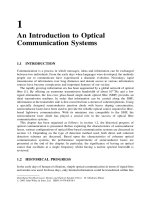
As shown in Fig. 10.3, the corrugation inside the DFB laser is assumed to extend from z ¼ z
1
to z ¼ z
2
.
The amplitude coefficients at the left and right facets can then be written as
Rz
1
ðÞ¼R
1
e
gz

1
þ S
2
e
Àj
e
Àgz
1
ð10:22aÞ
Sz
1
ðÞ¼R
1
e
j
e
gz
1
þ S
2
e
Àgz
1
ð10:22bÞ
Rz
2
ðÞ¼R
1
e
gz

2
þ S
2
e
Àj
e
Àgz
2
ð10:22cÞ
Sz
2
ðÞ¼R
1
e
j
e
gz
2
þ S
2
e
Àgz
2
ð10:22dÞ
From eqns (10.22a) and (10.22b), R
1
and S
2
can be expressed as
R

1
¼
Sz
1
ðÞe
Àj
À Rz
1
ðÞ

2
À 1ðÞe
gz
1
ð10:23aÞ
S
2
¼
Rz
1
ðÞe
j
À Sz
1
ðÞ

2
À 1ðÞe
Àgz
1

ð10:23bÞ
Subsequently, by substituting the above equations into eqns (10.22c) and (10.22d), we have
Rz
2
ðÞ¼
E À 
2
E
À1
1 À 
2
Rz
1
ðÞÀ
 E À E
À1
ÀÁ
e
Àj
1 À 
2
Sz
1
ðÞ ð10:24aÞ
Sz
2
ðÞ¼
 E À E
À1
ÀÁ

e
j
1 À 
2
Rz
1
ðÞÀ

2
E À E
À1
1 À 
2
Sz
1
ðÞ ð10:24bÞ
where
E ¼ e
g z
2
Àz
1
ðÞ
; E
À1
¼ e
Àg z
2
Àz
1

ðÞ
ð10:24cÞ
Note that the electric field at the output plane z
2
can be expressed in terms of the electric
waves at the input plane. Given the solution of the coupled wave equations from eqn (2.98)
EzðÞ¼RzðÞe
Àjb
0
z
þ SzðÞe
jb
0
z
ð10:25Þ
Figure 10.3 A simplified schematic diagram for a one-dimensional corrugated DFB laser diode
section.
SOLUTIONS OF THE COUPLED WAVE EQUATIONS
259
Equations (10.24) can then be combined with the solution of the coupled wave equations, the
output and input of the electric fields through the matrix approach can therefore be related as
E
R
z
2
ðÞ
E
S
z
2

ðÞ
!
¼ T z
2
j z
1
ðÞÁ
E
R
z
1
ðÞ
E
S
z
1
ðÞ
!
¼
t
11
t
12
t
21
t
22
!
Á
E

R
z
1
ðÞ
E
S
z
1
ðÞ
!
ð10:26Þ
where the matrix T z
2
j z
1
ðÞrepresents any wave propagation from z ¼ z
1
to z ¼ z
2
and its
elements t
ij
i; j ¼ 1; 2ðÞare given as
t
11
¼
E À 
2
E
À1

ÀÁ
Á e
Àjb
0
z
2
Àz
1
ðÞ
ð1 À 
2
Þ
ð10:27aÞ
t
12
¼
 E À E
À1
ÀÁ
Á e
Àj
e
Àjb
0
z
2
þz
1
ðÞ
ð1 À 

2
Þ
ð10:27bÞ
t
21
¼
À E À E
À1
ÀÁ
Á e
j
e
jb
0
z
2
þz
1
ðÞ
ð1 À 
2
Þ
ð10:27cÞ
t
22
¼
À 
2
E À E
À1

ÀÁ
Á e
jb
0
z
2
Àz
1
ðÞ
ð1 À 
2
Þ
ð10:27dÞ
Or from eqn (10.24) in hyperbolic functions [7]
Rz
2
ðÞ
Sz
2
ðÞ
!
¼ F z
2
j z
1
ðÞÁ
Rz
1
ðÞ
Sz

1
ðÞ
!
¼
f
11
f
12
f
21
f
22
!
Á
Rz
1
ðÞ
Sz
1
ðÞ
!
ð10:28Þ
where
f
11
¼ cosh g z
2
À z
1
ðÞ½þ

 À jðÞz
2
À z
1
ðÞ
g z
2
À z
1
ðÞ
sinh g z
2
À z
1
ðÞ½ð10:29aÞ
f
12
¼Àj
 z
2
À z
1
ðÞ
g z
2
À z
1
ðÞ
sinh g z
2

À z
1
ðÞ½ ð10:29bÞ
f
21
¼ j
 z
2
À z
1
ðÞ
 z
2
À z
1
ðÞ
sinh g z
2
À z
1
ðÞ½ ð10:29cÞ
f
22
¼ cosh g z
2
À z
1
ðÞ½À
 À jðÞz
2

À z
1
ðÞ
g z
2
À z
1
ðÞ
sinh g z
2
À z
1
ðÞ½ð10:29dÞ
Owing to conservation of energy, the determinant of the matrix T z
2
j z
1
ðÞmust always be
unity [19–20]. That is
t
11
t
22
À t
12
t
21
¼ 1 ð10:30Þ
10.3.3 Solutions of Complex Transcendental Equations using the
Newton–Raphson Approximation

Transcendental equations will be formed in order to find the threshold gain of DFB LDs
[21]. In general these equations can be expressed in complex form such that
WzðÞ¼UzðÞþjVzðÞ¼0 ð10:31Þ
260
WAVELENGTH TUNABLE OPTICAL FILTERS BASED ON DFB LASER STRUCTURES
in which the argument z ¼ x þ jy is a complex number while UzðÞand VzðÞare the real and
imaginary parts of the transcendental equations.
If WzðÞ¼0, the real and imaginary parts will subsequently be zero values. If the first-
order derivative of eqn (10.31) with respect to z is taken as
@WzðÞ
@z
¼
@UzðÞ
@z
þ j
@VzðÞ
@z
¼
@UzðÞ
@x
Á
@x
@z
þ j
@VzðÞ
@x
Á
@x
@z


¼
@UzðÞ
@x
þ j
@VzðÞ
@x
,
@x
@z
¼ 1
ð10:32Þ
By using the Taylor series, the functions UzðÞand VzðÞcan be approximated about the exact
solution x
approx
; y
approx
ÀÁ
such that
Ux
approx
; y
approx
ÀÁ
¼ Ux; yðÞþ
@U
@x
x
approx
À x
ÀÁ

þ
@U
@y
y
approx
À y
ÀÁ
ð10:33Þ
Vx
approx
; y
approx
ÀÁ
¼ Vx; yðÞþ
@V
@x
x
approx
À x
ÀÁ
þ
@V
@y
y
approx
À y
ÀÁ
ð10:34Þ
where x; yðÞis the initial guess which is chosen to be sufficiently close to the exact solutions.
The other higher-order derivative terms from the above Taylor series have been ignored.

Thus, by solving the above simultaneous equations, we have
x
approx
¼ x þ
Vx; yðÞ
@U
@y
À Ux; yðÞ
@V
@y
det
ð10:35Þ
y
approx
¼ y þ
Ux; yðÞ
@V
@x
À Vx; yðÞ
@U
@x
det
ð10:36Þ
where
det ¼
@U
@x

2
þ

@V
@y

2
ð10:37Þ
For an analytical complex function WzðÞ, the Cauchy–Riemann condition must be satisfied [22]
@U
@x
¼
@V
@y
;
@U
@y
¼À
@V
@x
ð10:38Þ
The partial differential with respect to y, @=@y will then be replaced with @=@x using the
above Cauchy–Riemann condition
det ¼ 2
@U
@x

2
ð10:39Þ
x
approx
¼ x À
Vx; yðÞ

@V
@x
þ Ux; yðÞ
@U
@x
det
ð10:40Þ
Only the first-order derivatives @U=@x and @V=@x are used to solve eqn (10.32).
SOLUTIONS OF THE COUPLED WAVE EQUATIONS
261
Initially, a pair x; yðÞis guessed in order to start the numerical iteration process. A new
pair x
approx
; y
approx
ÀÁ
is then generated until it is sufficiently close to the exact solution.
Though there are many other numerical methods to solve transcendental equations, this
method is used due to its flexibility and speed. In addition, any errors associated with other
numerical methods, such as numerical differentiation, can be avoided. However, the
derivative term @W=@z must be solved analytically before any numerical iteration is
undertaken. Another numerical method in which the term @W=@z cannot be solved
analytically for the case of tapered-structure DFB LDs shall now be discussed.
10.4 THRESHOLD ANALYSIS OF DFB LASER DIODES
For a conventional DFB laser with a zero facet reflection, the threshold eigenvalue
eqn (10.16) becomes
jgL ¼ÆL sinh gLðÞ ð10:41Þ
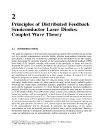
The above transcendental equation is then solved using the Newton–Raphson iteration
approach in which the coupling coefficient is given. The results obtained are shown in
Fig. 10.4.

Figure 10.4 The normalised amplitude gain versus the normalised detuning coefficient of a uniform
index-coupled DFB LD.
262
WAVELENGTH TUNABLE OPTICAL FILTERS BASED ON DFB LASER STRUCTURES
Note that all parameters used have been normalised with respect to the overall cavity
length L. Different values of normalised coupling coefficient L in the range 0.25 to 5.0 have
been set. As predicted mathematically, there exist two pairs of possible solutions for each
oscillation mode (complex conjugates). Thus, from the results, we can see that the
oscillating modes distribute symmetrically with respect to the Bragg wavelength, where
L ¼ 0. In addition, no oscillation can be found at the Bragg wavelength. This region
between the þ1 and À1 modes is called the stop band as discussed in section 10.3.1. From
Fig. 10.4, it can also be seen that when the coupling strength increases, the normalised
amplitude gain will decrease, in other words, the threshold current will be decreasing. This is
because a larger value of L indicates a stronger optical feedback along the DFB cavity.
Similarly, if the coupling strength is fixed, a longer cavity length will also reduce the
threshold gains since a larger single pass gain can be achieved easily.
In laser operation, the main (fundamental) mode is large and the sub-modes are
sufficiently suppressed because the coupling between the main mode and the sub-modes is
large and, as such, the gain concentrates on the main mode. However, if DFB LDs are to be
used as amplifier filters, the lasers will then be biased below the lasing threshold, therefore
the gain difference between the main mode and the sub-modes is always smaller than in laser
operation. As a result, the wavelength tuning range for an optical amplifier filter is smaller
than that of a laser.
10.4.1 Phase Discontinuities in DFB LDs
The analysis of phase-adjusted DFB LDs is rather similar to the conventional DFB LDs
described in the previous section. The only difference is that the boundary conditions at the
phase shift position (PSP) have to be matched. Whenever a propagating wave travels past a
phase discontinuity along the corrugation, it will experience a phase delay.
As noted earlier, TMM is used since it can match the boundary conditions easily by
cascading the matrices. Thus, the phase discontinuity along the cavity of the DFB LDs can

be best explained by using a two-section DFB structure with a single phase shift at the centre
of the corrugation as depicted in Fig. 10.5. z
þ

and z
À

are assumed to be the slight deviations
from z

.
Figure 10.5 Schematic diagram of a single-phase-shifted DFB LD.
THRESHOLD ANALYSIS OF DFB LASER DIODES
263
If the distance between z

and z
Æ

is infinitesimal, we can relate the electric fields at z
þ

and
z
À

as follows
E
R
z

þ

ÀÁ
E
S
z
þ

ÀÁ
"#
¼
e
j
0
0e
Àj
"#
Á
E
R
z
À

ÀÁ
E
S
z
À

ÀÁ

"#
¼ P

Á
E
R
z
À

ÀÁ
E
S
z
À

ÀÁ
"#
ð10:42Þ
where P

is the phase discontinuity matrix, which causes the complex electric field delay
of  at z ¼ z

. By applying the phase discontinuity to eqn (10.26) and following the steps
below it,
E
R
z
À


ÀÁ
E
S
z
À

ÀÁ
"#
¼ T
1
Á
E
R
z
1
ðÞ
E
S
z
1
ðÞ
!
ð10:43Þ
where T
1
is the transfer matrix defined in eqns (10.27a) – (10.27d).
E
R
z
þ


ÀÁ
E
S
z
þ

ÀÁ
"#
¼ P

Á
E
R
z
À

ÀÁ
E
S
z
À

ÀÁ
"#
ð10:44Þ
E
R
z
2

ðÞ
E
S
z
2
ðÞ
!
¼ T
2
Á
E
R
z
þ

ÀÁ
E
S
z
þ

ÀÁ
"#
ð10:45Þ
If the above concept is employed for N-section (N ! 1) multiple-phase-shifted (MPS) DFB
LDs, the general TMM equation can be expressed as
E
R
z
Nþ1

ðÞ
E
S
z
Nþ1
ðÞ
!
¼ T
N
P

T
NÀ1
P

...T
1
Á
E
R
z
1
ðÞ
E
S
z
1
ðÞ
!
¼

Y
k¼N
k¼1
T
k
P

Á
E
R
z
1
ðÞ
E
S
z
1
ðÞ
!
ð10:46Þ
Thus far, various numbers of phase discontinuities are being proposed [23–25].
These include the novel multiple-phase-shift DFB LD proposed by Tan et al. and shown
in Fig. 10.6 [25].
Figure 10.6 Analytical model for a 3-phase-shift DFB LD structure [25].
264
WAVELENGTH TUNABLE OPTICAL FILTERS BASED ON DFB LASER STRUCTURES