Tài liệu Multisensor thiết bị đo đạc thiết kế 6o (P1) docx

1
1
PROCESS, QUANTUM, AND
ANALYTICAL SENSORS
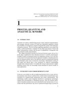
1-0 INTRODUCTION
Automatic test systems, manufacturing process control, analytical instrumentation,
and aerospace electronic systems all would have diminished capabilities without
the availability of contemporary computer integrated data systems with multisensor
information structures. This text develops supporting quantitative error models that
enable a unified performance evaluation for the design and analysis of linear and
digital instrumentation systems with the goal of compatibility of integration with
other enterprise quality representations.
This chapter specifically describes the front-end electrical sensor devices for a
broad range of applications from industrial processes to scientific measurements.
Examples include environmental sensors for temperature, pressure, level, and flow;
in situ sensors for measurements beyond apparatus boundaries, including spectrom-
eters for chemical analysis; and ex situ analytical sensors for manufactured material
and biomedical assays such as microwave microscopy. Hyperspectral sensing of
both spatial and spectral data is also introduced for improved understanding
through feature characterization. It is notable that owing to advancements in higher
attribution sensors, they are increasingly being substituted for process models in
many applications.
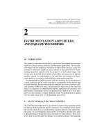
1-1 INSTRUMENTATION ERROR REPRESENTATION
In this text, error models are derived employing electronic device, circuit, and sys-
tem parameter values that are combined into a unified end-to-end performance rep-
resentation for computer-based measurement and control instrumentation. This
methodology enables system integration beneficial to contemporary technologies
ranging from micromachines to distributed processes. Since the baseline perfor-
mance of machines and processes can be described by their internal errors, it is ax-
iomatic that their performance may also be optimized through design in pursuit of
Multisensor Instrumentation 6

␴
Design. By Patrick H. Garrett
Copyright © 2002 by John Wiley & Sons, Inc.
ISBNs: 0-471-20506-0 (Print); 0-471-22155-4 (Electronic)
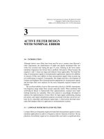
error minimization. Instrumentation system errors are interpreted graphically in
Figure 1-1. Total error is shown as the composite of barred mean error contributions
plus the root-sum-square (RSS) of systematic and random uncertainties; the true
value is ultimately traceable to a reference calibration standard harbored by NIST.
Although total error may instantaneously be greater or less than mean error from
the additivity of RSS uncertainty error, throughout this text total error is expressed
as the sum of mean and RSS errors in providing accountability of system behavior.
Total error is analytically expressed by equation (1-1) as 0–100% of full scale
(%FS), where the RSS sum of variances represents a one-sigma confidence interval.
Consequently, total error may be expressed over any confidence interval by adding
one mean error value and a summation of RSS error values corresponding to the stan-
dard deviation integer. Confidence to six sigma is therefore defined by mean error
plus six times the RSS error value. Mean error frequently arises in instrumentation
systems from transfer function nonlinearities that, unlike RSS uncertainty error,
which may be reduced by averaging identical systems as shown in Chapter 4, Section
4-4, instead increases with the addition of each mean error contribution, necessitat-
ing remedy through minimal inclusion. Accuracy is defined as the complement of er-
ror (100%FS – ␧%FS), where 1%FS error corresponds to 99%FS accuracy.
A six-sigma framework is accordingly offered in terms of models defining mul-
tisensor instrumentation errors to provide a generic design and analysis methodolo-
gy compatible with corollary enterprise-quality representations. Quantitative instru-
mentation system performance expressed in terms of modeled errors assumes that
external calibration is maintained to known standards, as shown in Figure 1-21, ver-
ifying zero and full-scale values for external instrumentation registration. Calibra-
tion is essential and can be performed manually or by automated methods, but it
cannot characterize instrumentation device, circuit, and system variabilities that

these error budgets ably describe, including expression to 6␴ confidence.
␧
total
= ⌺ ␧
ෆ
m
ෆ
e
ෆ
a
ෆ
n
ෆ
%FS + [⌺ ␧
2
systematic
+ ⌺ ␧
2
random
]
1/2
%FS1␴ (1-1)
2
PROCESS, QUANTUM, AND ANALYTICAL SENSORS
FIGURE 1-1. Instrumentation error interpretation.
Figure 1-2 describes generic measurement elements, where the sensor represents
a physical device employed at a measurement interface, and the transducer princi-
ple the translation involved between measurand units and a corresponding signal
representation. For example, in the application of a thermocouple, the physical con-
tact of two dissimilar alloys with a thermal process constitutes the sensor, but the

emf signal arising at discrete temperature values is attributable to the Seebeck trans-
ducer effect. Many sensors, such as strain-gauge bridges, further require external
excitation to generate a measurement signal as well as a specific interface circuit.
Seven measurement definitions follow:
Accuracy: the closeness with which a measurement approaches the true value
of a measurand, usually expressed as a percent of full scale
Error: the deviation of a measurement from the true value of a measur-
and, usually expressed as a percent of full scale
Tolerance: allowable error deviation about a reference of interest
Precision: an expression of a measurement over some span described by the
number of significant figures available
Resolution: an expression of the smallest quantity to which a quantity can be
represented
Span: an expression of the extent of a measurement between any two
limits
Range: an expression of the total extent of measurement values
Technology has advanced significantly as a consequence of sensor development.
However, measurement is an inexact discipline requiring the use of reference stan-
dards to provide accountability for sensor signals with respect to their measurands.
Fortunately, sensor nonlinearity can be minimized by means of multipoint calibra-
tion. Practical implementation often requires the synthesis of a linearized output
function that achieves the best asymptotic approximation to the true value over a
sensor measurement range of interest. The resulting straight-line fit is often realized
after digital signal conversion to benefit from the accuracy of digital computation.
The cubic function of equation (1-2) is an effective linearizing equation demon-
strated over the full 700°C range of a commonly applied Type-J thermocouple,
which is tabulated in Table 1-1. Solution of the A and B coefficients at judiciously
spaced temperature values defines the linearizing equation with a 0°C intercept.
Evaluation at linearized 100°C intervals throughout the thermocouple range reveals
1-1 INSTRUMENTATION ERROR REPRESENTATION

3
FIGURE 1-2. Generic sensor elements.
temperature values nominally within 1°C of their true temperatures, which corre-
spond to typical errors of 0.25%FS. It is also useful to express the average of dis-
crete errors over the sensor range, obtaining a mean error value of 0
ෆ
.
ෆ
1
ෆ
1
ෆ
%FS for the
Type-J thermocouple. This example illustrates a design goal proffered throughout
this text of not exceeding one-tenth percent error for any contributing system ele-
ment. Extended polynomials permit further reduction in linearized sensor error
while incurring increased computational burden, where a fifth-order equation can
beneficially provide linearization to 0.1°C, corresponding to 0
ෆ
.
ෆ
0
ෆ
1
ෆ
%FS mean error.
y = AX + BX
3
+ intercept (1-2)
Coefficient for 10.779 mV at 200°C:

200°C = A(10.779 mV) + B(10.779mV)
3
+ 0°C
A = 18.5546 – B(116.186mV
2
)
Coefficient for 27.393 mV at 500°C:
500°C = 508.2662 °C – B(3182.68 mV
3
) + B(20,555.0 mV
3
)
A = 18.6099 B = –0.000475
1-2 TEMPERATURE SENSORS
Thermocouples are widely used as temperature sensors because of their ruggedness
and broad temperature range. Two dissimilar metals are used in the Seebeck effect
°C
ᎏ
mV
3
°C
ᎏ
mV
4
PROCESS, QUANTUM, AND ANALYTICAL SENSORS
TABLE 1-1. Sensor Cubic Linearization
Y °C X mV y °C ␧
%FS
= |(Y – y)100%/700°C|
00 0 0

100 5.269 98 0.27
200 10.779 200 0
300 16.327 302 0.25
400 21.848 401 0.23
500 27.393 500 0
600 33.102 599 0.17
700 39.132 700 0
Y true temperature 0
ෆ
.
ෆ
1
ෆ
1
ෆ
%FS mean error
X Type-J thermocouple signal 0°C intercept
y linearized temperature 700°C full scale
temperature-to-emf junction with transfer relationships described by Figure 1-3.
Proper operation requires the use of a thermocouple reference junction in series
with the measurement junction to polarize the direction of current flow and maxi-
mize the measurement emf. Omission of the reference junction introduces an uncer-
tainty evident as a lack of measurement repeatability equal to the ambient tempera-
ture.
An electronic reference junction that does not require an isolated supply can be
realized with an Analog Devices AD590 temperature sensor, as shown in Figure 4-
5. This reference junction usually is attached to an input terminal barrier strip in or-
der to track the thermocouple-to-copper circuit connection thermally. The error sig-
nal is referenced to the Seebeck coefficients in mV/°C (see Table 1-2) and provided
as a compensation signal for ambient temperature variation. The single calibration

trim at ambient temperature provides temperature tracking within a few tenths of a
°C.
Resistance thermometer devices (RTDs) provide greater resolution and repeata-
bility than thermocouples, the latter typically being limited to approximately 1 °C.
RTDs operate on the principle of resistance change as a function of temperature,
and are represented by a number of devices. The platinum resistance thermometer is
frequently utilized in industrial applications because it offers good accuracy with
mechanical and electrical stability. Thermistors are fabricated by sintering a mix-
ture of metal alloys to form a ceramic that exhibits a significant negative tempera-
ture coefficient. Metal film resistors have an extended and more linear range than
thermistors, but thermistors exhibit approximately ten times their sensitivity. RTDs
require excitation, usually provided as a constant current source, in order to convert
1-2 TEMPERATURE SENSORS
5
FIGURE 1-3. Temperature–millivolt graph for thermocouples. (Courtesy of Omega Engi-
neering, Inc., an Omega Group Company.)
their resistance change with temperature into a voltage change. Figure 1-4 presents
the temperature–resistance characteristics of common RTD sensors.
Optical pyrometers are utilized for temperature measurement when sensor phys-
ical contact with a process is not feasible but a view is available. Measurements are
limited to energy emissions within the spectral response capability of the specific
sensor used. A radiometric match of emissions between a calibrated reference
source and the source of interest provides a current analog corresponding to temper-
ature. Automatic pyrometers employ a servo loop to achieve this balance, as shown
in Figure 1-5. Operation to 5000°C is available.
6
PROCESS, QUANTUM, AND ANALYTICAL SENSORS
TABLE 1-2. Thermocouple Comparison Data
Type Elements, +/– mV/°C Range (°C) Application
E Chromel/constantan 0.063 0 to 800 High output

J Iron/constantan 0.054 0 to 700 Reducing atmospheres
K Chromel/alumel 0.040 0 to 1,200 Oxidizing atmospheres
R&S Pt-Rb/platinum 0.010 0 to 1,400 Corrosive atmospheres
T Copper/constantan 0.040 –250 to 350 Moist atmospheres
C Tungsten/rhenium 0.012 0 to 2,000 High temperature
FIGURE 1-4. RTD devices.
1-3 MECHANICAL SENSORS
Fluid pressure is defined as the force per unit exerted by a gas or a liquid on the
boundaries of a containment vessel. Pressure is a measure of the energy content of
hydraulic and pneumatic (liquid and gas) fluids. Hydrostatic pressure refers to the
internal pressure at any point within a liquid directly proportional to the liquid
height above that point, independent of vessel shape. The static pressure of a gas
refers to its potential for doing work, which does not vary uniformly with height as
a consequence of its compressibility. Equation (1-3) expresses the basic relation-
ship between pressure, volume, and temperature as the general gas law. Pressure
typically is expressed in terms of pounds per square inch (psi) or inches of water (in
H
2
O) or mercury (in Hg). Absolute pressure measurements are referenced to a
vacuum, whereas gauge pressure measurements are referenced to the atmosphere.
= Constant (1-3)
A pressure sensor detects pressure and provides a proportional analog signal by
means of a pressure–force summing device. This usually is implemented with a me-
chanical diaphragm and linkage to an electrical element such as a potentiometer,
strain gauge, or piezoresistor. Quantities of interest associated with pressure–force
summing sensors include their mass, spring constant, and natural frequency.
Potentiometric elements are low in cost and have high output, but their sensitivity to
vibration and mechanical nonlinearities combine to limit their utility. Unbonded
strain gauges offer improvement in accuracy and stability, with errors to 0.5% of full
scale, but their low output signal requires a preamplifier. Present developments in

Absolute temperature × Gas volume
ᎏᎏᎏᎏ
Absolute pressure
1-3 MECHANICAL SENSORS
7
FIGURE 1-5. Automatic pyrometer.
pressure transducers involve integral techniques to compensate for the various error
sources, including crystal diaphragms for freedom from measurement hysteresis.
Figure 1-6 illustrates a microsensor circuit pressure transducer for enhanced reliabil-
ity with an internal vacuum reference, chip heating to minimize temperature errors,
and a piezoresistor bridge transducer circuit with on-chip signal conditioning.
Liquid levels are frequently required to process measurements in tanks, pipes,
and other vessels. Sensing methods of various complexity are employed, including
float devices, differential pressure, ultrasonics, and bubblers. Float devices offer
simplicity and various ways of translating motion into a level reading. A differential
pressure transducer can also measure the height of a liquid when its specific weight
W is known, and a ⌬P cell is connected between the vessel surface and bottom.
Height is provided by the ratio of ⌬P/W.
Accurate sensing of position, shaft angle, and linear displacement is possible
with the linear variable displacement transformer (LVDT). With this device, an ac
excitation introduced through a variable reluctance circuit is induced in an output
circuit through a movable core that determines the amount of displacement. LVDT
advantages include overload capability and temperature insensitivity. Sensitivity in-
creases with excitation frequency, but a minimum ratio of 10:1 between excitation
and signal frequencies is considered a practical limit. LVDT variants include the in-
duction potentiometer, synchros, resolvers, and the microsyn. Figure 1-7 describes
a basic LVDT circuit with both ac and dc outputs.
Fluid flow measurement generally is implemented either by differential pres-
sure or mechanical contact sensing. Flow rate F is the time rate of fluid motion
with dimensions typically in feet per second. Volumetric flow Q is the fluid vol-

ume per unit time, such as gallons per minute. Mass flow rate M for a gas is de-
fined, for example, in terms of pounds per second. Differential pressure flow sens-
ing elements are also known as variable head meters because the pressure
difference between the two measurements ⌬P is equal to the head. This is equiv-
8
PROCESS, QUANTUM, AND ANALYTICAL SENSORS
FIGURE 1-6. Integrated pressure microsensor.
alent to the height of the column of a differential manometer. Flow rate is there-
fore obtained with the 32 ft/sec
2
gravitational constant g and differential pressure
by equation (1-4). Liquid flow in open channels is obtained by head-producing de-
vices such as flumes and weirs. Volumetric flow is obtained with the flow cross-
sectional area and the height of the flow over a weir, as shown by Figure 1-8 and
equation (1-5).
Flow rate F =
͙
2
ෆ
g
ෆ
⌬
ෆ
P
ෆ
feet/second (1-4)
Volumetric flow Q =
͙
2
ෆ

g
ෆ
L
ෆ
2
H
ෆ
3
ෆ
cubic feet/second (1-5)
Mass flow M =
Ί
R
๶
๶
·
Ί
๶
pounds/second (1-6)
where
R = universal gas constant
⌬P
0
= true differential pressure, P
0
– P
ϱ
⌬P
x
= calibration differential pressure

Acceleration measurements are principally of interest for shock and vibration
sensing. Potentiometric dashpots and capacitive transducers have largely been sup-
planted by piezoelectric crystals. Their equivalent circuit is a voltage source in se-
ries with a capacitance, as shown in Figure 1-9 which produces an output in
P⌬P
ᎏ
T
⌬P
0
ᎏ
⌬P
x
1-3 MECHANICAL SENSORS
9
FIGURE 1-7. Basic LVDT.