Tài liệu Multisensor thiết bị đo đạc thiết kế 6o (P3) doc

47
3
ACTIVE FILTER DESIGN
WITH NOMINAL ERROR
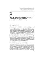
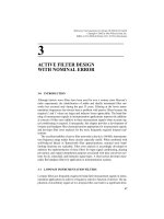
3-0 INTRODUCTION
Although electric wave filters have been used for over a century since Marconi’s
radio experiments, the identification of stable and ideally terminated filter net-
works has occurred only during the past 35 years. Filtering at the lower instru-
mentation frequencies has always been a problem with passive filters because the
required L and C values are larger and inductor losses appreciable. The band-lim-
iting of measurement signals in instrumentation applications imposes the addition-
al concern of filter error additive to these measurement signals when accurate sig-
nal conditioning is required. Consequently, this chapter provides a development of
lowpass and bandpass filter characterizations appropriate for measurement signals,
and develops filter error analyses for the more frequently required lowpass real-
izations.
The excellent stability of active filter networks in the dc to 100 kHz instrumenta-
tion frequency range makes these circuits especially useful. When combined with
well-behaved Bessel or Butterworth filter approximations, nominal error band-
limiting functions are realizable. Filter error analysis is accordingly developed to
optimize the implementation of these filters for input signal conditioning, aliasing
prevention, and output interpolation purposes associated with data conversion sys-
tems for dc, sinusoidal, and harmonic signal types. A final section develops maxi-
mally flat bandpass filters for application in instrumentation systems.
3-1 LOWPASS INSTRUMENTATION FILTERS
Lowpass filters are frequently required to band-limit measurement signals in instru-
mentation applications to achieve a frequency-selective function of interest. The ap-
plication of an arbitrary signal set to a lowpass filter can result in a significant atten-
Multisensor Instrumentation 6
␴
Design. By Patrick H. Garrett

Copyright © 2002 by John Wiley & Sons, Inc.
ISBNs: 0-471-20506-0 (Print); 0-471-22155-4 (Electronic)
uation of higher frequency components, thereby defining a stopband whose bound-
ary is influenced by the choice of filter cutoff frequency, with the unattenuated fre-
quency components defining the filter passband. For instrumentation purposes, ap-
proximating the ideal lowpass filter amplitude A( f ) and phase B( f ) responses
described by Figure 3-1 is beneficial in order to achieve signal band-limiting with-
out alteration or the addition of errors to a passband signal of interest. In fact, pre-
serving the accuracy of measurement signals is of sufficient importance that consid-
eration of filter characterizations that correspond to well-behaved functions such as
Butterworth and Bessel polynomials are especially useful. However, an ideal filter
is physically unrealizable because practical filters are represented by ratios of poly-
nomials that cannot possess the discontinuities required for sharply defined filter
boundaries.
Figure 3-2 describes the Butterworth lowpass amplitude response A( f ) and Fig-
ure 3-3 its phase response B( f ), where n denotes the filter order or number of poles.
Butterworth filters are characterized by a maximally flat amplitude response in the
vicinity of dc, which extends toward its –3 dB cutoff frequency f
c
as n increases.
This characteristic is defined by equations (3-1) and (3-2) and Table 3-1. Butter-
worth attenuation is rapid beyond f
c
as filter order increases with a slightly nonlin-
ear phase response that provides a good approximation to an ideal lowpass filter.
An analysis of the error attributable to this approximation is derived in Section 3-3.
Figure 3-4 presents the Butterworth highpass response.
B(s) =
΂
j

΃
n
+ b
n–1
΂
j
΃
n–1
+ ··· + b
0
(3-1)
f
ᎏ
f
c
f
ᎏ
f
c
48
ACTIVE FILTER DESIGN WITH NOMINAL ERROR
FIGURE 3-1. Ideal lowpass filter.
3-1 LOWPASS INSTRUMENTATION FILTERS
49
FIGURE 3-2. Butterworth lowpass amplitude.
FIGURE 3-3. Butterworth lowpass phase.
A( f ) = (3-2)
=
Bessel filters are all-pole filters, like their Butterworth counterparts. with an
amplitude response described by equations (3-3) and (3-4) and Table 3-2. Bessel

lowpass filters are characterized by a more linear phase delay extending to their
cutoff frequency f
c
and beyond as a function of filter order n shown in Figure
3-5. However, this linear-phase property applies only to lowpass filters. Unlike the
1
ᎏᎏ
͙
1
ෆ
+
ෆ
(
ෆ
f/
ෆ
f
c
ෆ
)
2
ෆ
n
ෆ
b
0
ᎏᎏ
͙
B
ෆ

(s
ෆ
)B
ෆ
(–
ෆ
s)
ෆ
50
ACTIVE FILTER DESIGN WITH NOMINAL ERROR
FIGURE 3-4. Butterworth highpass amplitude.
TABLE 3-1. Butterworth Polynomial Coefficients
Poles nb
0
b
1
b
2
b
3
b
4
b
5
11.0
2 1.0 1.414
3 1.0 2.0 2.0
4 1.0 2.613 3.414 2.613
5 1.0 3.236 5.236 5.236 3.236
6 1.0 3.864 7.464 9.141 7.464 3.864

flat passband of Butterworth lowpass filters, the Bessel passband has no value that
does not exhibit amplitude attenuation with a Gaussian amplitude response de-
scribed by Figure 3-6. It is also useful to compare the overshoot of Bessel and
Butterworth filters in Table 3-3, which reveals the Bessel to be much better be-
haved for bandlimiting pulse-type instrumentation signals and where phase linear-
ity is essential.
A( f ) = (3-3)
B(s) =
΂
j
΃
n
+ b
n–1
΂
j
΃
n–1
+ · · · + b
0
(3-4)
f
ᎏ
f
c
f
ᎏ
f
c
b

0
ᎏᎏ
͙
B
ෆ
(s
ෆ
)B
ෆ
(–
ෆ
s)
ෆ
3-1 LOWPASS INSTRUMENTATION FILTERS
51
TABLE 3-2. Bessel Polynomial Coefficients
Poles nb
0
b
1
b
2
b
3
b
4
b
5
11
233

31515 6
4 105 105 45 10
5 945 945 420 105 15
6 10,395 10,395 4725 1260 210 21
FIGURE 3-5. Bessel lowpass phase.
3-2 ACTIVE FILTER NETWORKS
In 1955, Sallen and Key of MIT published a description of 18 active filter networks
for the realization of various filter approximations. However, a rigorous sensitivity
analysis by Geffe and others disclosed by 1967 that only four of the original net-
works exhibited low sensitivity to component drift. Of these, the unity-gain and
multiple-feedback networks are of particular value for implementing lowpass and
bandpass filters, respectively, to Q values of 10. Work by others resulted in the low-
sensitivity biquad resonator, which can provide stable Q values to 200, and the sta-
ble gyrator band-reject filter. These four networks are shown in Figure 3-7 with key
sensitivity parameters. The sensitivity of a network can be determined, for example,
when the change in its Q for a change in its passive-element values is evaluated.
Equation (3-5) describes the change in the Q of a network by multiplying the ther-
mal coefficient of the component of interest by its sensitivity coefficient. Normally,
50 to 100 ppm/°C components yield good performance.
52
ACTIVE FILTER DESIGN WITH NOMINAL ERROR
FIGURE 3-6. Bessel lowpass amplitude.
TABLE 3-3. Filter Overshoot Pulse Response
n Bessel (%FS) Butterworth (%FS)
10 0
20.4 4
30.7 8
4 0.8 11
3-2 ACTIVE FILTER NETWORKS
53

FIGURE 3-7. Recommended active filter networks: (a) unity gain, (b) multiple feedback,
(c) biquad, and (d) gyrator.
S
z
Q
= ±1 passive network (3-5)
= (±1)(50 ppm/°C)(100%)
= ±0.005%Q/°C
Unity-gain networks offer excellent performance for lowpass and highpass real-
izations and may be cascaded for higher-order filters. This is perhaps the most
widely applied active filter circuit. Note that its sensitivity coefficients are less than
unity for its passive components—the sensitivity of conventional passive net-
works—and that its resistor temperature coefficients are zero. However, it is sensi-
tive to filter gain, indicating that designs that also obtain greater than unity gain
with this filter network are suboptimum. The advantage of the multiple-feedback
network is that a bandpass filter can be formed with a single operational amplifier,
although the biquad network must be used for high Q bandpass filters. However,
the stability of the biquad at higher Q values depends upon the availability of ade-
quate amplifier loop gain at the filter center frequency. Both bandpass networks can
be stagger-tuned for a maximally flat passband response when required. The princi-
ple of operation of the gyrator is that a conductance –G gyrates a capacitive current
to an effective inductive current. Frequency stability is very good, and a band-reject
filter notch depth to about –40 dB is generally available. It should be appreciated
that the principal capability of the active filter network is to synthesize a com-
plex–conjugate pole pair. This achievement, as described below, permits the real-
ization of any mathematically definable filter approximation.
Kirchoff’s current law provides that the sum of the currents into any node is
zero. A nodal analysis of the unity-gain lowpass network yields equations (3-6)
through (3-9). It includes the assumption that current in C
2

is equal to current in R
2
;
the realization of this requires the use of a low-input-bias-current operational ampli-
fier for accurate performance. The transfer function is obtained upon substituting
for V
x
in equation (3-6) its independent expression obtained from equation (3-7).
Filter pole positions are defined by equation (3-9). Figure 3-8 shows these nodal
equations and the complex-plane pole positions mathematically described by equa-
tion (3-9). This second-order network has two denominator roots (two poles) and is
sometimes referred to as a resonator.
= + (3-6)
= (3-7)
Rearranging,
V
x
= V
0
·
= (3-8)
1
ᎏᎏᎏᎏ
␻
2
R
1
R
2
C

1
C
2
+
␻
C
2
(R
1
+ R
2
) + 1
V
0
ᎏ
V
i
R
2
+ 1/j
␻
C
2
ᎏᎏ
1/j
␻
C
2
V
0

ᎏ
1/j
␻
C
2
V
x
– V
0
ᎏ
R
2
V
x
– V
0
ᎏ
R
2
V
x
– V
0
ᎏ
1/j
␻
C
1
V
i

– V
x
ᎏ
R
1
54
ACTIVE FILTER DESIGN WITH NOMINAL ERROR
␻
1
= and
␻
2
= and
␦
= (R
1
+ R
2
)
s
1,2
= –
␦
͙
␻
ෆ
1
␻
ෆ
2

ෆ
± j
͙
␻
ෆ
1
␻
ෆ
2
ෆ
·
͙
1
ෆ
–
ෆ
␦
ෆ
2
ෆ
(3-9)
A recent technique using MOS technology has made possible the realization of
multipole unity-gain network active filters in total integrated circuit form without
the requirement for external components. Small-value MOS capacitors are utilized
with MOS switches in a switched-capacitor circuit for simulating large-value re-
sistors under control of a multiphase clock. With reference to Figure 3-9 the rate
f
s
at which the capacitor is toggled determines its charging to V and discharging to
VЈ. Consequently, the average current flow I from V to VЈ defines an equivalent

resistor R that would provide the same average current shown by the identity of
C
2
ᎏ
2
1
ᎏ
R
2
C
2
1
ᎏ
R
1
C
1
3-2 ACTIVE FILTER NETWORKS
55
FIGURE 3-8. Unity-gain network nodal analysis.
equation (3-10). The switching rate f
s
is normally much higher than the signal fre-
quencies of interest so that the time sampling of the signal can be ignored in a
simplified analysis. Filter accuracy is primarily determined by the stability of the
frequency of f
s
and the accuracy of implementation of the monolithic MOS ca-
pacitor ratios.
R = = 1/Cf

c
(3-10)
The most important parameter in the selection of operational amplifiers for ac-
tive filter service is open-loop gain. The ratio of open-loop to closed-loop gain, or
loop gain, must be 10
2
or greater for stable and well-behaved performance at the
highest signal frequencies present. This is critical in the application of bandpass fil-
ters to ensure a realization that accurately follows the design calculations. Amplifi-
er input and output impedances are normally sufficiently close to the ideal infinite
input and zero output values to be inconsequential for impedances in active filter
networks. Metal film resistors having a temperature coefficient of 50 ppm/°C are
recommended for active filter design.
Selection of capacitor type is the most difficult decision because of many inter-
acting factors. For most applications, polystyrene capacitors are recommended be-
cause of their reliable –120 ppm/°C temperature coefficient and 0.05% capacitance
retrace deviation with temperature cycling. Where capacitance values above 0.1 ␮F
are required, however, polycarbonate capacitors are available in values to 1 ␮F with
a ±50 ppm/°C temperature coefficient and 0.25% retrace. Mica capacitors are the
V – VЈ
ᎏ
I
56
ACTIVE FILTER DESIGN WITH NOMINAL ERROR
FIGURE 3-9. Switched capacitor unity-gain network.
most stable devices with ± 50 ppm/°C tempco and 0.1% retrace, but practical ca-
pacitance availability is typically only 100 pF to 5000 pF. Mylar capacitors are
available in values to 10 ␮F with 0.3% retrace, but their tempco averages 400
ppm/°C.
The choice of resistor and capacitor tolerance determines the accuracy of the

filter implementation such as its cutoff frequency and passband flatness. Cost con-
siderations normally dictate the choice of 1% tolerance resistors and 2–5% toler-
ance capacitors. However, it is usual practice to pair larger and smaller capacitor
values to achieve required filter network values to within 1%, which results in fil-
ter parameters accurate to 1 or 2% with low tempco and retrace components.
Filter response is typically displaced inversely to passive-component tolerance,
such as lowering of cutoff frequency for component values on the high side of
their tolerance band. For more critical realizations, such as high-Q bandpass fil-
ters, some provision for adjustment provides flexibility needed for an accurate im-
plementation.
Table 3-4 provides the capacitor values in farads for unity-gain networks tabulat-
ed according to the number of filter poles. Higher-order filters are formed by a cas-
cade of the second- and third-order networks shown in Figure 3-10, each of which
is different. For example, a sixth-order filter will have six different capacitor values
and not consist of a cascade of identical two-pole or three-pole networks. Figures
3-11 and 3-12 illustrate the design procedure with 1 kHz cutoff, two-pole Butter-
worth lowpass and highpass filters including the frequency and impedance scaling
steps. The three-pole filter design procedure is identical with observation of the ap-
3-2 ACTIVE FILTER NETWORKS
57
TABLE 3-4. Unity-Gain Network Capacitor Values in Farads
Butterworth Bessel
______________________________ _____________________________
Poles C
1
C
2
C
3
C

1
C
2
C
3
2 1.414 0.707 0.907 0.680
3 3.546 1.392 0.202 1.423 0.988 0.254
4 1.082 0.924 0.735 0.675
2.613 0.383 1.012 0.390
5 1.753 1.354 0.421 1.009 0.871 0.309
3.235 0.309 1.041 0.310
6 1.035 0.966 0.635 0.610
1.414 0.707 0.723 0.484
3.863 0.259 1.073 0.256
7 1.531 1.336 0.488 0.853 0.779 0.303
1.604 0.624 0.725 0.415
4.493 0.223 1.098 0.216
8 1.091 0.981 0.567 0.554
1.202 0.831 0.609 0.486
1.800 0.556 0.726 0.359
5.125 0.195 1.116 0.186