Tài liệu Multisensor thiết bị đo đạc thiết kế 6o (P4) pptx

75
4
LINEAR SIGNAL CONDITIONING TO
SIX-SIGMA CONFIDENCE
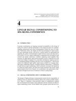
4-0 INTRODUCTION
Economic considerations are imposing increased accountability on the design of
analog I/O systems to provide performance at the required accuracy for computer-
integrated measurement and control instrumentation without the costs of overde-
sign. Within that context, this chapter provides the development of signal acquisi-
tion and conditioning circuits, and derives a unified method for representing and
upgrading the quality of instrumentation signals between sensors and data-conver-
sion systems. Low-level signal conditioning is comprehensively developed for both
coherent and random interference conditions employing sensor–amplifier–filter
structures for signal quality improvement presented in terms of detailed device and
system error budgets. Examples for dc, sinusoidal, and harmonic signals are provid-
ed, including grounding, shielding, and noise circuit considerations. A final section
explores the additional signal quality improvement available by averaging redun-
dant signal conditioning channels, including reliability enhancement. A distinction
is made between signal conditioning, which is primarily concerned with operations
for improving signal quality, and signal processing operations that assume signal
quality already at the level of interest. An overall theme is the optimization of per-
formance through the provision of methods for effective analog design.
4-1 SIGNAL CONDITIONING INPUT CONSIDERATIONS
The designer of high-performance instrumentation systems has the responsibility of
defining criteria for determining preferred options from among available alterna-
tives. Figure 4-1 illustrates a cause-and-effect outline of comprehensive methods
that are developed in this chapter, whose application aids the realization of effective
signal conditioning circuits. In this fishbone chart, grouped system and device op-
Multisensor Instrumentation 6
␴
Design. By Patrick H. Garrett

Copyright © 2002 by John Wiley & Sons, Inc.
ISBNs: 0-471-20506-0 (Print); 0-471-22155-4 (Electronic)
tions are outlined for contributing to the goal of minimum total instrumentation er-
ror. Sensor choices appropriate for measurands of interest were introduced in Chap-
ter 1, including linearization and calibration issues. Application-specific amplifier
and filter choices for signal conditioning are defined, respectively, in Chapters 2
and 3. In this section, input circuit noise, impedance, and grounding effects are de-
scribed for signal conditioning optimization. The following section derives models
that combine device and system quantities in the evaluation and improvement of
signal quality, expressed as total error, including the influence of random and co-
herent interference. The remaining sections provide detailed examples of these sig-
nal conditioning design methods.
External interference entering low-level instrumentation circuits frequently is
substantial and techniques for its attenuation are essential. Noise coupled to signal
cables and power buses has as its cause electric and magnetic field sources. For ex-
ample, signal cables will couple 1 mV of interference per kilowatt of 60 Hz load for
each lineal foot of cable run of 1 ft spacing from adjacent power cables. Most inter-
ference results from near-field sources, primarily electric fields, whereby an effec-
tive attenuation mechanism is reflection by nonmagnetic materials such as copper
or aluminum shielding. Both foil and braided shielded twinax signal cable offer at-
tenuation on the order of –90 voltage dB to 60 Hz interference, which degrades by
approximately +20 dB per decade of increasing frequency.
76
LINEAR SIGNAL CONDITIONING TO SIX-SIGMA CONFIDENCE
FIGURE 4-1. Signal conditioning design influences.
For magnetic fields absorption is the effective attenuation mechanism requiring
steel or mu metal shielding. Magnetic fields are more difficult to shield than electric
fields, where shielding effectiveness for a specific thickness diminishes with de-
creasing frequency. For example, steel at 60 Hz provides interference attenuation
on the order of –30 voltage dB per 100 mils of thickness. Applications requiring

magnetic shielding are usually implemented by the installation of signal cables in
steel conduit of the necessary wall thickness. Additional magnetic field attenuation
is furnished by periodic transposition of twisted-pair signal cable, provided no sig-
nal returns are on the shield, where low-capacitance cabling is preferable. Mutual
coupling between computer data acquisition system elements, for example from fi-
nite ground impedances shared among different circuits, also can be significant,
with noise amplitudes equivalent to 50 mV at signal inputs. Such coupling is mini-
mized by separating analog and digital circuit grounds into separate returns to a
common low-impedance chassis star-point termination, as illustrated in Figure 4-3.
The goal of shield ground placement in all cases is to provide a barrier between
signal cables and external interference from sensors to their amplifier inputs. Signal
cable shields also are grounded at a single point, below 1 MHz signal bandwidths,
and ideally at the source of greatest interference, where provision of the lowest im-
pedance ground is most beneficial. One instance in which a shield is not grounded
is when driven by an amplifier guard. Guarding neutralizes cable-to-shield capaci-
tance imbalance by driving the shield with common-mode interference appearing
on the signal leads; this also is known as active shielding.
The components of total input noise may be divided into external contributions
associated with the sensor circuit, and internal amplifier noise sources referred to its
input. We shall consider the combination of these noise components in the context
of band-limited sensor–amplifier signal acquisition circuits. Phenomena associated
with the measurement of a quantity frequently involve energy–matter interactions
that result in additive noise. Thermal noise V
t
is present in all elements containing
resistance above absolute zero temperature. Equation (4-1) defines thermal noise
voltage proportional to the square root of the product of the source resistance and its
temperature. This equation is also known as the Johnson formula, which is typically
evaluated at room temperature or 293°K and represented as a voltage generator in
series with a noiseless source resistance.

V
t
=
͙
4
ෆ
kT
ෆ
R
ෆ
s
ෆ
V
rms
/
͙
H
ෆ
z
ෆ
k = Boltzmann’s constant (1.38 × 10
–23
J/°K) (4-1)
T = absolute temperature (°K)
R
s
= source resistance (⍀)
Thermal noise is not influenced by current flow through its associated resistance.
However, a dc current flow in a sensor loop may encounter a barrier at any contact
or junction connection that can result in contact noise owing to fluctuating conduc-

tivity effects. This noise component has a unique characteristic that varies as the re-
ciprocal of signal frequency 1/f, but is directly proportional to the value of dc cur-
4-1 SIGNAL CONDITIONING INPUT CONSIDERATIONS
77
rent. The behavior of this fluctuation with respect to a sensor loop source resistance
is to produce a contact noise voltage whose magnitude may be estimated at a signal
frequency of interest by the empirical relationship of equation (4-2). An important
conclusion is that dc current flow should be minimized in the excitation of sensor
circuits, especially for low signal frequencies.
V
c
= (0.57 × 10
–9
) R
s
Ί
๶
V
rms
/
͙
H
ෆ
z
ෆ
(4-2)
I
dc
= average dc current (A)
f = signal frequency (Hz)

R
s
= source resistance (⍀)
Instrumentation amplifier manufacturers use the method of equivalent
noise–voltage and noise–current sources applied to one input to represent internal
noise sources referred to amplifier input, as illustrated in Figure 4-2. The short-cir-
cuit rms input noise voltage V
n
is the random disturbance that would appear at the
input of a noiseless amplifier, and its increase below 100 Hz is due to internal am-
plifier 1/f contact noise sources. The open circuit rms input noise current I
n
similar-
ly arises from internal amplifier noise sources and usually may be disregarded in
sensor–amplifier circuits because its generally small magnitude typically results in
a negligible input disturbance, except when large source resistances are present.
Since all of these input noise contributions are essentially from uncorrelated
sources, they are combined as the root-sum-square by equation (4-3). Wide band-
widths and large source resistances, therefore, should be avoided in sensor–amplifi-
er signal acquisition circuits in the interest of noise minimization. Further, addition-
al noise sources encountered in an instrumentation channel following the input gain
stage are of diminished consequence because of noise amplification provided by the
input stage.
V
N
PP
= 6.6 [(V
t
2
+ V

c
2
+ V
n
2
)( f
hi
)]
1/2
(4-3)
4-2 SIGNAL QUALITY EVALUATION AND IMPROVEMENT
The acquisition of a low-level analog signal that represents some measurand, as in
Table 4-2, in the presence of appreciable interference is a frequent requirement. Of
concern is achieving a signal amplitude measurement A or phase angle
␾
at the ac-
curacy of interest through upgrading the quality of the signal by means of appropri-
ate signal conditioning circuits. Closed-form expressions are available for deter-
mining the error of a signal corrupted by random Gaussian noise or coherent
sinusoidal interference. These are expressed in terms of signal-to-noise ratios
(SNR) by equations (4-4) through (4-9). SNR is a dimensionless ratio of watts of
signal to watts of noise, and frequently is expressed as rms signal-to-interference
I
dc
ᎏ
f
78
LINEAR SIGNAL CONDITIONING TO SIX-SIGMA CONFIDENCE
amplitude squared. These equations are exact for sinusoidal signals, which are typi-
cal for excitation encountered with instrumentation sources.

P(⌬A; A) = erf
΂
͙
S
ෆ
N
ෆ
R
ෆ
΃
probability (4-4)
0.68 = erf
΂
͙
S
ෆ
N
ෆ
R
ෆ
΃
␧
random amplitude
= of full scale (1
␴
) (4-5)
͙
2
ෆ
100%

ᎏᎏ
͙
S
ෆ
N
ෆ
R
ෆ
␧
%FS
ᎏ
100%
1
ᎏ
2
⌬A
ᎏ
A
1
ᎏ
2
4-2 SIGNAL QUALITY EVALUATION AND IMPROVEMENT
79
FIGURE 4-2. Sensor–amplifier noise sources.
P(⌬
␾
;
␾
) = erf
΂

͙
S
ෆ
N
ෆ
R
ෆ
΃
probability (4-6)
0.68 = erf
΂
͙
S
ෆ
N
ෆ
R
ෆ
΃
␧
random phase
= · degrees (1
␴
) (4-7)
␧
coh amplitude
= · 100% (4-8)
=
Ί
๶

· 100%
= of full scale
␧
coh phase
= degrees (4-9)
The probability that a signal corrupted by random Gaussian noise is within a
specified ⌬ region centered on its true amplitude A or phase
␾
values is defined by
equations (4-4) and (4-6). Table 4-1 presents a tabulation from substitution into
these equations for amplitude and phase errors at a 68% (1
␴
) confidence in their
measurement for specific SNR values. One sigma is an acceptable confidence level
100
ᎏ
2
͙
S
ෆ
N
ෆ
R
ෆ
100%
ᎏ
͙
S
ෆ
N

ෆ
R
ෆ
V
2
coh
ᎏ
V
2
FS
⌬A
ᎏ
A
͙
2
ෆ
100
ᎏ
͙
S
ෆ
N
ෆ
R
ෆ
1
ᎏ
2
␧
␾

ᎏ
57.3
0
/rad
1
ᎏ
2
⌬
␾
ᎏ
␾
1
ᎏ
2
80
LINEAR SIGNAL CONDITIONING TO SIX-SIGMA CONFIDENCE
TABLE 4-1. SNR Versus Amplitude and Phase Errors
Amplitude Error Phase Error Amplitude Error
SNR Random
␧
%FS
Random
␧
␾
deg
Coherent
␧
%FS
10
1

44.0 22.3 31.1
10
2
14.0 7.07 9.9
10
3
4.4 2.23 3.1
10
4
1.4 0.707 0.990
10
5
0.44 0.223 0.311
10
6
0.14 0.070 0.099
10
7
0.044 0.022 0.0311
10
8
0.014 0.007 0.0099
10
9
0.0044 0.002 0.0031
10
10
0.0014 0.0007 0.00099
10
11

0.00044 0.0002 0.00031
10
12
0.00014 0.00007 0.00009
for many applications. For 95% (2
␴
) confidence, the error values are doubled for
the same SNR. These amplitude and phase errors are closely approximated by the
simplifications of equations (4-5) and (4-7), and are more readily evaluated than by
equations (4-4) and (4-6). For coherent interference, equations (4-8) and (4-9) ap-
proximate amplitude and phase errors where ⌬A is directly proportional to V
coh
, as
the true value of A is to V
FS
. Errors due to coherent interference are seen to be less
than those due to random interference by the ͙2
ෆ
for identical SNR values. Further,
the accuracy of these analytical expressions requires minimum SNR values of one
or greater. This is usually readily achieved in practice by the associated signal con-
ditioning circuits illustrated in the examples that follow. Ideal matched filter signal
conditioning makes use of both amplitude and phase information in upgrading sig-
nal quality, and is implied in these SNR relationships for amplitude and phase error
in the case of random interference.
For practical applications the SNR requirements ascribed to amplitude and phase
error must be mathematically related to conventional amplifier and linear filter sig-
nal conditioning circuits. Figure 4-3 describes the basic signal conditioning struc-
ture, including a preconditioning amplifier and postconditioning filter and their
bandwidths. Earlier work by Fano [1] showed that under high-input SNR condi-

tions, linear filtering approaches matched filtering in its efficiency. Later work by
Budai [2] developed a relationship for this efficiency expressed by the characteris-
tic curve of Figure 4-4. This curve and its k parameter appears most reliable for fil-
ter numerical input SNR values between about 10 and 100, with an efficiency k of
0.9 for SNR values of 200 and greater.
Equations (4-10) through (4-13) describe the relationships upon which the im-
provement in signal quality may be determined. Both rms and dc voltage values
are interchangeable in equation (4-10). The R
cm
and R
diff
impedances of the am-
plifier input termination account for the V
2
/R transducer gain relationship of the
input SNR in equation (4-11). CMRR is squared in this equation in order to con-
vert its ratio of differential to common-mode voltage gains to a dimensionally cor-
rect power ratio. Equation (4-12) represents the processing–gain relationship for
the ratio of amplifier f
hi
to filter f
c
produced with the filter efficiency k, for im-
proving signal quality above that provided by the amplifier CMRR with random
interference. Most of the improvement is provided by the amplifier CMRR owing
to its squared factor, but random noise higher-frequency components are also ef-
fectively attenuated by linear filtering.
4-2 SIGNAL QUALITY EVALUATION AND IMPROVEMENT
81
TABLE 4-2. Signal Bandwidth Requirements

Signal Bandwidth (Hz)
dc dV
s
/
␲
V
FS
dt
Sinusoidal 1/period T
Harmonic 10/period T
Single event 2/width
␶
82
FIGURE 4-3. Signal acquisition system interfaces.